Geophysical Journal International

(1)

Geophysical Journal International

Geophys. J. Int.(2016)205,146–159 doi: 10.1093/gji/ggw005

GJI Seismology

Empirical assessment of the validity limits of the surface wave full ray

theory using realistic 3-D Earth models

Laura Parisi

1,∗

and Ana M.G. Ferreira

2,3

1_{School of Environmental Sciences, University of East Anglia, Norwich, United Kingdom. E-mail:}_{laura.parisi@kaust.edu.sa} 2_{Department of Earth Sciences, University College of London, London, United Kingdom}

3_{CEris, ICIST, Instituto Superior T´ecnico, Universidade de Lisboa,}_1049-001_{Lisboa, Portugal}

Accepted 2016 January 5. Received 2016 January 5; in original form 2015 July 18

S U M M A R Y

The surface wave full ray theory (FRT) is an efficient tool to calculate synthetic waveforms of surface waves. It combines the concept of local modes with exact ray tracing as a function of frequency, providing a more complete description of surface wave propagation than the widely used great circle approximation (GCA). The purpose of this study is to evaluate the ability of the FRT approach to model teleseismic long-period surface waveforms (T∼45– 150 s) in the context of current 3-D Earth models to empirically assess its validity domain and its scope for future studies in seismic tomography. To achieve this goal, we compute vertical and horizontal component fundamental mode synthetic Rayleigh waveforms using the FRT, which are compared with calculations using the highly accurate spectral element method. We use 13 global earth models including 3-D crustal and mantle structure, which are derived by successively varying the strength and lengthscale of heterogeneity in current tomographic models. For completeness, GCA waveforms are also compared with the spectral element method. We find that the FRT accurately predicts the phase and amplitude of long-period Rayleigh waves (T ∼ 45–150 s) for almost all the models considered, with errors in the modelling of the phase (amplitude) of Rayleigh waves being smaller than 5 per cent (10 per cent) in most cases. The largest errors in phase and amplitude are observed forT∼

45 s and for the three roughest earth models considered that exhibit shear wave anomalies of up to∼20 per cent, which is much larger than in current global tomographic models. In addition, we find that overall the GCA does not predict Rayleigh wave amplitudes well, except for the longest wave periods (T∼150 s) and the smoothest models considered. Although the GCA accurately predicts Rayleigh wave phase for current earth models such as S20RTS and S40RTS, FRT’s phase errors are smaller, notably for the shortest wave periods considered (T ∼45 s andT ∼60 s). This suggests that the FRT approach is a useful means to build the next generation of elastic and anelastic surface wave tomography models. Finally, we observe a clear correlation between the FRT amplitude and phase errors and the roughness of the models. This allows us to quantify the limits of validity of the FRT in terms of model roughness thresholds, which can serve as useful guides in future seismic tomographic studies. Key words: Surface waves and free oscillations; Seismic tomography; Computational seis-mology; Wave propagation.

1 I N T R O D U C T I O N

Recent global 3-D whole-mantle tomographic models (e.g. Ritsema

et al.2011; Aueret al.2014; Moulik & Ekstr¨om2014; Changet al.

2015) show an overall good consistency in terms of large-scale ∗_{Now at: Division of Physical Science and Engineering, KAUST, Thuwal,}

Saudi Arabia.

isotropic shear-velocity structure, at least in the upper mantle (e.g. Changet al.2015). However, smaller-scale features (e.g. smaller than∼1000 km) can exhibit high levels of disagreement, particu-larly in the deeper mantle.

Several factors can affect the outcome of a tomographic study, such as the type, amount and distribution of data, the model parametrization and the forward and inverse modelling schemes used. Most of the current whole-mantle models (e.g. Ritsemaet al.

2011; Auer et al. 2014; Moulik & Ekstr¨om 2014; Chang et al. 146 C_{The Authors 2016. Published by Oxford University Press on behalf of The Royal Astronomical Society.}

at King Abdullah University of Science and Technology on March 7, 2016

http://gji.oxfordjournals.org/

(2)

2015) employ the so-called great-circle approximation (GCA, also known as linearized ray theory and being often referred simply as ‘ray theory’), which is an infinite frequency ray theory approach that only takes first-order path effects into account (Woodhouse & Dziewo´nski1984) to calculate either body-wave traveltimes or surface wave phases. The success of this approach lays in the low computational cost involved, allowing the inversion of large data sets, which may at least partly compensate the theory’s limitations. The current rapid development of powerful computing facilities is pushing tomographers towards the use of more sophisticated the-ories to increase the resolution of global Earth models. For example, the upper-mantle tomographic study of Schaeffer & Lebedev (2013) goes beyond the GCA by integrating across approximate sensitivity areas that depend on the wave frequency considered. More recently, French & Romanowicz (2014) used a hybrid approach based on the highly accurate spectral element method (SEM; e.g. Komatitsch & Vilotte1998) to build a new whole mantle model. In order to reduce the computational cost of the inverse problem, the nonlinear asymp-totic mode coupling theory (Li & Romanowicz1995) is used for the calculation of sensitivity kernels. Current nonlinear global adjoint tomography efforts fully based on the SEM are ongoing (Bozdag

et al.2015). However, these efforts require tremendous supercom-puting facilities such as the Oak Ridge National Labs Cray Titan system, which is currently the second fastest world’s supercomputer, and are restricted to relatively small data sets (∼250 earthquakes, compared to over∼10k events used e.g. by Changet al.2015).

Another forward modelling technique that is more accurate than the GCA is the surface wave full ray theory (FRT), also re-ferred as JWKB approximation or exact ray theory in other studies (Woodhouse 1974; Woodhouse & Wong1986; Tromp & Dahlen

1992a,b; Ferreira & Woodhouse2007). While maintaining the phys-ical simplicity and numerphys-ical efficiency of the GCA, the FRT ap-proach considers off-great circle path and focusing/defocusing ef-fects. Moreover, it also accounts for the influence of local structures at the source and receiver on the waveforms. However, it still is an infinite frequency approximation, valid for smooth earth models, and it is expected to break down when the Fresnel zone (which is proportional to the wavelength) can no longer be approximated by a thin ray.

Some previous studies have investigated the quality of surface waveform predictions taking into account off-great circle path ef-fects. For example, Wang & Dahlen (1995) compared FRT surface wave synthetics with coupled-mode theoretical seismograms and showed that the accuracy of the FRT decreases for rougher mod-els. Similarly, Peteret al.(2009) also found increasing misfits for rougher media when comparing exact ray theory calculations with results using a ‘membrane’ approach to compute surface wave-forms numerically. Romanowicz et al.(2008) combined the non-linear asymptotic mode coupling theory (Li & Romanowicz1995) with the exact ray tracing (Woodhouse & Wong1986; Romanowicz

1987) showing that, in most of the cases, the predictions improve when focusing effects are considered. Finally, Daltonet al.(2014) assessed the quality of FRT amplitude predictions and found that, for periods longer than 50 s, neglecting the broad zone of surface wave sensitivity worsens the accuracy of the FRT. However, while these studies have been useful to theoretically understand the limits of the FRT, they have several limitations. For example, relatively few and/or simplified Earth models have been used in these studies. Moreover, there has been a lack of objective and quantitative crite-ria establishing the validity domain of the theoretical formulations used with a clear practical predictive power for future tomography studies.

The goal of this study is to quantify the validity domain of the FRT when modelling long-period surface waveforms in realistic 3-D Earth models. Ultimately, we aim at examining whether the FRT is a useful forward modelling scheme for future waveform tomography efforts. We calculate fundamental-mode surface waveforms using the FRT for 13 realistic 3-D earth models with various strength and scale of heterogeneity. These waveforms are then compared with synthetic seismograms generated with the SEM by calculating phase and amplitude anomalies between them in the period range

T∼45–150 s. For completeness, we also show comparisons with the GCA. By correlating the anomalies to the roughness of the earth models, we define the validity domain of the FRT in terms of a simple objective criterion, which will be a useful reference for future seismic tomography studies.

2 S U R FA C E WAV E F U L L R AY T H E O RY 2.1 Theory

While the surface wave GCA only uses phase corrections from the mean phase slowness along the great circle path, neglecting amplitude variations due to heterogeneity, the FRT involves the concept of local normal modes (Woodhouse1974) and exact ray tracing (Woodhouse & Wong1986) as a function of frequency. In the framework of FRT, the seismic displacement of surface waves involves a source, a path and a receiver term. The source term includes the source mechanism, local mode eigenfunctions (and their radial derivatives) for the structure beneath the source, and the ray’s take-off angle. The path term takes into account off-great circle path deviations as well as focusing and defocusing effects due to Earth’s heterogeneity. Finally, the receiver term includes local mode eigenfunctions for the structure beneath the receiver. In order to calculate the path term, we use fundamental-mode phase velocity maps, which are computed for the thirteen 3-D earth models used and for the wave periods considered (see Section 4). We refer to the study of Ferreira & Woodhouse (2007) for further details about the FRT and the numerical implementation used in this study.

Being a high-frequency approximation, the FRT is valid in a smooth medium on the scale of a wavelength. Hence, diffraction, scattering and other finite frequency effects are not considered, and the FRT domain of validity is often expressed as λ , whereby the wavelength of the wave (λ) must be much smaller than the scale length of heterogeneity of the earth model (). Thus, in this study we use 3-D earth models with different scale lengths of heterogeneity (see Section 4.1.1). Moreover, since the most recent tomographic models (e.g. Schaeffer & Lebedev2013) seem to show much stronger heterogeneity than in previous models (e.g. Ritsema

et al.2011), here we test the FRT also using earth models with various strengths of heterogeneity (see Sections 4.1.2 and 4.1.3). For each phase velocity map used in the waveform calculations, we compute its roughnessRas the root mean square of the gradient of the map:

R=

|∇1δ

c|2_d_A ₍₁₎

where∇1 = θˆ ∂θ + ˆ(sinθ)−1∂φ, θ is the colatitude and is

the longitude. denotes integration over the surface of the unit sphere and δc= c−_cPREMcPREM is the phase velocity perturbation with respect to PREM (Dziewo´nski & Anderson 1981) as a function of the frequency. The parameterRwill be crucial to quantify the validity domain of the FRT in Section 6.

(3)

148 L. Parisi and A.M.G. Ferreira

Figure 1.Source–receiver geometry used in this study. Earthquakes are represented by their focal mechanisms. From west to east the centroid depths are 16, 20 and 15 km. Stations are represented by magenta triangles.

3 WAV E F O R M C A L C U L AT I O N S

We generate synthetic waveforms with the FRT and the GCA, and we use SEM (SPECFEM3D_ GLOBE package; Komatitsch & Vilotte1998; Komatitsch & Tromp2002a,b; Komatitschet al.

2010) as ground truth to assess the accuracy of the ray theoretical calculations. SEM is a highly accurate method for calculating the complete seismic wavefield even in highly heterogeneous media and has already been previously used in a few studies to benchmark for-ward modelling methods (Romanowiczet al.2008; Panninget al.

2009; Daltonet al.2014; Parisiet al.2015).

We select 3 real earthquakes and 75 seismic stations to achieve a realistic source–receiver distribution (Fig.1). The earthquakes are selected attempting to evenly sample most of the regions of the globe and with hypocentral depth less than 25 km to best excite fundamental mode surface waves. Paths are selected with an epi-central length ranging between 40◦and 140◦to avoid near-source effects, caustics and the overlapping of the wave trains.

The FRT-SEM and GCA-SEM pairs of vertical and radial com-ponent seismograms considered are compared at wave periods of

T ∼ 45, 60, 100 and 150 s. We use time windows three times wider than the dominant wave period and centred around the max-imum Rayleigh wave amplitude. Picking of the fundamental mode Rayleigh wave in the ray theory (GCA and FRT) traces is straightfor-ward because these calculations only include fundamental modes. Nevertheless, visual inspection of the waveforms and selected win-dows is carried out to reduce the influence of overtones in the windowed SEM traces.

On the other hand, it is not possible to separate the fundamental mode Love waves in the SEM synthetics with our simple window-ing strategy. Fig.2compares theoretical seismograms calculated by normal mode summation for the 1-D reference model PREM (Dziewo´nski & Anderson1981) for (i) fundamental modes only (black) and (ii) fundamental and higher modes summed together (red). In the vertical component, there is no difference between the two traces in the window considered, allowing a good separation of the fundamental mode Rayleigh wave. In contrast, the contam-ination of the fundamental mode Love wave by the overtones is particularly notable in the transverse component. Since in this study we are only interested in fundamental mode surface waves, in the remainder of this paper we will focus on Rayleigh waves, for which

Figure 2.Examples of waveforms calculated by normal mode summation in PREM and filtered to have dominant wave periods ofT∼60, 100 and 150 s at an epicentral distance of 40◦. Z and T refer to the vertical and trans-verse components, respectively. Black waveforms only include fundamental modes, while red waveforms are obtained by summing all the overtones. Ver-tical black lines show the window within which waveforms are compared, following the method described in Section 3.

it is easier to separate the fundamental mode from the overtones. Love waves will be investigated separately in a future study together with surface wave overtones.

3.1 Phase and amplitude errors

For every pair of FRT–SEM and GCA–SEM waveforms, we cal-culate the error in phaseE_φand amplitudeEAwithin the selected

(4)

Figure 3. Examples of waveform comparisons using the FRT (black) and the SEM (red) with a dominant period ofT∼100 s.E_φandEAare reported on the right of each subplot. The relationship between the errors and the threshold of the fit goodness (E_φ≤5 per cent andEA≤10 per cent) is specified in brackets. The earth model (see Section 4), seismogram component (Z and L refer to vertical and radial components, respectively), azimuth and epicentral distance are indicated on the left-hand side of each subplot. Vertical black lines indicate the selected time window for the error calculations.

window for vertical and horizontal component Rayleigh waves.E_φ

is calculated by cross-correlation and it is expressed in percentage of a wave cycle. The error in amplitude in percentage is calculated in the same way as by Parisiet al.(2015):

EA=100× i|A R i+Eφ−A S i| i|A S i| , (2)

whereAR_and_AS_{are the waveform amplitudes of the ray teory (FRT,}

GCA) and SEM waveforms, respectively. The sum is calculated over the samplesiin the selected window and the subscripti+E_φ

means that the waveforms are aligned before calculating theEA.

To quantify the condition of validity of the FRT/GCA, we consider that the modelling is accurate if the errors fall below the following thresholds: Eφ < 5 per cent and EA < 10 per cent (Debayle &

Ricard2012; Parisiet al.2015). Illustrative examples of good and poor performances of the FRT are shown in Fig. 3 where FRT waveforms are compared to SEM results and the errors are shown.

4 E A RT H M O D E L S

We compare FRT, GCA and SEM waveforms for 13 different com-binations of realistic mantle and crustal models. Specifically, our set of models consists of 11 different mantle and 3 different crustal models, which shall be referred as earth modelsa–m(Sections 4.1 and 4.2). We refer to an earth model as realistic when it displays the main known tectonic features of the Earth and amplitude of the perturbations comparable to those showed in the real tomographic studies (e.g. Ritsemaet al.2011; Debayle & Ricard2012; Chang

et al.2015). The mantle models have been derived from either the S20RTS (Ritsema et al.1999) or S40RTS (Ritsema et al.2011) models (Section 4.1). These models are parametrized with spheri-cal harmonic basis functions and are defined in terms of shear ve-locity perturbationsδVswith respect to the reference model PREM (Dziewo´nski & Anderson1981). In this study, perturbations in com-pressional wave speedδVpand densityδρare scaled with respect to the Vs perturbations (δρ = 0.40δVs, Andersonet al. (1968);

δVp=0.59δVs, Robertson & Woodhouse (1995)). Two different 3-D crustal models have been derived from CRUST2.0 (Bassinet al.

2000) (Section 4.2).

We undertook many tests to guarantee that the earth models are implemented in the SEM and FRT/GCA codes in a consis-tent manner. In order to study separately the effects of 3-D mantle structure from those due to the heterogeneous crust, we started by considering a homogeneous crustal layer with thickness of 24.4 km,

Vs=3.2 km s−1_,_Vp₌_{5.8 km s}−1_,_ρ ₌_{2.6 g cm}−3_{, which}

corre-sponds to the PREM’s upper crustal layer. Subsequently, we carry out SEM–FRT and SEM–GCA comparisons for two different 3-D crustal models (Section 4.2).

4.1 Mantle models

We build our set of mantle models varying the strength and the scale length of heterogeneity. All the figures shown in this section correspond to the various 3-D mantle models described combined with a homogeneous crustal layer.

4.1.1 Varying the scale length of heterogeneity—lmax

S40RTS is parametrized with spherical harmonic basis functions expanded up to degree 40 (lmax=40, modelc). The smallest scale

of heterogeneityof a model withlmax=40 is∼1000 km. From

S40RTS, we build a subset of models truncating the harmonic basis function to 20 (modelb) and 12 (modela). Forlmax =20,∼

2000 km and forlmax=12,∼3200 km. Rayleigh wave phase

velocity maps for this subset of models are reported in Fig.4. As expected, the maps show more small-scale heterogeneity as lmax

increases. The Rayleigh wave power spectra atT∼100 s, shown in Fig.5(a), illustrate the truncations oflmax. The roughness of these

models (eq. 1) increases as the period decreases and it ranges from

R=0.7×10−5_for_l

max=12 andT∼150 s toR=1.9×10−5for lmax=40 andT∼45 s (Table1).

In this work, we consider waveforms with dominant period from

T∼45 s toT∼150 s, which correspond to wavelengthsλranging from about 180 to 640 km. From the relationλ, we expect an increase of the errorsE_φandEAwhen either the wave period or lmaxincreases. Forlmax=40, the relationλis in principle not

strictly respected, at least for the longer wave periods, and thus we expect the FRT to break down.

4.1.2 Varying the strength of heterogeneity—PV factor

We build a second subset of models starting from S20RTS (modele) and by applying a multiplicative factor (PV) of 0.5 and 1.75 toδVsof S20RTS. On the one hand, PV=0.5 (modeld) is chosen to be fairly weakly heterogeneous and, on the other hand, PV=1.75 (modelf) is chosen to obtain a strength of heterogeneity comparable to that in some of the current global upper-mantle tomographic models (Debayle & Ricard2012; Schaeffer & Lebedev2013; French & Romanowicz2014). Rayleigh wave power spectra for these models

(5)

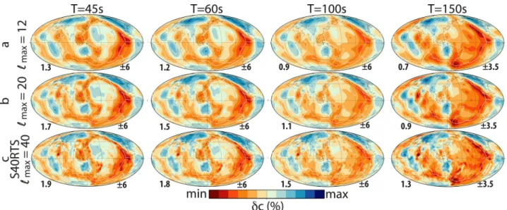
Figure 4.Rayleigh wave phase velocity maps calculated for mantle models withlmax=40 (S40RTS), 20 and 12 for wave periods∼45, 60, 100 and 150 s. These mantle models are combined with a homogeneous crustal layer and shall be referred as modelsa,bandcthroughout this paper. The numbers on the bottom left side of each map are roughness values (R×105_{, eq. 1). The numbers on the bottom right side of the maps represent the colour scale ranges} expressed in percentage with respect to the PREM model.

Figure 5.Power spectra of Rayleigh wave phase velocity maps atT∼100 s for the earth models considered in this study: (a) models obtained varyinglmax (Section 4.1.1); (b) models obtained varying the PV factor (Section 4.1.2); (c) models obtained varying the PO factor (Section 4.1.3); (d) models obtained by varying the crustal model (Section 4.2). Spectra are normalized with respect to the maximum value of each row of subplots.

Table 1. Roughness (Ras in eq. 1) values of all the Rayleigh wave phase velocity maps used in this study for wave periods ofT∼45, 60, 100 and 150 s. Roughness (×10−5) Models/Periods 45 s 60 s 100 s 150 s a lmax=12 1.3 1.2 0.9 0.7 b lmax=20 1.7 1.5 1.1 0.9 c lmax=40 1.9 1.8 1.5 1.3 d PV=0.5 1.0 0.9 0.7 0.5 e PV=1.0 2.0 1.9 1.3 0.9 f PV=1.75 3.5 3.3 2.3 1.6 g PO=1.5 2.9 2.8 2.0 1.7 h PO=2.0 3.9 3.7 2.6 1.8 i PO=3.0 5.9 5.5 3.9 2.7 j PO=3.5 6.8 6.4 4.6 3.2 k lmax=40 PO=3.0 5.7 5.4 4.5 3.9 l CRUST2.0 2.6 2.3 1.5 1.0 m const_moho 2.5 2.2 1.4 1.0

can be seen in Fig.5(b). Rayleigh wave phase velocity maps for S20RTS (PV = 1.0, PO = 1.0) are shown in Fig.6. Maps for PV=0.5 and PV=1.75 are not shown for brevity as they differ from those with PV=1.0 just by a constant factor.

The roughness of these models increases as the period decreases and PV increases. It ranges fromR=0.5×10−5_{for PV}₌_{0.5 and} T∼150 s toR=3.5×10−5_{for PV}₌_{1.75 and}_T_∼_{45 s (Table}₁_).

As these three models have the same smallest scale of hetero-geneity (lmax =20,∼2 000 km), considering the FRT validity

conditionλ, in theory we do not expect a strong dependency of the FRT’s performance on the PV factor.

4.1.3 Varying the strength of heterogeneity—PO factor

We build another subset of mantle models by varying the strength of the small-scale heterogeneity only. We apply a multiplicative factor (PO) to the spherical harmonic coefficients of S20RTS for

l larger or equal to 5. In other words, we increase the strength of heterogeneity with size smaller than about 7300 km, leaving those larger than 7300 km as in S20RTS. We use PO=1.0 (same as PV=1, S20RTS, modele), 1.5 (modelg), 2.0 (modelh), 3.0 (model

i) and 3.5 (modelj). Rayleigh wave phase velocity maps for these models are displayed in Fig.6and the power spectra are shown in Fig. 5(c). Finally, in order to obtain an end-member model with strong and rough heterogeneity, we also applied PO=3.0 to S40RTS (modelk).

Excluding the modelk, we do not increase the smallestof this subset of models (modelse,g,h,i,j). For this subset of modelsR

(6)

Figure 6.Rayleigh wave phase velocity maps calculated for mantle models with PO=1.0 (S20RTS), 1.5, 2.0, 3.0 and 3.5 for wave periodsT∼45, 60, 100 and 150 s. These mantle models are combined with a homogeneous crustal layer and shall be referred as modelse,g,h,iandj, respectively, throughout this paper. The numbers on the bottom left side of each map are roughness values (R×105, eq. 1). The numbers on the bottom right side of the maps represent the colour scale ranges expressed in percentage with respect to the PREM model.

increases as the period decreases and PO increases. It ranges from

R=0.9×10−5_{for PO}₌_{1.0 and}_T_∼_{150 s to}_R₌_6.8_×₁₀−5_for

PO=3.5 andT∼45 s (Table1).

It is worthy to illustrate the difference between the PV and PO factors. Fig.7shows examples of depth profiles at two locations when varying PV and PO. These profiles show that whereas the variations of the PV factor have a linear effect on the global strength of the perturbations, the PO factor can even change the sign of the anomalies in some cases (e.g. profile B, top, near 600 km of depth).

4.2 Crustal models

In addition to considering a homogeneous crust model (Moho depth = 24.4 km, Vs = 3.2 km s−1_, _Vp ₌ _{5.8 km s}−1_, _ρ ₌

2.6 g cm−3_{), we have also combined our set of mantle models with}

two 3-D crustal models.

We combine the mantle model S20RTS with the 3-D global crust model CRUST2.0 (modell). Moreover, in order to investigate the effects of variations in Moho depth, we also use a combination of the S20RTS mantle with a simplified version of CRUST2.0, where the Moho depth is maintained constant to 24.4 km (modelm). To build this model from CRUST2.0 we follow the same approach as in Parisiet al.(2015) whereby an increase (or decrease) of the Moho depth with respect to CRUST2.0 is compensated by an increase (or decrease) ofVs, applying the trade-off relationship between the Moho depth andVsreported by Lebedevet al.(2013).

Rayleigh wave phase velocity maps for S20RTS combined with these two 3-D crustal models are shown in Fig.8. Interestingly, the

effects of the crust are visible even forT∼150 s. Power spectra are shown in Fig.5(d) and the roughness values are summarized in Table1. While these two crustal models show different dispersion perturbations (Fig.8), the use of the trade-off relationship reported by Lebedevet al.(2013) helps ensure that the constant Moho model used is realistic and hence it is a useful model for our waveform comparisons.

5 R E S U L T S

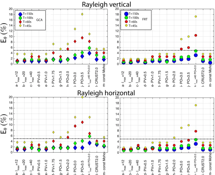
The results of the FRT–SEM and GCA–SEM waveform compar-isons are summarized in Figs9and10, where the medians of all the phase (Eφ) and amplitude (EA) errors are reported for each model

and each wave period. Following Parisiet al. (2015) and Dalton

et al.(2014), we prefer to use the median rather than the average to reduce the effects of outliers. Nevertheless, for completeness, we also present in the supplementary information two figures showing the percentage of measurements below the phase and amplitude thresholds considered (Supporting Information Figs S1 and S2). In the next subsections, we analyse the various factors affecting the performance of the FRT and GCA at predicting Rayleigh wave phase and amplitudes.

5.1 Effects of scale length of heterogeneity

Fig.9shows that increasinglmax(modelsa–c) only slightly affects Eφfor the FRT.Eφslightly increases with decreasing wave period, but, overall, for modelsa–cthe FRT accurately models Rayleigh wave phase, with E_φ being always below the 5 per cent error threshold for both vertical and horizontal component Rayleigh

(7)

Figure 7.Examples of depth profiles of shear velocity perturbations in the mantle showing the differences of varying the PO and PV factors.

Figure 8.Rayleigh wave phase velocity maps for wave periods∼45, 60, 100 and 150 s calculated for mantle model S20RTS combined with CRUST2.0 (top row) and a simplified version of CRUST2.0 with constant Moho depth (bottom row). These crustal models shall be referred as modelslandmthroughout this paper. The numbers on the bottom left side of each map are roughness values (R×105_{, eq. 1). The numbers on the bottom right side of the maps represent the} colour scale ranges expressed in percentage with respect to the PREM model.

waves. As for the GCA, the results are similar to the FRT, ex-cept that the phase errors forT∼45 s are larger, but still below the misfit threshold.

Regarding the amplitude errors, Fig.10 shows a clearer trend of increasing FRT errors withlmax. Nevertheless,EAare under or

at the error threshold of 10 per cent for modelsa–cfor vertical component Rayleigh waves and slightly above it for modelcfor horizontal component Rayleigh waves. On the other hand, GCA’s amplitude errors are always above the amplitude threshold except forT∼150 s vertical component Rayleigh waves, which are just below the misfit threshold in modelsa–c.

5.2 Effects of strength of heterogeneity 5.2.1 PV factor

Fig. 9for models d–fshows a good correlation between FRT’s

E_φand the PV factor for both vertical and horizontal component Rayleigh waves. Also, similar to the previous section,E_φ shows some anti-correlation with wave period and it never exceeds the phase misfit threshold. Similar to the previous case, GCA’s phase errors are somewhat larger than for the FRT, but they only exceed the misfit threshold forT∼45 s, for modelf.

(8)

Figure 9. Summary of the phase errorE_φatT∼60, 100 and 150 s for all the models used in this study for GCA (diamonds, left) and FRT (circles, right).E_φ

values are the medians for each model and period computed for all the paths illustrated in Fig.1. The horizontal black dash-dot lines correspond to the error thresholds of 5 per cent.

FRT’sEA for these models (modelsd–f; Fig.10) is overall

di-rectly correlated to the wave period. The threshold forEAis slightly

exceeded for the horizontal component of Rayleigh waves forT∼

150 s but the overall FRT performance in modelling Rayleigh wave amplitudes for this subset of models is good, whereas for the GCA the amplitude misfits always exceed the misfit threshold, except for

T∼150 s for modelsdande.

5.2.2 PO factor

Similar to the PV factor effect studied in the previous section, there is a good correlation between FRT’sE_φand the PO factor (models

e,g–j; Fig.9). The rate of increasing errors with PO is highest for

T∼45 s andT∼60 s. The overall FRT performance for this subset of models is good, except for the models iand jfor the shortest wave periods (T∼45 s andT∼60 s). The GCA’s phase misfits have a similar behaviour to the FRT, but they are always larger and exceed the misfit threshold for the shortest wave periods when PO

≥2 (modelsh,iandj).

The trend of FRT’sEA(Fig.10, modelse,g–j) against the period

for this subset of models is similar to that observed for the PV factor. The FRT performs poorly for models with PO=3.0 and 3.5 for all

periods considered, particularly for horizontal component Rayleigh wave amplitudes. The latter are also poorly modelled in the PO= 2.0 model forT∼150 s, being right at the threshold for all the other wave periods. Similar to the previous cases, the amplitude errors for the GCA are well above the misfit threshold in all cases, except forT∼150 s for PO≤2, where they are very close to the threshold. Figs9and10also show the results for the modelk, which is built by applying PO=3.5 to S40RTS. FRT and GCA phase and ampli-tude errors for this model are consistent with the results obtained when varyinglmaxand the PO factor. The amplitude modelling for

this model is poor for both the FRT and GCA and for all the wave periods considered. Moreover, the phase modelling is quite poor for the shortest wave periods considered (T∼60 s andT∼45 s).

5.3 Crustal effects

When comparing the effects of different crustal models, the FRT and GCA errors in phaseE_φ are slightly lower when using a ho-mogeneous crust, notably forT∼45 s. Nevertheless, FRT’sEφare below the phase misfit threshold in all cases for these three mod-els and the GCA’sE_φ only slightly exceed the threshold forT∼

45 s. On the other hand, FRT’sEA increases substantially when

(9)

Figure 10.Summary of the amplitude errorEAatT∼60, 100 and 150 s for all the models used in this study for GCA (diamonds, left) and FRT (circles, right).EAvalues are the medians for each model and period computed for all the paths illustrated in Fig.1. The horizontal black dash-dot lines correspond to the error thresholds of 10 per cent.

considering 3-D crustal effects (compare models e, l and m in Fig.10). However, the FRT amplitude modelling is still accurate for vertical component Rayleigh waves, except forT∼45 s.

5.4 Effects of the path length

The errors in phase and in amplitude for the FRT,E_φandEA, are

also analysed for different ranges of path lengths (Fig.11).E_φand

EAclearly increase with the epicentral distance at all periods

con-sidered.Eφis always under the phase misfit threshold (5 per cent) except forT ∼ 45 s and for T ∼ 150 s horizontal component Rayleigh waves, for distances larger than 110◦. On the other hand, the errors in amplitudeEAare under the amplitude misfit threshold

(10 per cent) for paths shorter than 110◦, with theT∼150 s am-plitude errors for horizontal component Rayleigh waves being very close or slightly above the misfit threshold for all distances.

The GCA (Supporting Information Fig. S3) shows similar trends ofE_φandEAas functions of epicentral distance, but the errors are

larger than for the FRT.Eφexceeds the misfit threshold forT∼45 s andT∼60 s for distances larger than about 100o_._E

A exceeds the

10 per cent threshold in all cases except forT∼150 s.

6 D I S C U S S I O N

6.1 Roughness to define the FRT validity domain

As explained previously, the goal of this study is to assess the domain of validity of the FRT when modelling long period surface waves in earth models that potentially can be either used or built during realistic waveform tomography experiments. In particular, we aim at obtaining quantitative criteria, which may provide guidance for future tomographic inversions.

The results presented in the previous section clearly highlight that the FRT is a highly accurate technique to model the phase of Rayleigh waves in almost all the models considered.E_φis, in fact, above the threshold of 5 per cent only for models with heterogeneity more than 3 times stronger than the heterogeneity of the S20RTS or S40RTS mantle models and mostly for periods shorter than 70–80 s (Fig.9).

The increase in FRT and GCA’s phase error with decreasing wave period is a common feature for all the models considered. This is an unexpected result because it does not follow the the-oretical validity expressed by λ . In particular, we observe that the shortest wave periods here considered, (T ∼ 45 s and

(10)

Figure 11. Phase (left) and amplitude (right) errors plotted as functions of epicentral distance, for models obtained by varying PV, PO andlmax. For each period, each point (circle) in the plot corresponds to the median of the errors for the models fromatojcalculated in bins of epicentral distance 20◦wide. The curves are obtained by linearly interpolating these bins.

T ∼60 s), are the most affected by the PO factor, that is, by the strength of small–scale heterogeneity. Due to the dispersion of sur-face waves, the shorter is the period, the shallower are the parts of the Earth sampled by the waves. In realistic earth models, the shal-lower parts of the mantle are those with the stronger anomalies and this increases wave scattering effects (especially due to small-scale anomalies affecting short period waves), which are not taken into account by the FRT and GCA. Inaccuracies in phase of Rayleigh waves can be controlled by considering paths shorter than 110◦. On the other hand, as expected, GCA’s phase errors are generally larger than for the FRT but they are below the misfit thresholds for the S20RTS and S40RTS models as well as for the smoother versions of these models considered. For PO≥1.5 the GCA breaks for the shortest wave periods considered. This suggests that future tomog-raphy studies based on phase information may benefit from using the FRT.

Conversely, the FRT’s accuracy of the amplitude modelling of Rayleigh waves mostly increases for the shorter periods except for

T ∼ 45 s for the most heterogeneous models (models i–m), re-specting the general ray theory validity conditionλ. In the framework of the FRT, the amplitude of the surface waves is a func-tion of the second derivative of the phase velocity map, calculated transversely to the ray (e.g. Ferreira & Woodhouse2007) within the Fresnel zone. For longer wave periods, the ray approximation is less accurate because it neglects the finite area of the Fresnel zone, whose width is proportional to the period. However, in more com-plex cases (e.g. in models with 3-D crust), we observe thatEAfor

vertical component Rayleigh waves decreases as the wave period

increases. The differences in behaviour between the vertical and hor-izontal components of Rayleigh waves when 3-D crusts are taken into account suggest that heterogeneity of the shallower parts of the models, as well as horizontal discontinuities, are the factors that mostly affect the accuracy of the modelling for the shortest periods. Moreover, horizontal component Rayleigh waves are more com-plicated to model in 3-D media than vertical components, because they are strongly affected, for example, by deviations in arrival angle from the great-circle path and also by coupling effects. Uncertain-ties related to coupling effects, which are not accounted in the FRT calculations, but are intrinsically included in the SEM modelling, may affect the horizontal components more strongly than the verti-cal component Rayleigh waves leading to the observed differences. Overall, our waveform comparisons indicate that FRT is accurate at calculating even the amplitude of Rayleigh waves as long as models with PO and PV factors larger than 3.0 and periods longer than 150 s or shorter than 45 s are avoided. These inaccuracies in modelling the amplitude of Rayleigh waves can be controlled by considering paths shorter than 110◦. Moreover, it should be noted that the mod-els with PO and PV factors≥3 lead to seismic velocity anomalies of∼20 per cent, which may not be realistic. Finally, we found that apart from the longest wave periods considered (T∼150 s), the GCA is unable to accurately model Rayleigh wave amplitudes.

As seen in Section 4.1.1, we expected the FRT to break down for modelscandk(lmax=40), especially at longer periods, where

the wavelength is almost comparable to the smallest scale length of heterogeneity of these two models. Nevertheless, the FRT performs well for modelc(S40RTS), except forT ∼150 s for horizontal

(11)

Figure 12.Scatter plot ofEφandEAagainst the roughnessR(eq. 1) of the corresponding phase velocity map. The different symbols correspond to distinct families of models: (i) varyinglmax(modelsa–c; squares); (ii) varying the PV factor (modelsd–f; triangles); (iii) varying the PO factor (modelsg–j; diamonds); (iv) varying bothlmaxand PO factor (modelk); (v) with 3-D crustal structure (modelsl–m; stars).

component Rayleigh waves. On the other hand, the FRT breaks down in model k because of the large PO factor applied (3.0), which suggests that the overall roughness of the models controls the validity of the FRT rather thanlmaxalone.

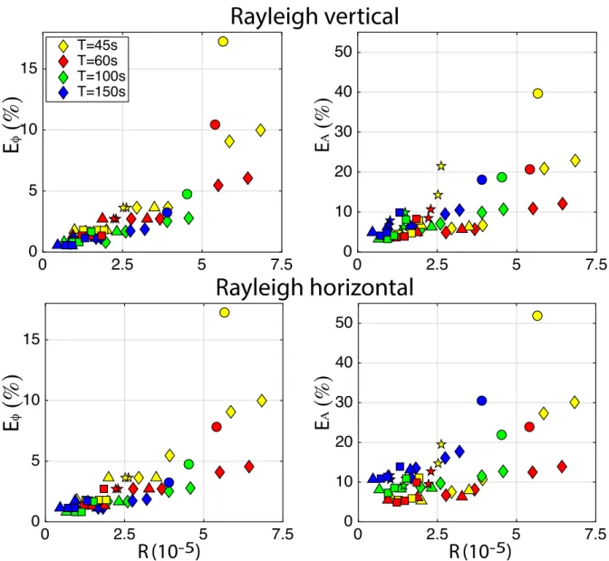
To generalize the outcome of our FRT-SEM waveform compar-ison experiment, in Fig.12we have plottedE_φandEAagainst the

model roughnessR(eq. 1; see Table1for a summary ofRfor all the models considered in this study).E_φis related toRwith a cor-relation coefficient of 0.89 for the vertical component and 0.84 for the horizontal component. The plot highlights that FRT is a valid approximation to calculate the phase of Rayleigh waves whenRof the phase velocity map is less than about 5.0×10−5_.

The correlations are stronger with different wave periods are considered separately (0.72, 0.72, 0.77 and 0.77 for the wave periods of∼45, 60, 100 and 150 s). The scatter plot suggests that FRT is a good approximation to model the amplitude of vertical component Rayleigh waves in the range of periods considered whenR<4.0

×10−5_{. Similar thresholds can be used for horizontal component}

Rayleigh waves, except forT∼150 s, for whichR<1.25×10−5

seems more appropriate.

6.2 Comparisons with real data

This study is based on the analysis of Rayleigh wave phase and amplitude forward modelling errors, using as thresholds of misfit goodness 5 and 10 per cent for phase and amplitudes, respectively. In order to better interpret the meaning of the modelling errors studied, in this section we show illustrative comparisons between real data and FRT, GCA and SEM predictions.

We have computed phase and amplitude errors as in Section 3.1 but since the comparison is performed between the three types of theoretical seismograms and the data, we refer to these errors as phase and amplitude misfits (δφandδA, respectively).

All the three earthquakes shown in Fig.1are considered and we use the mantle model S20RTS combined with the crustal model CRUST2.0 (modell) for the computations. Due to the limited qual-ity of horizontal component real data, we only present results for vertical component Rayleigh waves. Fig. 13 shows scatter plots between FRT (blue)/GCA (red) data misfits and SEM data misfits.

Overall, compared to the GCA misfits, the FRT misfits (δφ and δA) are always closer to the SEM misfits, with correlation

(12)

Figure 13. Scatter plots between the data misfits (δφ, top andδA, bottom) calculated for FRT (blue circles) and GCA (red circles) against the data misfit calculated for SEM for each wave period considered. Numbers within the plot are the correlation coefficients for GCA and FRT data misfits against SEM data misfits.

coefficients larger than 0.67 in all cases. The GCA and FRTδφare similar, with small differences in the correlation coefficients, except for the wave period of∼45 s where the correlation coefficients are 0.72 for GCA and 0.93 for FRT. This result is consistent with the

E_φshown in Fig.9confirming that the FRT is more accurate than the GCA, especially when modelling short period surface waves.

As expected, while the FRT amplitude misfits are quite similar to SEM in all cases, the GCA amplitude anomalies show little correlation with SEM, especially for long wave periods (T∼100 s andT∼150 s) where the correlation coefficients are small (0.55 and 0.23, respectively). These results highlight the poor ability of GCA at predicting Rayleigh wave amplitudes.

Moreover, the range of observed real data misfits is much larger than in the synthetic tests carried out in this study (Supporting Information Table S1). This provides us not only an additional con-firmation that the chosen misfit thresholds are reasonable, but also further confirms that the errors associated with the FRT approach are much smaller than observed differences between real data and theoretical predictions for current existing 3-D Earth models.

6.3 Comparison with previous studies 6.3.1 GCA versus FRT

A few studies have showed the larger accuracy of the FRT with respect to the GCA, especially when modelling surface wave am-plitudes. Early studies (Wang & Dahlen1994; Larsonet al.1998) achieved this result by direct comparison of the FRT and GCA pre-dictions. Wang & Dahlen (1994) compared the amplitude predic-tions for the FRT—with and without the local source and receiver excitations taken into account (in this work local excitations are taken into account)—and they found that the differences in the wave amplitude were around 30 per cent. These were even larger between

the complete FRT and the GCA. Larsonet al.(1998) compared FRT and GCA predictions and concluded that while for the phase modelling the GCA could be adequate, the amplitude modelling needed the more sophisticated calculations of the FRT.

More recent works used accurate numerical methods as ground truth to compare the FRT and GCA accuracies. Romanowiczet al.

(2008) applied the nonlinear asymptotic mode coupling theory (Li & Romanowicz1995) taking into account off great-circle effects. They found that, in most of the cases, the waveform errors (a com-bination of the phase and amplitude errors) decrease when the exact ray-tracing was used. Peteret al.(2009) used a simplified mem-brane approach and highlighted that the improvement of the phase anomalies predictions of the FRT over the GCA increases with the number of the surface wave orbits.

Daltonet al.(2014) focused on the amplitude predictions only and found that the errors of the GCA were systematically larger than the errors of the FRT. Our study confirmed the larger accu-racy of the FRT with respect to the GCA in the context of current tomographic models, especially when modelling surface wave am-plitudes. We find that while the GCA is valid to model the phase of Rayleigh waves for current existing Earth models such as S20RTS and S40RTS, it breaks for more heterogeneous models and partic-ularly for the shortest wave periods considered (T∼45 s andT∼

60 s). On the other hand, the GCA only predicts surface wave am-plitudes accurately forT∼150 s for current tomographic models.

6.3.2 Validity domain of the FRT

The domain of validity of the FRT was investigated in a few previous studies. Wang & Dahlen (1995) tested the FRT for three earth models and found thatδcand∇∇δcare good proxies for the errors in phase and amplitude, respectively, but general values of guidance were not given. A remarkable difference with our study is that

(13)

the earth models used by Wang & Dahlen (1995) did not have crustal structure and consisted of only three mantle models with differentlmax(from 12 to 36). In addition, ground truth synthetics

were calculated using a normal mode coupling technique, which involves some theoretical approximations (Um & Dahlen1992).

Other studies (e.g. Kennett & Nolet1990; Lebedevet al.2005; Schaeffer & Lebedev2013) attempted to define the validity bounds of their modelling of the phase of Rayleigh waves when consider-ing a sensitivity area around the ray. The correspondconsider-ing domain of validity was defined by analysing the trade-off between wave fre-quency and epicentral distance (Schaeffer & Lebedev2013). Similar to our study, these authors also found a decrease in the accuracy of the phase modelling with decreasing wave period for the epicentral distances considered in our work. This is probably due to enhanced scattering effects with decreased wave periods.

The trends of amplitude errors of Rayleigh waves are in line with the results of Daltonet al.(2014). The authors used two different earth models differing by a factor similar to our PO factor, but forlmax >18, to test the FRT against other amplitude modelling

techniques. As in this paper, they found an increase of the error in amplitude with increasing PO factor, wave period and epicentral distance, but in this study we consider a larger set of models and achieve more general conclusions.

7 C O N C L U S I O N S

We have assessed the accuracy of the surface wave FRT when modelling the phase and amplitudes of relatively long period surface waves (T∼45–150 s), using the SEM as ground truth.

We have found that the FRT is accurate in modelling the phase and the amplitude of Rayleigh waves for all the models considered, except for the three roughest models that exhibit anomalies up to 20 per cent. In the range of wave period studied, the accuracy when modelling Rayleigh wave phase decreases as the period decreases. This is probably due to strong small-scale heterogeneities sampled by the shorter period waves, resulting in strong scattering effects. We also found that the GCA does not predict Rayleigh wave amplitudes well, notably for the shortest wave periods considered (T∼45 s andT∼60 s). In addition, although the GCA accurately predicts Rayleigh wave phase for current earth models such as S20RTS and S40RTS, the phase errors of the FRT are smaller, particularly for the models with PV=1.75, PO=1.5 and PO=2.0. This suggests that the FRT is a useful technique to build new models of both elastic and anelastic structure.

This study shows that model roughness, expressed as the gradient of the phase velocity maps, is a good indicator of the accuracy of the FRT. Our results suggest that FRT is a good approximation for predicting the phase of Rayleigh waveforms when the average roughness ofδc(θ,) is less than 5.0 ×10−5_{. The accuracy of}

the amplitude modelling depends on the wave period considered and is poorer for horizontal component Rayleigh waves than for vertical components. We predict a good amplitude modelling of the vertical component Rayleigh wave for models withR<4.0× 10−5_{. If rougher earth models are used to simulate the amplitude of}

Rayleigh waves with the FRT, paths shorter than 100◦–110◦should be considered.

Our results show that there is scope to build future improved global tomographic models based on the FRT. The domain of va-lidity defined in this study can serve as a useful guide in future seismic tomographic inversions using the FRT as a forward mod-elling scheme.

A C K N O W L E D G E M E N T S

We sincerely thank Eric Debayle, an anonymous reviewer and the editor Andrea Morelli for their detailed reviews, which helped im-prove our manuscript. This research was carried out on the High Performance Computing Cluster supported by the Research and Specialist Computing Support services at the University of East Anglia and on Archer, the UK’s National Supercomputing Ser-vice. Some figures were built using Generic Mapping Tools (GMT; Wessel & Smith 1998). This work was supported by the Euro-pean Commission’s Initial Training Network project QUEST (con-tract FP7-PEOPLE-ITN-2008-238007, http://www.quest-itn.org) and the University of East Anglia. The Incorporated Research Insti-tutions for Seismology (IRIS) was used to access the waveform data from the IRIS/IDA network II (http://dx.doi.org/doi:10.7914/SN/II) and IU (http://dx.doi.org/doi:10.7914/SN/IU). AMGF also thanks funding by the Fundacao para a Ciencia e Tecnologia (FCT) project AQUAREL (PTDC/CTE-GIX/116819/2010).

R E F E R E N C E S

Anderson, D.L., Schreiber, E., Liebermann, R.C. & Soga, N., 1968. Some elastic constant data on minerals relevant to geophysics,Rev. Geophys., 6,491–524.

Auer, L., Boschi, L., Becker, T.W., Nissen-Meyer, T. & Giardini, D., 2014. Savani: a variable resolution whole-mantle model of anisotropic shear velocity variations based on multiple data sets,J. geophys. Res.,119(4), 3006–3034.

Bassin, C., Laske, G. & Masters, G., 2000. The current limits of resolution for surface wave tomography in North America,EOS, Trans. Am. geophys. Un.,81,F897.

Bozdag, E., Lefebvre, M., Peter, D., Smith, J., Komatitsch, D. & Tromp, J., 2015. Plumes, hotspots and slabs imaged by global adjoint tomography,

AGU Fall Meeting Abstracts S13C-06, AGU, San Francisco, CA. Chang, S.-J., Ferreira, A.M.G., Ritsema, J., van Heijst, H.J. & Woodhouse,

J.H., 2015. Joint inversion for global isotropic and radially anisotropic mantle structure including crustal thickness perturbations,J. geophys. Res.,120(6), 4278–4300.

Dalton, C.A., Hjörleifsdóttir, V. & Ekström, G., 2014. A comparison of approaches to the prediction of surface wave amplitude,Geophys. J. Int., 196,386–404.

Debayle, E. & Ricard, Y., 2012. A global shear velocity model of the upper mantle from fundamental and higher Rayleigh mode measurements,J. geophys. Res.,117(10), doi:10.1029/2012JB009288.

Dziewo´nski, A.M. & Anderson, D.L., 1981. Preliminary reference Earth model,Phys. Earth planet. Inter.,25(4), 297–356.

Ferreira, A.M.G. & Woodhouse, J.H., 2007. Source, path and receiver effects on seismic surface waves,Geophys. J. Int.,168(1), 109–132.

French, S.W. & Romanowicz, B.A., 2014. Whole-mantle radially anisotropic shear velocity structure from spectral-element waveform tomography,

Geophys. J. Int.,199(3), 1303–1327.

Kennett, B.L.N. & Nolet, G., 1990. The interaction of the S-wavefield with upper mantle heterogeneity,Geophys. J. Int.,101(3), 751–762. Komatitsch, D., Erlebacher, G., G¨oddeke, D. & Mich´ea, D., 2010.

High-order finite-element seismic wave propagation modeling with MPI on a large GPU cluster,J. Comput. Phys.,229(20), 7692–7714.

Komatitsch, D. & Tromp, J., 2002a. Spectral-element simulations of global seismic wave propagation—I. Validation,Geophys. J. Int.,149(2), 390– 412.

Komatitsch, D. & Tromp, J., 2002b. Spectral-element simulations of global seismic wave propagation—II. Three-dimensional models, oceans, rota-tion and self-gravitarota-tion,Geophys. J. Int.,150(1), 303–318.

Komatitsch, D. & Vilotte, J.-P., 1998. The spectral element method: An efficient tool to simulate the seismic response of 2D and 3D geological structures,Bull. seism. Soc. Am.,88(2), 368–392.

(14)

Larson, E.W.F., Tromp, J. & Ekstr¨om, G., 1998. Effects of slight anisotropy on surface waves,Geophys. J. Int.,132(3), 654–666.

Lebedev, S., Adam, J.M.-C. & Meier, T., 2013. Mapping the Moho with seismic surface waves: a review, resolution analysis, and recommended inversion strategies,Tectonophysics,609,377–394.

Lebedev, S., Nolet, G., Meier, T. & van der Hilst, R.D., 2005. Automated multimode inversion of surface and S waveforms,Geophys. J. Int.,162(3), 951–964.

Li, X.-D. & Romanowicz, B., 1995. Comparison of global waveform inver-sions with and without considering cross-branch modal coupling, Geo-phys. J. Int.,121(3), 695–709.

Moulik, P. & Ekstr¨om, G., 2014. An anisotropic shear velocity model of the Earth’s mantle using normal modes, body waves, surface waves and long-period waveforms,Geophys. J. Int.,199(3), 1713–1738.

Panning, M.P., Capdeville, Y. & Romanowicz, B.A., 2009. Seismic wave-form modelling in a 3-D Earth using the Born approximation: Potential shortcomings and a remedy,Geophys. J. Int.,177(1), 161–178. Parisi, L., Ferreira, A.M.G. & Capdeville, Y., 2015. Validity domain of

the Born approximation for seismic waveform modelling in realistic 3-D Earth structure,Geophys. J. Int.,200,908–914.

Peter, D., Boschi, L. & Woodhouse, J.H., 2009. Tomographic resolution of ray and finite-frequency methods: a membrane-wave investigation,

Geophys. J. Int.,177(2), 624–638.

Ritsema, J., Deuss, A., Van Heijst, H.J. & Woodhouse, J.H., 2011. S40RTS: A degree-40 shear-velocity model for the mantle from new Rayleigh wave dispersion, teleseismic traveltime and normal-mode splitting func-tion measurements,Geophys. J. Int.,184(3), 1223–1236.

Ritsema, J., Van Heijst, H.J. & Woodhouse, J.H., 1999. Complex shear wave velocity structure imaged beneath Africa and Iceland,Science,286(5446), 1925–1931.

Robertson, G.S. & Woodhouse, J.H., 1995. Evidence for proportionality of P and S heterogeneity in the lower mantle,Geophys. J. Int.,123(1), 85–116. Romanowicz, B., 1987. Multiplet-multiplet coupling due to lateral hetero-geneity: asymptotic effects on the amplitude and frequency of the Earth’s normal modes,Geophys. J. R. astr. Soc.,90(1), 75–100.

Romanowicz, B.A., Panning, M.P., Gung, Y. & Capdeville, Y., 2008. On the computation of long period seismograms in a 3-D earth using normal mode based approximations,Geophys. J. Int.,175(2), 520–536. Schaeffer, A.J. & Lebedev, S., 2013. Global shear speed structure of the

upper mantle and transition zone,Geophys. J. Int.,194(1), 417–449. Tromp, J. & Dahlen, F.A., 1992a. Variational principles for surface wave

propagation on a laterally heterogeneous earth—I. Time-domain JWKB theory,Geophys. J. Int.,109,581–598.

Tromp, J. & Dahlen, F.A., 1992b. Variational principles for surface wave propagation on a laterally heterogeneous Earth—II. Frequency-domain JWKB theory,Geophys. J. Int.,109(3), 599–619.

Um, J. & Dahlen, F.A., 1992. Normal mode multiplet coupling on an as-pherical, anelastic earth,Geophys. J. Int.,111(1), 11–31.

Wang, Z. & Dahlen, F.A., 1994. JWKB surface-wave seismograms on a laterally heterogeneous earth,Geophys. J. Int.,119,381–401.

Wang, Z. & Dahlen, F.A., 1995. Validity of surface-wave ray theory on a laterally heterogeneous earth,Geophys. J. Int.,123,757–773.

Wessel, P. & Smith, W.H.F., 1998. New, improved version of the Generic Mapping Tools released, EOS, Trans. Am. geophys. Un., 79,579.

Woodhouse, J.H., 1974. Surface waves in a laterally varying layered struc-ture,Geophys. J. R. astr. Soc.,37(2), 461–490.

Woodhouse, J.H. & Dziewo´nski, A.M., 1984. Mapping the upper mantle: three-dimensional modeling of Earth structure by inversion of seismic waveforms,J. geophys. Res.,89(B7), 5953–5986.

Woodhouse, J.H. & Wong, Y.K., 1986. Amplitude, phase and path anomalies of mantle waves,Geophys. J. R. astr. Soc.,87,753–773.

S U P P O RT I N G I N F O R M AT I O N

Additional Supporting Information may be found in the online ver-sion of this paper:

Figure S1.Percentage of all FRT (circles) and GCA (diamonds) waveforms withE_φless than 5 per cent for each model and wave period considered.

Figure S2.Percentage of all FRT (circles) and GCA (diamonds) waveforms withEAless than 10 per cent for each model and wave

period considered.

Figure S3. Phase (left) and amplitude (right) errors for GCA wave-forms plotted as functions of epicentral distance, for models ob-tained by varying PV, PO andlmax. For each period, each point

(circle) in the plot corresponds to the median of the errors for the models fromatojcalculated in bins of epicentral distance 20◦wide. The curves are obtained interpolating the obtained points.

Table S1.Middle column: data misfits in phase (δφ) and amplitude (δA) for synthetic waveforms calculated with GCA, FRT and SEM. Right column: errors in phase (Eφ) and amplitude (EA) for

wave-forms calculated with GCA and FRT (against SEM). Misfits and errors are shown at wave period ofT∼45, 60, 100 and 150 s. (http://gji.oxfordjournals.org/lookup/suppl/doi:10.1093/gji/ ggw005/-/DC1)

Please note: Oxford University Press is not responsible for the con-tent or functionality of any supporting materials supplied by the authors. Any queries (other than missing material) should be di-rected to the corresponding author for the paper.