Development of Software Effort Estimation using a Non Fuzzy Model

(1)

Development of Software Effort Estimation using a Non Fuzzy

Model

H P Patra, Kumar Rajnish

Department of Computer Science, BIT Mesra, Ranchi, India

E-mail: [email protected], [email protected]

Abstract

Now day’s accurate estimation of the software effort is a challenging issue for the modern software developers. So, to bind a contract depends purely on the estimated cost of the software. Over estimate or under estimate lead a loss or gain of the software project and also increase the probability of success and failure of the project and delay of delivery date. In this paper, we use a non fuzzy conditional algorithm to build a suitable model structure to use the improved estimation for NASA software projects. We plan to set of linear conditional models using the domain of possible KLOC (Kilo Lines of Code). The performance of developed model was analyzed using NASA data set and we compare with the result of COCOMO tuned-PSO, Halstead, Walston -Felix, Bailey-Basili and Doty models were provided.

Keywords: Lines of code, software cost estimation, MRE, MMRE, PRED

Abbreviation

KLOC : Kilo Lines of code MRE :Magnitude of relative error MMRE :Mean Magnitude of relative error PRED : Prediction

NLOC : New Lines of Code TLOC : Total Lines of code DLOC : Developed Lines of Code ME : Methodology

FP : Function points MM : Man-Months

CC :Cumulative complexity INTRODUCTION

This paper focused to satisfy the need of today’s software industry by estimating the cost and effort and challenging the various issues and variations occurred in software size. Accuracy and timely estimation of software efforts is one of the most critical activities to manage a software project. As both over estimate and under estimate of software is very harmful for modern software industry this paper gives emphasis to predict the effort accurately and reliably. If the estimation is low then the software development team will be under pressure to finish the product and if

the estimation is high then the most of the resources will be commuted to the project. Accurate estimate Implies better planning and efficient use of resources such as cost, duration and effort for space and military projects[1–3]. Previously, estimation was done by human experts, but in the recent era estimation is carried out using so many computer-based learning techniques [4, 5]. In 1995, Standish Pvt Ltd analyzed over 8000 projects to estimate the budget and found that 90% are overestimated and 50% of completed project cannot fulfill the original requirements and 10% of projects are

(2)

prevent this problem so many estimation models are presented in presented [7–12]. In this paper, we compare the newly developed model with fuzzy COCOMO model [13–20]. The author describes about Genetic Algorithms for effort estimation. In this paper, we are analyzing an idea of using non-parametric Computing Techniques to build a new model with better accuracy to estimate the effort.

BASIC SOFTWARE PROJECT

ESTIMATION TECHNIQUES

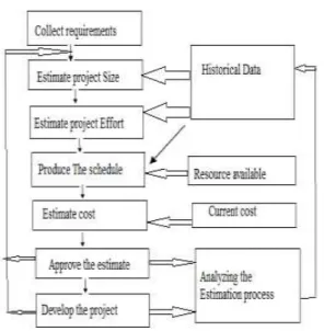
Software Effort estimation has been computed normally using parametric models considering the size of the size of the software project, which are the KLOC or function points. The steps summarized for basic software estimation is as follows:

1. Estimate the size metric of the software project, i.e., KLOC or Function Points (FP).

2. Estimate the effort in man-months, i.e., MM

3. Estimate the schedule in months (days).

4) Estimate the project cost using p effort and schedule.

The traditional software estimation procedure was described and shown in Figure 1.

Fig. 1: Traditional Software Estimation Procedure.

SIZE ESTIMATION

There are two main methods can be used to estimate software size, i.e., Estimation by analogy and Estimation by product size Estimation by analogy is carried out by an experienced estimator considering the project size of available previous project and focusing the similarity of the new one. Estimation by product size is carried out using the product features and using the algorithmic approach such as FP.

ESTIMATION OF EFFORT

There are so many model are developed for software project effort estimation. Some of the models for software effort estimation are given in Table1. These models have been derived analyzing huge number of completed projects of different organization.

(3)

These models give different results considering the type of software projects [8].

SCHEDULE ESTIMATION

From the effort estimation the schedule can also be estimated considering the no of people required to perform the task. In this phase the following factors should be considered, i.e., who will work on the project, what they will do, when project starts and when project finish.

COST ESTIMATION

To estimate the total cost one should consider the factors like labor cost, hardware and software purchases or rentals, travel for meeting or testing purposes, training the developers, Telecommunications, office space, and so on. Thus Cost of project is $ (Effort * Monthly Wages) * Total months.

COCOMO MODEL

A project manager of the company has the responsibility to identify the cost of the software to evaluate the project progress against the specified budget and schedule. As the main cost driver for software development is the effort. The basic element that affects the effort estimation is, the developed kilo line of code (KLOC) which includes the program instructions and statements [9]. The COCOMO is the basic parametric model used to estimate software which was researched and developed by Boehm at TRW. Here, Mrs. Boehm grouped the projects into three different software domains, organic, semidetached and embedded. COCOMO

model was developed considering the linear equation comes in the form given in Equation as shown in equation 1.

Effort =a (KLOC)b ………… (1)

Where the effort is computed in PM (person-months) and the parameter a, b depends on the type of software, i.e., Organic, Semi-Detached or Embedded.

EFFORT ESTIMATION MODEL

USED IN THIS STUDY

As we know Effort=f (KLOC, ME)

Where KLOC is the kilo lines of code and ME is the methodology used in the software and f () is a nonlinear function in terms of LOC and ME. We present three different functions for f () to compute the effort expressed as below.

M1. Effort=5.25×101×KLOC+5.28×101+Log(ME)×10 where KLOC>=50

M2. Effort=2.02*100*KLOC-5.62*Log(ME) Where 10>=KLOC<50

M3. Effort=7.92*101*KLOC+3.18*Log(ME) Where KLOC<10

This modeling study is based on the statistical analysis of the effort in following dataset given below Table 2. It has the following six effort drivers or project attributes:

 Total lines of code (TLOC),  New lines of code (NLOC),

 Developed lines of code (DLOC) (all three in KLOC),

 Total methodology (TME),  Cumulative complexity (CC) and  Cumulative experience (CE).

The following solution may be used to find the optimal values of the model parameters. Minimize ( 2 1( _ _ )



  n

i E actual E computed where

E_actual is the actual effort and E_computed is the measured Effort. Optimization algorithm has applied on the following data which consist of two independent variable KLOC and ME and One dependent variable Effort.

(4)

DATA COLLECTION

We are collecting the data from the data set presented by Bailey and Basili which consists of two variable KLOC in Kilo Lines of Code and Effort in Man–Month [1]. The detail data set is given in Table 2 in which 13 projects are taken as training case and 5 are for testing and validating the model. Table 2 Pr. (KLOC) No Developed Actual ME CC Lines Effort 1 90.2 115.8 30 21 2 46.2 96 20 21 3 46.5 79 19 21 4 54.5 90.8 20 29 5 31.1 39.6 35 21 6 67.5 98.4 29 29 7 12.8 18.9 26 25 8 10.5 10.3 34 19 9 21.5 28.5 31 27 10 3.1 7 26 18 11 4.2 9 19 23 12 7.8 7.3 31 18 13 2.1 5 28 19 14 5 8.4 29 21 15 78.6 98.7 35 33 16 9.7 15.6 27 21 17 12.5 23.9 27 33 18 100.8 138.3 34 33 PERFORMANCE OF THE PROPOSED MODEL

Table 3 shows the result of effort estimation by the proposed model as comparison to other models and Table 4 shows the effort variance of proposed model in accordance with the data of 18 given projects and measure the performance to validate the outcome. Table 5 shows the MMRE and RMSE of different models as comparison with proposed model.

EVALUATION CRITERIA AND

ERROR ANALYSIS

There are so many statistical approaches are used to estimate the accuracy of the software effort. We are using methods like MRE, MMRE, RMSE, and Prediction. Boehm suggested a formula to find out the error percentage as shown below [2]:

Error%= *100 _ _ _ Pr Effort Actual Effort Actual Effort edicted  _..(2) MRE (Magnitude of Relative Error): We can calculate the degree of estimation error for individual project.

MRE= ) 3 ...( _ | _ Pr _ | Effort Actual Effort edicted Effort Actual 

RMSE (Root Mean Square Error): We can calculate it as the square root of the mean square error and can be defined as. RMSE= ) 4 ...( 1 2 ) _ Pr _ ( 1  n 

i Actual Effort edicted Effort n

MMRE (Mean Magnitude of Relative Error): It is another way to measure the performance and it calculates the percentage of absolute values of relative errors. It is defined as.

MMRE=  n  i _Actual _Effort Effort Actual effort edicted n 1 _ ...(5) | _ _ Pr | 1

PRED (N) This criteria is used to calculate the average percentage of estimates that were within N% of the actual values, i.e., the percentage of predictions that fall within p % of the actual, denoted as PRED (p).Where k is the number of projects in which MRE is less than or equal to p, and n is the total number of projects. It is defined as

PRED (p) = k / n

Variance Absolute Relative Error (VARE). VARE criteria in order to percent of variance to estimate the value of each project can be calculated

(5)

For project1 having KLOC =90.2 the actual effort is 115.8 Man-Month and the calculated effort for PSO based COCOMO is 128.43 by the proposed model is 114.92 MM. Similarly for project 2 KLOC=46.2 the actual effort is 96 MM and calculated effort for PSO based COCOMO is 71.37 and by the proposed model is 86.01 MM. Now we can calculate the % of error using the equation 5. For project 1, the error % for PSO based COCOMO is (10.90) % and error % for proposed model is (-0.075) %. Similarly for project 2, the error % for PSO based COCOMO is (-25%) % and error % for proposed model is (-10.4) %. Here the negative % indicates the under estimation of the project and positive % error indicates the project is over estimate. Big under estimate gives extra pressure to the developing staff and leads to add more staffs which causes the late to finish the project. According to Parkinson’s Law “Work expands to fill the time available for its completion” Big over estimation reduces the productivity of personnel’s [15]. So during estimation the researchers should have to give emphasis to reduce the big over or under estimation of the project. Performance of different models are shown in Table5 and Effort variance (%) by proposed Model (NASA data) is shown in Table 4 [1].

Table4: (Effort Variance of proposed Model).

Project Actual Proposed Effort No KLOC Effort Effort Variance % _____________________________ 1 90.2 115.8 114.92 0.75 2 46.2 96 86.01 0.10 3 46.5 79 86.74 0.097 4 54.5 90.8 94.42 0.039 5 31.1 39.6 54.14 0.367 6 67.5 98.4 102.86 0.045 7 12.8 18.9 17.90 0.052 8 10.5 10.3 12.60 0.223 9 21.5 28.5 35.04 0.229 10 3.1 7 6.95 0.71 11 4.2 9 7.39 0.178 12 7.8 7.3 10.92 0.495 13 2.1 5 6.26 0.252 14 5 8.4 8.61 0.025 15 78 98.7 109.19 0.106 16 9.7 15.6 12.23 0.216 17 12.5 23.9 17.20 0.280 18 100.8 138.3 121.03 0.124 Table 5: Perfo rman ce Halst ead PSO _ COC OM O Propo sed Wals ton-Felix Bail ey-Bas il Doty MM RE 0.14 79 0.00 74 0.002 3 0.08 22 0.0 095 0.18 48 RMS E 215. 91 9.32 1 6.837 96.6 5 12. 31 233. 48 G-1 0 50 100 150 200 250 MMRE RMSE

The result of PSO Based COCOMO model effort estimation are taken from and the analysis has been carried out by using PSO Optimization Tool box developed in MATLAB to produce both for training and testing cases. We describe the result for given projects using different models like Halstead, Walston-Felix and others for comparison.

ADVANTAGES OF PROPOSED

MODEL  It Is reusable

(6)

 It calculates software development effort as a function of program size expressed in Kilo Lines of code (KLOC) and the methodology used to develop the project.

 It predicts the estimated effort with more accuracy.

 Researchers may further change the parameters to predict the better result.

G2 0 20 40 60 80 100 120 140 160 180 200 P1 P3 P5 P7 P9 P11 P13 P15 P17 E ff o rt

Proposed Vs Actual Effort

Proposed Actual Effort

Computed Effort for NASA Software Projects of different models as shown in Table 3 Table 3

Project Actual PSO Based Walston Bailey Halstead Doty Proposed No. KLOC Effort COCOMO Felix Basil Model Model Model __________________________________________________________________________ 1 90.2 115.8 128.43 312.78 140.8 599.66 589.37 114.92 2 46.2 96 71.37 170.14 67.77 219.81 292.53 86.01 3 46.5 79 71.78 171.15 68.24 221.96 294.51 86.74 4 54.5 90.8 82.51 197.75 80.92 181.63 347.77 94.42 5 31.1 39.6 50.42 118.69 44.84 121.4 199.29 54.14 6 67.5 98.4 99.57 240.25 102.1 388.19 435.08 102.86 7 12.8 18.9 23.12 52.91 19.55 32.05 76.3 17.90 8 10.5 10.3 19.43 44.18 16.66 23.81 62.01 12.60 9 21.5 28.5 36.46 84.82 31.14 69.78 131.32 35.04 10 3.1 7 6.6 14.55 8.21 3.82 17.28 6.95 11 4.2 9 8.6 19.19 9.35 6.02 23.75 7.39 12 7.8 7.3 14.96 33.71 13.40 15.24 45.42 10.92 13 2.1 5 4.7 10.21 7.22 2.13 11.49 6.26 14 5 8.4 10.12 22.49 10.22 7.82 28.51 8.61 15 78.6 98.7 113.8 275.95 120.8 487.7 510.26 109.19

(7)

16 9.7 15.6 18.12 41.11 15.68 21.14 57.07 12.23

17 12.5 23.9 22.64 51.78 19.16 30.93 74.43 17.20

18 100.8 138.3 141.59 346.06 159.4 708.41 662.08 121.03

Effort Estimation Graph of Different Models as shown in G-3 G-3 0 100 200 300 400 500 600 700 800 P1 P2 P3 P4 P5 P6 P7 P8 P9 P10 P11 P12 P13 P14 P15 P16 P17 P18

Actual Effort PSO COCOMO Halstead Walston-Felix

Bailey-Basili Doty Proposed

CONCLUSION AND FUTURE WORK This proposed model can be useful to estimate the software effort with better accuracy which is very important when software pays a lot in every industry. The predicted result shows there is very close values between actual and estimated effort. The effort variance is very less and the proposed model has the lowest MMRE and RMSSE. So, the proposed model may able to provide good estimation capabilities for today’s software industry. In future we plan to explore use of Rule based Fuzzy logic and Generic programming (GP) to build suitable model

for software estimation. REFERENCES

1. Bailey, J. W. and Basili , V. R. “A meta model for software development

resource expenditure,” in Proceedings of the International Conference on Software Engineering, (1981.) pp. 107–115.

2. Briand, L. C, Emam, K. E. and Wieczorek , I. ,“Explaining the cost of European space and military projects,” in ICSE ’99: Proceedings of the 21st international conference on Software engineering, (Los Alamitos, CA, USA), IEEE Computer Society Press, (1999). pp. 303–312.

3. Park R, J. W., Goethert, W , “Software cost and schedule estimating: A process improvement initiative,” tech. rep., (1994).

4. Shepper M. and Schofield, C. “Estimating software project effort using analogies,” IEEE Tran. Software

(8)

743

5. Group, T. S, CHAOS Chronicles. PhD thesis, Standish Group Internet Report, (1995).

6. Boraso, M. Montangero, C. and Sedehi, H. “Software cost estimation: An experimental study of model performances,” tech. rep., (1996). 7. Benediktsson, O. Dalcher, D. Reed, K.

and Woodman, M. “COCOMO based effort estimation for iterative and incremental software development,” Software Quality Journal, vol. 11 ,( 2003). pp. 265–281.

8. Menzies, T , Port, D.. Chen, Z, Hihn, J. and Stukes, S. “Validation methods for calibrating software effort models,” in ICSE ’05: Proceedings of the 27th international conference on Software engineering, (New York, NY, USA), (2005.), pp. 587–595, ACM Press, 9. Zeng, H. and Rine, D. “A neural

network approach for software defects fix effort estimation,” in Proceedings of the Eighth IASTED International Conference Software Engineering and Applications, (2004.)pp. 513– 517 10. Ryder, J. “Fuzzy COCOMO: Software

Cost Estimation. PhD thesis, Binghamton University, (1995).

11. Mus´ılek, P. Pedrycz, W. Succi, G. and. Reformat, M“Software cost estimation with fuzzy models,” SIGAPP Appl. Comput. Rev., vol. 8, no. 2, (2000.),pp. 24–29,

12. Baik, J.”The Effect of Case Tools on Software Development Effort.” PhD thesis, University of Southern California, (2000.)

13. Sheta, “Estimation of the COCOMO model parameters using genetic algorithms for NASA software projects,” Journal of Computer Science, USA, vol. 2, no. 2 (2006) pp. 118–123.

14. Pillai K. and Nair, S. “A model for software development effort and cost estimation,” IEEE Trans. on Software

Engineering, vol. 23, (1997). p. 485497

15. Peters, K. “Software project estimation,” Methods and Tools, vol. 8, no. 2, (2000.)

16. Boehm, B. “Software Engineering Economics.” Englewood Cliffs, NJ, Prentice-Hall, (1981).

17. Boehm, B. ,” Cost Models for Future Software Life Cycle Process: COCOMO2.” Annals of Software Engineering, (1995.)

18. Valerdi, R.” The Constructive Systems Engineering Cost Estimation Model (COSYSMO).” PhD thesis, University of Southern California, (2005.)

19. . Kemere, C. F “An empirical validation of software cost estimation models,” Communication ACM, vol. 30, (1987.),pp. 416–429.

20. Birge,B.”Particle swarm optimization Tool Box for Matlab “available at MATLAB Central Web Page-(2005) Authors

H Parthasarathi Patra

He is a Research scholar, Department of computer Science, Birla Institute of Technology, Mesra, Ranchi. Jharkhand, India. He received his ME (Software Engg.) Degree from Jadavpur University, West Bengal, India in the year 2011. He received his B.Tech (IT) from BPUT, Odisha, India in the year 2005. He has 2 International Research Publications. His Research area is Software Engineering, Software Quality Metrics, measurement and Estimation, Programming Languages, and Database Study.

(9)

Dr. Kumar Rajnish

He is an Assistant Professor in the Department of Computer science at Birla Institute of Technology, Mesra, Ranchi, Jharkahnd, India. He received his PhD in Engineering from BIT Mesra, Ranchi,

Jharkhand, India in the year of 2009. He received his MCA Degree from MMM Engineering College, Gorakhpur, State of Uttar Pradesh, India. He received his B. Sc Mathematics (Honors) from Ranchi College Ranchi, India in the year 1998. He has 33 International and National Research Publications. He is Research area is Object-Oriented Metrics, Object-Oriented Software Engineering, and Software Quality Metrics.