2017
Quantitative models for supply chain risk analysis
from a firm’s perspective
Arun Vinayak Iowa State University
Follow this and additional works at:https://lib.dr.iastate.edu/etd Part of theIndustrial Engineering Commons
This Thesis is brought to you for free and open access by the Iowa State University Capstones, Theses and Dissertations at Iowa State University Digital Repository. It has been accepted for inclusion in Graduate Theses and Dissertations by an authorized administrator of Iowa State University Digital Repository. For more information, please contactdigirep@iastate.edu.
Recommended Citation
Vinayak, Arun, "Quantitative models for supply chain risk analysis from a firm’s perspective" (2017).Graduate Theses and Dissertations. 15635.
Quantitative models for supply chain risk analysis from a firm’s perspective by
Arun Vinayak
A thesis submitted to the graduate faculty
in partial fulfillment of the requirements for the degree of MASTER OF SCIENCE
Major: Industrial Engineering Program of Study Committee: Cameron A. MacKenzie, Major Professor
Caroline C. Krejci Scott J Grawe
The student author and the program of study committee are solely responsible for the content of this thesis. The Graduate College will ensure this thesis is globally accessible and
will not permit alterations after a degree is conferred.
Iowa State University Ames, Iowa
2017
DEDICATION
I dedicate this thesis to my mother and my father for their patience and support while I was away from them to complete my studies. I also dedicate this thesis to my sister for encouraging me to succeed since we were kids.
TABLE OF CONTENTS
Page
ACKNOWLEDGMENTS ... iv
ABSTRACT ... v
CHAPTER 1. GENERAL INTRODUCTION AND REVIEW OF LITERATURE ... 1
Research Motivation ... 3
Thesis Organization ... 3
References ... 4
CHAPTER 2. A QUANTITATIVE MODEL FOR ANALYZING MARKET RESPONSE DURING SUPPLY CHAIN DISRUPTIONS ... 6
Abstract ... 6
Introduction ... 7
Literature Review... 9
Model ... 11
Illustrative Example ... 17
CHAPTER 3. COST-EFFECTIVENESS ANALYSIS OF SUPPLIER PERFORMANCE BASED ON SCOR METRICS ... 28
Abstract ... 28
Introduction ... 29
Literature Review... 32
Methodology ... 35
Illustrative example and analysis ... 52
Conclusion ... 59
References ... 60
CHAPTER 4. GENERAL CONCLUSIONS ... 63
General Discussion ... 63
Recommendations for Future Research ... 64
ACKNOWLEDGMENTS
Firstly, I would like to thank my advisor Dr. Cameron MacKenzie for introducing me to the fascinating world of engineering risk analysis and encouraging me to do research right from my first semester. I want to express my gratitude for his continuous support, patience, motivation, and immense knowledge throughout my graduate study and research.
I would like to thank my committee members, Dr. Caroline Krejci and Dr. Scott Grawe for the guidance and support that they provided to achieve my academic goals. I would also like to express my gratitude for all my colleagues, mentors, and mangers at Tesla during my seven-month internship at the Tesla factory in Fremont, CA.
In addition, I want to offer my appreciation to my friends, colleagues, the department faculty and staff for making my time at Iowa State University a wonderful experience, without whom, this thesis would not have been possible.
ABSTRACT
Supply chain risk analysis garnered increased attention, both in academia and in practice, since the early 2000s. Modern production methodologies such as just-in-time and lean manufacturing, globalized supply chains, shorter product life cycle, and the emphasis on efficiency have increased the risk faced by many supply chains. Managing such risks that is faced by a supply chain is vital to the success of any company. Currently employed methods lack consideration of market reaction and incorporation of decision maker preferences in managing supply chain risk. In this thesis, these two factors are taken into consideration to develop quantitative methods to analyze supply chain risk.
The first study is focused on supply chain risk from the market side in case of a major disruption. A probabilistic model based on different types of customer behaviors is developed to identify the impact on the firm’s revenue by forecasting the lost revenue in case of a production shut down from a disruption event. Results from a simulation of the developed model is analyzed to draw useful insights to manage the risk of such an event.
The second study is centered on supplier selection. It presents a 5-step framework based on KPIs derived from the performance metrics of the SCOR (Supply Chain Operations Reference) model. The framework can be used for supplier selection as well as for supplier performance monitoring as the firm continues to work with the selected supplier. Decision makers from a firm can incorporate their own preference within the presented framework to determine the most preferred supplier and assess the cost effectiveness to select a supplier in different scenarios to minimize supply side risk.
CHAPTER 1. GENERAL INTRODUCTION AND REVIEW OF LITERATURE
Risk analysis is a critical process and is widely adopted in many sectors ranging from manufacturing and retail to logistics and military (Bedford and Cooke, 2001). According to Kaplan and Garrick (1981), risk is associated with both uncertainty and damage and analyzing risk consists of answering three questions: 1) What can go wrong? 2) How likely is it that will happen? and 3) If it does happen, what are the consequences? Getting answers to these questions by identifying risk factors, their chances of occurrence, and their consequences, enables a decision maker to devise a plan to manage the risk (Chavas, 2004).
Risk analysis can be conducted through both qualitative and quantitative techniques and a mix of two, ranging from simple brainstorming to more technical computer stimulation (Modarres, 2006). The quantitative techniques for risk analysis use estimation method to find the probability of loss caused by a certain event and the magnitude of the loss (Modarres, 2006). In comparison, qualitative techniques are more flexible and instead of using probability, they usually use more diverse methods to decide the likelihood and impact of risks. The qualitative techniques are useful in the prioritization of the risk in accordance with their likelihood and magnitude of impact (Burtonshaw-Gunn, 2009). The mix of qualitative and quantitative technique use one of the techniques for measuring chances of loss and another one for amount of loss (Modarres, 2006).
Among different quantitative techniques for risk analysis, probabilistic method is most commonly used for studying complex technical systems (Käki, Salo & Talluri, 2013). The basic technique according to Käki et al. (2013) is to develop a structural model of the system under study, identify the key risk factors and measure their probability of occurrence, and finally conduct a probabilistic analysis to identify the most-risky segments of systems.
With the onset of global supply chains and outsourcing of suppliers, supply chains have become more complex in the 21st century. Although the cost can be reduced through outsourcing suppliers from different parts of the world, it increases the probability of risk as well as magnitude of loss (Choi and Krause 2006). In addition, the regulations have become diversified and more complex for a manufacturer to handle without conducting a proper risk analysis (Sadgrove, 1996). There is also shift in the attitude of clients who have become more demanding and critical (Sadgrove, 1996). As a result, companies have become more concerned about risk management than cost management when it comes to supply chain (Simchi-Levi 2010).
According to Waters (2011), each member of the supply chain is subject to some specified risks from his own activities, from activities of other members of supply chain and from the factors external to the supply chain. From a manufacturer or firm’s perspective, the losses can range from delay in supplying finished good to market to their total inability to continue business. Firms face multiple decision problems where more than one factor influences the decision maker’s preferences over the best possible outcome. When faced with such complex problems, decision makers often use simplified mental strategies, or heuristics due to limited information-processing capacity (Paul & George, 2004). Jüttner (2005) found that while there is growing awareness among manufacturers on the growing risk associated with supply chain, they still lack proper understanding of what entailed supply chain risk management. Improvement of this understanding and introduction of proper supply risk analysis practices in manufacturing firm is a critical need of the day.
Research Motivation
The motivation of this research derives from the need for clear and quantitative methods to express supply chain risk from the perspective of a firm or a manufacturer so that in a decision-making process, the firm can weigh risks along with all other costs and benefits. The objectives of this research are as follows:
1. To develop a method to quantify the risk faced by a firm or a manufacturer from a severe supply chain disruption with an explicit focus on customer demand.
2. To evaluate the extent to which a firm can be penalized from a supplier default leading to a temporary production shut-down.
3. To develop an effective framework for supplier selection and evaluation.
4. To derive risk management insights using the developed method and framework.
Thesis Organization
This thesis contains two research papers that constitutes chapters 2-3. The first paper in chapter 2 attempts to model downstream risk in a supply chain from a firm’s perspective while the second paper in chapter 3 considers the upstream supply chain and presents a framework for supplier selection and evaluation. Both the chapters consist of an abstract, introduction, literature review, methodology, illustrative example, and conclusions. References that correspond to the in-chapter citations are provided at the end of each chapter. All the images and tables are first labeled with the chapter they reside followed by the number of the graphic within the chapter for clarity. The final chapter consist of general conclusions and future work.
References
Bedford, T., & Cooke, R. Probabilistic risk analysis: foundations and methods. 2001.
Cambridge. Univ. Press, UK.Sheffi, Y., & Rice Jr, J. B. (2005). A supply chain view of the resilient enterprise. MIT Sloan Management Review, 47(1), 41.
BurtonShAw-Gunn, S. A. (2009). Risk and Financial Management in Construction. Burlington, VT: Ashgate Publishing Company.
Chavas, J. P. (2004). Risk Analysis in Theory and Practice. London, UK: Elsevier Academic Press.
Choi, T. Y., & Krause, D. R. (2006). The supply base and its complexity: Implications for transaction costs, risks, responsiveness, and innovation. Journal of Operations
Management, 24(5), 637-652.
Jüttner, U. (2005). Supply chain risk management: Understanding the business requirements from a practitioner perspective. The International Journal of Logistics Management, 16(1), 120-141.
Käki, A., Salo, A., & Talluri, S. (2015). Disruptions in supply networks: A probabilistic risk assessment approach. Journal of Business Logistics, 36(3), 273-287.
Kaplan, S., & Garrick, B. J. (1981). On the quantitative definition of risk. Risk analysis, 1(1), 11-27.
Modarres, M. (2006). Risk Analysis in Engineering: techniques, tools, and trends. Boca Raton, FL: CRC press.
Paul, G., & George, W. (2004). Decision Analysis for Management Judgment. Simchi-Levi, D. (2010). Operations rules: delivering customer value through flexible
Waters, D. (2011). Supply chain risk management: vulnerability and resilience in logistics (2nd ed.). Philadelphia, PA: Kogan Page Publishers.
CHAPTER 2. A QUANTITATIVE MODEL FOR ANALYZING MARKET RESPONSE DURING SUPPLY CHAIN DISRUPTIONS
A book chapter accepted for publication in the Springer book Supply Chain Risk Management: Advanced Tools, Models, and Developments
Arun Vinayak, Cameron A. MacKenzie
Abstract
Supply chain disruptions can lead to firms losing customers and consequently losing profit. We consider a firm facing a supply chain disruption due to which it is unable to deliver products for a certain period of time. When the firm is restored, each customer may choose to return to the firm immediately, with or without backorders, or may purchase from other firms. This chapter develops a quantitative model of the different customer behaviors in such a scenario and analytically interprets the impact of these behaviors on the firm’s post-disruption performance. The model is applied to an illustrative example.
Keywords - Supply Chain Risk Management; Supply Chain Disruption; Preparedness; Response; Customer Demand
Introduction
Supply chain disruptions have garnered increased attention, both in academia and in practice, since the early 2000s. Modern production methodologies, globalized supply chains, shorter product life cycle, and the emphasis on efficiency have increased the risk faced by many supply chains. Managing the risk facing a supply chain is vital to the success of any company.
Fig. 2.1. A simple supply chain model
A supply chain is an integrated system of companies involved in the upstream and downstream flows of products, services, finances, and/or information from a source to a customer (Mentzer et al. 2001). Fig. 2.1 presents a basic supply chain model from the firm’s perspective. A supply chain is characterized by the flow of resources—typically material, information, and money—with the primary purpose of satisfying the needs of a customer, who are the source of revenue for a firm. A supply chain will ideally maximize the total value generated from customers and minimize the cost of meeting consumer demand.
Major disruptions, such as those that occur from natural disasters, terrorist acts, and labor strikes, can interrupt the flow of materials for several firms. Sodhi and Tang (2012) categorized supply chain risk into supply risks, process risks, demand risks, and corporate-level risks. These risks often materialize all together during a major supply chain disruption, and decision makers need to consider all of these risks. Kilubi and Haasis (2015) conducted a
systematic literature review on supply chain risk management (SCRM) and identified ten different definitions of SCRM. Lavastre et al. (p. 839, 2012) defined SCRM as “the management of risk that implies both strategic and operational horizons for long-term and short-term assessment.” As implied by this definition, decision makers need to consider both the long-term and short-term impacts from a supply chain disruption.
The marketplace or customers can play a significant role in the long-term impacts as their needs, values, and opinions will affect the firm’s decisions during the disruption. The volatility of consumer demand is a major form of risk (Jüttner et al. 2003). Firms face a risk of being penalized by their customers if their suppliers default and firms are unable to deliver on their obligations. Assessing how consumers react to such disruptions helps to forecast the long-term profits for the firm and can help it make sound risk management decisions. Modeling consumer behavior is useful not only when a disaster occurs but also to build flexibility within the supply chain as a proactive measure to anticipate such threats and quickly respond.
This chapter presents a probabilistic model to quantify the risk from a severe supply chain disruption with an explicit focus on how consumers or the marketplace’s demand for a product should influence a firm’s risk management strategies. Many supply chain disruption models assume some type of demand function, which may be constant or random. However, that demand function does not usually change when the disruption occurs, or simple assumptions are made about whether or not customers are willing to wait for a final product. Less research has focused on how the final customers should influence how a firm determines what risk management strategies are appropriate. This chapter models the demand function using a probabilistic approach to customer behavior in a post-disruption scenario. The model assumes that a disruption causes a supplier to default, and a firm is unable to deliver its product
to consumers. The market responds with defined probabilities and time delays. The model attempts to measure the extent to which a firm can be penalized due to a default from its supplier and recommends strategies or practices to build resilience to such disruptions.
This chapter is organized as follows: a literature review is given in Section 2. Section 3 presents the mathematical model framework, and Section 4 describes an illustrative example and performs sensitivity analysis. Section 5 concludes the chapter with recommendations, insights, and conclusions drawn from the study.
Literature Review
Supply chain management has seen a variety of trends, including Just-in-Time, global sourcing, and outsourcing. These methods are aimed at cutting costs in a firm’s supply chain and enabling the firm to compete more effectively. Increasing supply chain efficiency can also make supply chains more vulnerable to disruptions (Christopher 2005). In the race to increase their market share, firms may ignore that their supply chains are susceptible to disruptions.
A wide variety of events can disrupt a supply chain, including supply-side difficulties, demand-side variability, operational problems, and large-scale disruptions such as natural disasters (Manuj et al. 2007). Qualitative studies to manage these disruptions recommend excess inventory, additional capacity, redundant suppliers, flexible production and transportation, and dynamic pricing (Sheffi and Rice 2005; Stecke and Kumar 2009). Managing one type of risk may exacerbate another risk, and identifying the best strategy relies on the manager’s ability to identify the most crucial risk and understand the trade-offs in SCRM (Chopra and Sodhi 2004). Quantitative studies in SCRM generally model the trade-off between purchasing from alternate suppliers and holding inventory (Tomlin and Wang 2005),
or they model the interaction between suppliers and customers (Babich et al. 2007; Xia et al. 2011). MacKenzie et al. (2014) used simulation to model the interactions among supply chain entities where each entity can take different actions such as holding inventory or purchasing from alternate suppliers. Interested readers should refer to Snyder et al. (2016) for an in-depth review of the recent models of supply chain disruptions and disruption management strategies.
Although research has focused on the impacts of supply chain disruptions based on stock returns (Hendricks and Singhal 2005) or based on the economic linkages (MacKenzie et al. 2012), less research has focused on how customers behave during and after a supply chain disruption. Nagurney et al. (2005) examined the impact of unforeseen customer demands on the supply chain, but this research assumes the customer behavior causes the disruption. Ellis et al. (2010) surveyed managers and buyers of materials to study how customers may perceive supply chain risk. Modern supply chain management is very sensitive to customer demand (Nishat Faisal et al. 2006), but examining the relationship between customer demand sensitivity and a manufacturer or retailer during a disruption has not been fully explored. An important exception to this lack of research is the modeling and analysis of consumer behavior following a food contamination (Beach et al. 2008; Arnade et al. 2009).
This chapter seeks to fill the gap in the existing literature by probabilistically modeling customer behavior following a supply chain disruption. Whereas much of the current literature focuses on the interaction between the supplier and the firm, the focus of this chapter is the market response to the disruption and its impact on the firm. The model examines the decisions customers make after the interruption of a firm's service due to a supply chain disruption. Possible customer behaviors are fused within a probabilistic model to assess the expected lost
revenue of the firm. A firm can use this forecasted measure of average lost revenue to decide what it should do to prepare and respond to such a disruption in its supply chain.
Model
This section presents an overall profile of a supply chain disruption and develops a probabilistic model to focus on the market response to the disruption. A supply chain disruption occurs when a firm’s supplier defaults. A major disruption impacts a firm in distinct phases (Sheffi and Rice, 2005). It may take time for the final consumer to be impacted by the supply disruption. If the firm does not have enough inventory or cannot purchase from alternate suppliers, it will not be able to satisfy demand for its goods. Consequently, consumers may choose to purchase from other firms. The consumers’ loyalty depends on a number of factors such as their relationship to the product. To get back to standard performance levels, a firm may adopt various response actions such as working at over-capacity levels. If the firm is prepared for such a disruption (e.g., having multiple suppliers or having more inventory), it should be able to respond more effectively (Yu et al. 2009).
3.1 Model Framework
We develop a probabilistic model to quantify the reaction of customers following a supply chain disruption that causes a temporary production shut down. Before the disruption, there are 𝑛 customers (they could also be retailers) who purchase from a firm in each time period before a disruption. In the base model, we assume the demand equals the number of customers. In other words, every customer buys exactly one product. This assumption is relaxed in Subsection 4.3, which considers varying demands from each customer. An unexpected disruptive event causes one or more of the firm’s suppliers to default, and the firm is unable to satisfy any demand beginning at time period𝑡 = 1. The disruption continues for
𝑀 time periods, and the firm does not deliver to its 𝑛 customers for 𝑡 = 1, 2, . . , 𝑀. The firm recovers from the disruption at 𝑡 = 𝑀 + 1 and will be able to deliver at its full capacity
𝐶 orders per time period, where 𝐶 ≥ 𝑛.
In the post-disruption time period beginning at 𝑡 = 𝑀 + 1, each customer decides whether or not to return to the firm in each time period 𝑡 = 𝑀 + 𝑖. Note that 𝑖 = 1, 2, … since the customer cannot buy from the firm during time periods 𝑡 = 1, 2, . . , 𝑀. Each customer comes back to the firm with a constant probability 𝑝 in each time period. The value of 𝑝 depends upon the type of product as well as the firm’s response actions such as qualifying alternate suppliers and making up for lost production by running at maximum capacity. If a customer decides not to return to the firm at a particular time period, the model assumes that it will return to the firm in the next period with the same probability 𝑝. Once a customer returns to the firm, it will continue to purchase from the firm in all future time periods.
If a customer buys from the firm at time 𝑡 = 𝑀 + 𝑖, it will return with one of the following behaviors:
1. Customers can return right away without backorders at time t. This category of customers might have used inventory from safety stock, not used the product, or purchased the product from other firms during the time periods 1 through M. 2. Customers who come back immediately and have backorders.
3. Customers who do not return immediately but return later to the firm with no backorders.
The probability 𝑞 represents the conditional probability that the customer who comes back immediately at 𝑡 = 𝑀 + 1 will require backorders for 𝑡 = 1, 2, . . , 𝑀. In other words, given the customer has returned to the firm, the probability that he or she will have backorders is 𝑞. The revenue from backorders is accounted for at 𝑡 = 𝑀 + 1 since backorders are taken only in that time period. We assume that customers who wait longer to return do not have backorders (behavior number 3). The initial model assumes the firm can satisfy all the backorders. This could be because the firm is able to monitor activity and make plans to increase capacity to satisfy backorders. If 𝑞 is small, the firm can be reasonably confident the backorders will not exceed its capacity. Since this assumption may not be realistic, Subsection 3.3 discusses how the model might change if a capacity constraint limits the number of backorders the firm can accept. Even if the lack of a capacity constraint may not be realistic, modeling the situation without this constraint generates useful insights into the potential benefits of increasing capacity after reopening.
3.2 Calculating the Firm’s Post-Impact Revenue
The revenue at time periods 𝑡 = 1, 2, . . , 𝑀 is zero since the firm is not delivering any product to its customers. The total expected revenue after the firm reopens is calculated by
estimating the number of customers who decide to buy from the firm at each period after it reopens at 𝑡 = 𝑀 + 1. Let 𝑋𝑡 be the number of customers who decide to come back and purchase from the firm at time 𝑡. 𝑋𝑡= 0 for 𝑡 = 1,2, . . , 𝑀
For 𝑡 = 𝑀 + 1, 𝑀 + 2, … each of the 𝑛 customers returns with a constant probability 𝑝 and 𝑋𝑡 follows a binomial distribution.
At 𝑡 = 𝑀 + 1, 𝑋𝑀+1 ~ 𝐵𝑖𝑛𝑜𝑚(𝑛, 𝑝) 𝑤𝑖𝑡ℎ 𝐸[𝑋𝑀+1] = 𝑛𝑝 At 𝑡 = 𝑀 + 2, 𝑋𝑀+2 ~ 𝐵𝑖𝑛𝑜𝑚(𝑛 − 𝑋𝑀+1, 𝑝) 𝑤𝑖𝑡ℎ 𝐸[𝑋𝑀+2] = 𝑛𝑝(1 − 𝑝) At 𝑡 = 𝑀 + 3, 𝑋𝑀+3 ~ 𝐵𝑖𝑛𝑜𝑚(𝑛 − 𝑋𝑀+1− 𝑋𝑀+2, 𝑝) 𝑤𝑖𝑡ℎ 𝐸[𝑋𝑀+3] = 𝑛𝑝(1 − 𝑝)2 ……… At 𝑡 = 𝑀 + 𝑖, 𝑋𝑀+𝑖 ~ 𝐵𝑖𝑛𝑜𝑚 (𝑛 − ∑ 𝑋𝑀+𝑗 𝑖−1 𝑗=1 , 𝑝) with 𝐸[𝑋𝑀+𝑖] = 𝑛𝑝(1 − 𝑝)𝑖−1
Since the model assumes that a customer who returns to the firm will continue to purchase from the firm in subsequent periods, the expected number of customers who purchase from the firm at 𝑡 = 𝑀 + 𝑖 is:
𝑛𝑝 (1 + (1 − 𝑝) + (1 − 𝑝)2+ (1 − 𝑝)3+ ⋯ + (1 − 𝑝)(𝑖−1))
= 𝑛𝑝 (1 − (1 − 𝑝)𝑖 1 − (1 − 𝑝)) = 𝑛 (1 − (1 − 𝑝)𝑖)
Since customers that return at 𝑡 = 𝑀 + 1 may return with backorders, the number of orders for the firm may exceed the number of customers 𝑋𝑀+1. The number of customers who
return with backorders is represented by the random variable 𝑍. The model assumes that backorders are placed only once at time 𝑡 = 𝑀 + 1 and 𝑍~𝐵𝑖𝑛𝑜𝑚(𝑋𝑀+1, 𝑞).
Although it makes intuitive sense to assume that customers who did not return to the firm immediately satisfied their demand during the shutdown period, 𝑡 = 1, 2, . . , 𝑀, from another firm, a further extension to this model may consider situations where customers who do not return immediately but return later to the firm also places backorders. In that case 𝑍 would need to be indexed by time t.
Since each customer orders exactly 1 product in each time period, a customer who returns with backorders is assumed to have 𝑀 backorders (one backorder for each period that the firm was closed). Thus, the total number of orders at time 𝑀 + 1 is 𝑀 ∗ 𝑍 + 𝑋𝑀+1. Using the expected number of customers from the above results and the conditional probability of placing a backorder, we calculate the expected number of orders at 𝑡 = 𝑀 + 1:
= (customers who returnExpected number of with backorders ) ∗ ( Backorder quantity per customer + Regular order quantity per customer )
+ (customers who returnExpected number of without backorders
)
∗ (Regular order quantity per customer
)
= (𝑛𝑝 ∗ 𝑞) ∗ (𝑀 + 1) + 𝑛𝑝 ∗ (1 − 𝑞) ∗ 1 = 𝑛𝑝(𝑞𝑀 + 𝑞 + 1 − 𝑞)
The expected cumulative orders at time 𝑡 = 𝑀 + 𝑖for𝑖 > 1 equals 𝑛 (1 − (1 − 𝑝)𝑖), which is equivalent to the expected cumulative number of customers who have returned by time 𝑡 =
𝑀 + 𝑖.
If the firm’s per-unit selling price is 𝑐, we calculate 𝑅𝑡 the lost revenue at time 𝑡:
𝑅𝑡 = { 𝑐𝑛 if 𝑡 = 1,2, . . , 𝑀 𝑐(𝑛 – 𝑋𝑀+1− 𝑍) if 𝑡 = 𝑀 + 1 𝑐 (𝑛 – ∑ 𝑋𝑀+𝑖 𝑡 𝑖=1 ) if 𝑡 = 𝑀 + 2, 𝑀 + 3, …
The expected lost revenue at time 𝑡 is denoted as 𝑅̅𝑡.
3.3 Production Capacity Considerations
In the proposed model, it is important to look at the production capacity of the firm, especially at time 𝑡 = 𝑀 + 1, when backorders may be received. The number of orders 𝑀 ∗
𝑍 + 𝑋𝑀+1 must not exceed the available capacity 𝐶. If 𝑀 ∗ 𝑍 + 𝑋𝑀+1 > 𝐶, the excess orders will be carried forward to the next time period, 𝑡 = 𝑀 + 2, but capacity restrictions require that 𝑀 ∗ 𝑍 + 𝑋𝑀+1+ 𝑋𝑀+2 ≤ 2𝐶.
Similarly, the firm can estimate and forecast the production capacity levels for future time periods. Depending on the willingness of customers to wait for the backorder delivery, the firm needs to prioritize production with the goal of meeting customer needs. If customers are likely to be lost in case of a late delivery, the firm will have to consider whether it can temporarily increase its production capacity or other alternatives to meet the spike in demand due to backorders.
Illustrative Example
This model can be applied to several situations. For example, a consumer-product manufacturing firm could face a supply chain disruption forcing it to shut down production. The firm’s customers could react in different ways. One, a retailer who uses inventory during this period may come back to the firm immediately with backorders to replace its inventory. Two, a retailer who temporarily switches to another supplier may decide to come back when the firm starts producing again. Three, a retailer who switches to another supplier may decide not to come back when the firm starts producing again. The latter retailer may come back at a later stage depending on the firm’s performance. By estimating the probability that the retailer takes any of these actions, the model can account for each of these scenarios.
4.1 Lost revenue with backorders
We illustrate the application of this model to a scenario in which a firm experiences a supply disruption and must stop production for 𝑀 = 4 periods. Table 2.1 provides values for the parameters in this example.
Table 2.1. Parameters
Symbol Value
Number of customers or demand per period n 100
Per unit selling price in dollars c 1000
Probability with which customers return in each period p 0.15
Conditional probability of backorder requirement q 0.50
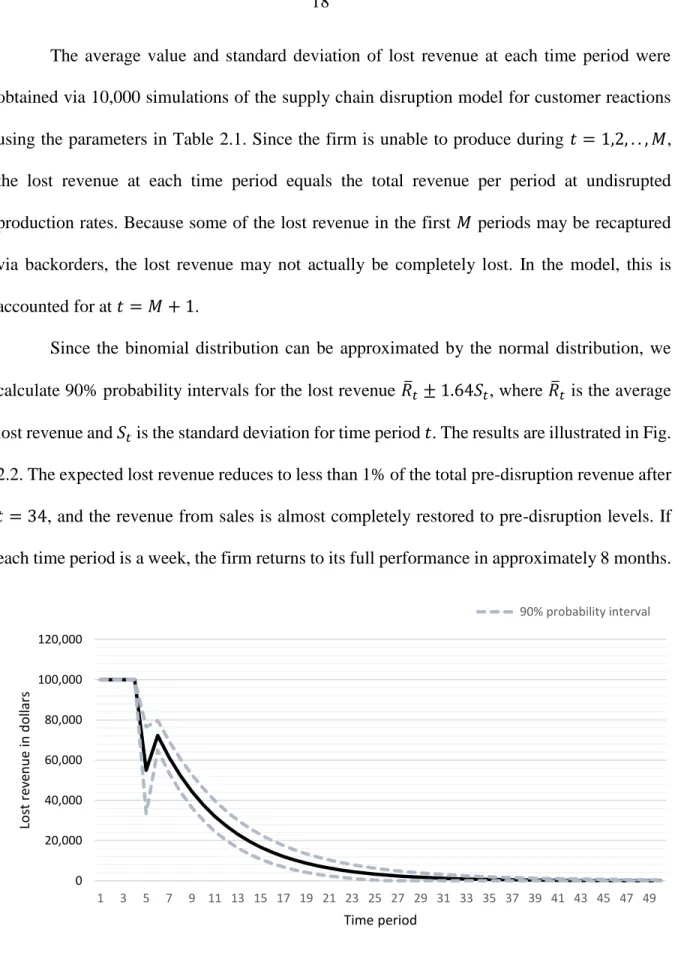
The average value and standard deviation of lost revenue at each time period were obtained via 10,000 simulations of the supply chain disruption model for customer reactions using the parameters in Table 2.1. Since the firm is unable to produce during 𝑡 = 1,2, . . , 𝑀, the lost revenue at each time period equals the total revenue per period at undisrupted production rates. Because some of the lost revenue in the first 𝑀 periods may be recaptured via backorders, the lost revenue may not actually be completely lost. In the model, this is accounted for at 𝑡 = 𝑀 + 1.
Since the binomial distribution can be approximated by the normal distribution, we calculate 90% probability intervals for the lost revenue 𝑅̅𝑡± 1.64𝑆𝑡, where 𝑅̅𝑡 is the average lost revenue and 𝑆𝑡 is the standard deviation for time period 𝑡. The results are illustrated in Fig. 2.2. The expected lost revenue reduces to less than 1% of the total pre-disruption revenue after
𝑡 = 34, and the revenue from sales is almost completely restored to pre-disruption levels. If each time period is a week, the firm returns to its full performance in approximately 8 months.
Fig. 2.2. The firm’s expected lost revenue per period from the supply chain disruption.
0 20,000 40,000 60,000 80,000 100,000 120,000 1 3 5 7 9 11 13 15 17 19 21 23 25 27 29 31 33 35 37 39 41 43 45 47 49 Lo st re ve n u e in d o llars Time period 90% probability interval
As depicted by the probability interval, there is a 5% probability the lost revenue will be less than $1,000 within 24 periods and a 5% probability the lost revenue will be greater than $1,000 for at least 42 time periods. The expected lost revenue is at its maximum value for the first four periods, which is equal to the total pre-disruption revenue per period and then drops from $100,000 to $55,000. The downward spike in the expected lost revenue is due to the backorders. The lost revenue at𝑡 = 5 has a 5% probability of being as low as $33,444, which would occur if many customers return with backorders. If very few customers return with backorders, the lost revenue could be $76,556, which is the 95% upper bound for lost revenue in that time period. At time 𝑡 = 6, the expected lost revenue increases to $72,250 and then gradually decreases over time as the firm recovers from the disruption.
4.2 Lost revenue without backorders
Certain disruptions may not allow for backorders. For instance, a restaurant could be closed for a period of time because of food poisoning, and when it reopens, backorders are not realistic because the delivered product is a service that cannot be backordered. We can assign
𝑞 = 0 in the simulation model to reflect such a situation. Fig. 2.3 illustrates this scenario without backorders. Here, the expected cumulative lost revenue is higher because of the lack of backorders.
Fig. 2.3. The firm’s expected lost revenue without backorders.
4.3 Customers with varying demand
The assumption that each customer buys exactly one product may not be valid. This sub-section extends the simulation model to accommodate varying demands from the firm’s customers. The demand from customer 𝑙 is 𝑛𝑙 where 𝑙 = 1, 2, … , 𝑛. We assume each 𝑛𝑙 follows a discrete uniform distribution between 1 and 5, i.e., 𝑛𝑙 ~ 𝑈(1, 5). Backorders are ignored for simplicity. Parameters from Table 2.1 along with a simulation of 𝑛𝑙 ~ 𝑈(1, 5) were used in the model with varying demand from different customers to run 1,000 simulations. The results are illustrated in Fig. 2.4.
The maximum total expected lost revenue is much higher than the previous cases because the total initial demand is more than in the previous cases. The shape of recovery is very similar to the model in section 4.1 because each customer returns with the same probability. The expected lost revenue reduces to less than 1% of the total pre-disruption
0 20,000 40,000 60,000 80,000 100,000 120,000 1 3 5 7 9 11 13 15 17 19 21 23 25 27 29 31 33 35 37 39 41 43 45 47 49 Lo st re ve n u e in d o llars Time period 90% probability interval
revenue after time period 25. This is comparable to the results from the model in sections 4.1 and 4.2. The results might look different if customers returned with different probabilities. For example, perhaps customers with more demand from the firm might be more likely to return because it may be more difficult for these customers to get all of their demand satisfied from the firm’s competitors.
Fig. 2.4. The firm’s expected lost revenue with varying demand from customers
4.4 Risk management insights
A firm can use this model to understand how parameters impact the firm’s expected lost revenue. The results discussed are highly sensitive to the value of 𝑝. As illustrated in Fig. 2.5, the firm recovers more quickly when the probability with which customers are gained back in each period is larger. This makes intuitive sense since firms with loyal customers tend to recover faster. We observe that the downward spike at time 𝑡 = 𝑀 + 1 is directly correlated
0 50,000 100,000 150,000 200,000 250,000 300,000 350,000 1 3 5 7 9 11 13 15 17 19 21 23 25 27 29 31 33 35 37 39 41 43 45 47 49 Lo st re ve n u e in d o llars Time period 90% probability interval
with 𝑝. At 𝑡 = 𝑀 + 1, the cumulative expected number of orders including the backorders is directly proportional to the probability of customers buying from the firm at a given time period after the disruption.
The expected lost revenue in time period 𝑡 = 5 is negative when 𝑝 = 0.4. This negative value represents revenue greater than $100,000 in that period, a trend that continues as the value of 𝑝 increases. Such situations may require the firm to work at overcapacity immediately after reopening to meet the sudden increase in demand, which is an integral part of the firm’s recovery process (Sheffi and Rice 2005). This provides an important insight to the firm’s management that in case of a production shut down, it may need to be prepared to temporarily increase its production capacity after reopening. The model also helps to estimate the maximum production the firm would need in order to meet the demand.
Fig. 2.5. Sensitivity of expected lost revenue to 𝑝.
-40,000 -20,000 0 20,000 40,000 60,000 80,000 100,000 120,000 1 3 5 7 9 11 13 15 17 19 21 23 25 27 29 31 33 35 37 39 41 43 45 47 49 Exp ected los t re ve n u e in d o llars Time period p = 0.15 p' = 0.05 p'' = 0.40
A similar trend can be observed with the sensitivity analysis on 𝑞, as illustrated in Fig. 2.6. The time of recovery remains the same since 𝑝 is constant. This is also an important insight since firms need to think about the likelihood that their customers will place backorders. Accordingly, they can devise suitable production plans.
Fig. 2.6. Sensitivity of expected lost revenue to 𝑞.
Firms can prepare for disruptions by using this quantitative model to estimate the potential loss in revenue due to a shutdown of operations from a supply chain disruption. Moreover, the model can be used to evaluate whether preparation strategies are economical. Investments to reduce the chances of a supply chain disruption itself may not be practical or economically reasonable. In such cases, firms can use the expected lost revenue from the model to decide whether or not investments to reduce the risk of a disruption are cost effective. Preparedness measures can help reduce the probability of a disruption and/or allow the firm to regain more of its revenue following a disruption. Even if the disruption cannot be avoided,
0 20,000 40,000 60,000 80,000 100,000 120,000 1 3 5 7 9 11 13 15 17 19 21 23 25 27 29 31 33 35 37 39 41 43 45 47 49 Lo st re ve n u e in Do llars ($) Time period, i q = 0.5 q' = 0.20 q'' = 0.80
preparedness measures could reduce the shutdown length 𝑀. It is logical to assume that the probability of customers returning depends on 𝑀. Decision makers can make decisions about investing in preparedness measures based on understanding how much revenue will be lost if the disruption occurs as well as the chances of the disruption itself.
For example, the cumulative expected lost revenue in the illustrative example is $536,667. A risk-neutral firm should spend at most $536,667 in preparing for this type of disruption and should spend much less once the probability of a disruption is considered. Investing in risk reduction strategies such as inventory or an additional supplier could reduce the time the firm is closed. The chances of customers returning immediately to the firm are higher if the firm is not closed as long. This would increase the probability p and reduce the cumulative expected lost revenue. In the example, increasing the value of p from 0.15 to 0.2 decreases the total expected lost revenue from $536,667 to $360,000. Strategies that could reduce p from 0.15 to 0.2 are economically wise if these strategies cost less than $176,667, assuming an extremely high probability of disruption.
Conclusions
This chapter proposes a model to quantitatively represent the way customers or the marketplace reacts to a supply chain disruption. The model is used to identify the impact of such an event on the firm’s revenue. From the firm’s perspective, the total expected lost revenue is a measure of the impact of the supply chain disruption and can be analyzed to draw useful insights to manage the risk of such an event.
The results obtained from applying the model serves as an illustration of the usefulness of the model. The simulation of the customer response model allows the firm to anticipate how customers might react to a supply chain disruption. The model can inform decision making to
manage the risks of a supply chain disruption. Insights from the model can reveal how a disruption can affect the firm’s revenue depending on the customers’ decisions and the time a firm takes to recover to its pre-disruption revenue levels. Sensitivity analysis on the model parameters reveals how the probability at which customers return to the firm impacts the recovery time. Firms that expect most of its customers to return with backorders may need to temporarily increase production capacity. Management can use the cumulative expected lost revenue projections to evaluate investments aimed at increasing the firm’s resilience to supply chain disruptions.
References
Arnade, C., Calvin, L., & Kuchler, F. (2009). Consumer response to a food safety shock: the 2006 food-borne illness outbreak of E. coli O157: H7 linked to spinach. Applied Economic Perspectives and Policy, 31(4), 734-750.
Babich, V., Burnetas, A. N., & Ritchken, P. H. (2007). Competition and diversification effects in supply chains with supplier default risk. Manufacturing & Service Operations Management, 9(2), 123-146.
Beach, R. H., Kuchler, F., Leibtag, E. S., & Zhen, C. (2008). The Effects of Avian Influenza News on Consumer Purchasing Behavior: A Case Study of Italian Consumers' Retail Purchases (No. 56477). U.S. Department of Agriculture, Economic Research Service. Chopra, S., & Sodhi, M. S. (2004). Managing risk to avoid supply-chain breakdown. MIT
Sloan Management Review, 46(1), 53.
Christopher, M. (2005). Logistics and Supply Chain Management: Creating Value-Adding Networks (3rd ed.). Harlow, England: Pearson Education.
Ellis, S. C., Henry, R. M., & Shockley, J. (2010). Buyer perceptions of supply disruption risk: A behavioral view and empirical assessment. Journal of Operations Management, 28(1), 34-46.
Hendricks, K. B., & Singhal, V. R. (2005). Association between supply chain glitches and operating performance. Management Science, 51(5), 695-711.
Jüttner, U., Peck, H., & Christopher, M. (2003). Supply chain risk management: Outlining an agenda for future research. International Journal of Logistics: Research and
Applications, 6(4), 197-210.
Kilubi, I., & Haasis, H. D. (2015). Supply chain risk management enablers: A framework development through systematic review of the literature from 2000 to 2015.
International Journal of Business Science & Applied Management, 10(1), 35-54. Lavastre, O., Gunasekaran, A., & Spalanzani, A. (2012). Supply chain risk management in
French companies. Decision Support Systems, 52(4), 828-838.
MacKenzie, C. A., Barker, K., & Santos, J. R. (2014). Modeling a severe supply chain disruption and post-disaster decision making with application to the Japanese earthquake and tsunami. IIE Transactions, 46(12), 1243-1260.
MacKenzie, C. A., Santos, J. R., & Barker, K. (2012). Measuring changes in international production from a disruption: Case study of the Japanese earthquake and tsunami. International Journal of Production Economics, 138(2), 293-302.
Manuj, I., Dittmann, P., & Gaudenzi, B. (2007). Risk management. In J. T. Mentzer, M. B. Myers, & T. P. Stank (Eds.), Handbook of Global Supply Chain Management (pp. 319-336). Thousand Oaks, Calif.: Sage Publications.
Mentzer, J. T., DeWitt, W., Keebler, J. S., Min, S., Nix, N. W., Smith, C. D., & Zacharia, Z. G. (2001). Defining supply chain management. Journal of Business Logistics, 22(2), 1-25.
Nagurney, A., Cruz, J., Dong, J., & Zhang, D. (2005). Supply chain networks, electronic commerce, and supply side and demand side risk. European Journal of Operational Research, 164(1), 120-142.
Nishat Faisal, M., Banwet, D. K., & Shankar, R. (2006). Mapping supply chains on risk and customer sensitivity dimensions. Industrial Management & Data Systems, 106(6), 878-895.
Sheffi, Y., & Rice Jr, J. B. (2005). A supply chain view of the resilient enterprise. MIT Sloan Management Review, 47(1), 41.
Snyder, L. V., Atan, Z., Peng, P., Rong, Y., Schmitt, A. J., & Sinsoysal, B. (2016). OR/MS models for supply chain disruptions: A review. IIE Transactions, 48(2), 89-109. Sodhi, M. S., & Tang, C. S. (2012). Managing Supply Chain Risk. New York: Springer
Science & Business Media.
Stecke, K. E., & Kumar, S. (2009). Sources of supply chain disruptions, factors that breed vulnerability, and mitigating strategies. Journal of Marketing Channels, 16(3), 193-226. Tomlin, B., & Wang, Y. (2005). On the value of mix flexibility and dual sourcing in
unreliable newsvendor networks. (M&SOM), 7(1), 37-57.
Xia, Y., Ramachandran, K., & Gurnani, H. (2011). Sharing demand and supply risk in a supply chain. IIE Transactions, 43(6), 451-469.
Yu, H., Zeng, A. Z., & Zhao, L. (2009). Single or dual sourcing: Decision-making in the presence of supply chain disruption risks. Omega, 37(4), 788-800.
CHAPTER 3. COST-EFFECTIVENESS ANALYSIS OF SUPPLIER PERFORMANCE BASED ON SCOR METRICS
Based on an abstract accepted for presentation at the 2017 IISE Annual Conference
Arun Vinayak, Cameron A. MacKenzie
AbstractA firm may use several metrics to assess a supplier’s performance, including the quality of delivered products, the time it takes to deliver those products, and how quickly a supplier responds to changes in customer demand. Mapping these measures to what a firm ultimately cares about can help a firm select among suppliers. If a firm has little to no experience working with a supplier, a firm may have difficulty in objectively selecting a supplier. This paper presents a framework for supplier performance measurement based on supplier key performance indicators derived from the performance metrics of the Supply Chain Operations Reference model. The framework can be used for supplier selection as well as for supplier performance monitoring as the firm continues to work with the selected supplier. A decision maker in a firm can incorporate his or her own preferences within the presented framework to determine the most preferred supplier and assess the cost effectiveness.
Keywords: Supplier performance evaluation, SCOR model, Multi-objective decision making, Risk analysis, Supply chain.
Introduction
Selecting and evaluating a supplier is a multi-criteria problem that is growing in its scope and importance (Ho et al., 2010; Agarwal et al., 2011). With the availability of latest technology that can be used to monitor, measure, and compare various aspects of a supplier, organizations can benefit from a simple and effective framework for supplier selection using multi-criteria decision-making techniques. Emphasis on the firm’s objectives and business requirements while selecting a supplier will play a critical role in the success of any firm as there is an increased dependency on suppliers due to business initiatives such as outsourcing, globalization, and lean manufacturing. While such focus on the firm’s core values is vital, an effective supplier performance benchmarking framework must be simple and standardized for the use of multiple industries.
The Supply Chain Operations References (SCOR) model developed by the Supply Chain Council (SCC) with inputs from industry leaders presents a comprehensive hierarchical structure of a supply chain’s performance metrics under five core performance attributes: reliability, responsiveness, agility, cost, and asset management efficiency. Fig. 3.1 presents the hierarchy of metrics of levels 1 and 2 for these five core attributes. To ensure balanced decision making in supply chain management, the SCC suggests that supply chain scorecards should contain at least one metric for each performance attribute. Although these five core performance attributes may be mutually exclusive, they are not directly measurable. There are 43 level-1 performance metrics that support these five attributes which would require extensive data gathering and is not practical. Moreover, these metrics in the SCOR model are designed to measure a supply chain’s performance. While SCOR model serves as a comprehensive
reference guide for supply chain performance measurement, there is a need for deriving a set of metrics that most effectively captures the performance of a supplier.
This paper presents a practical tool that simplifies and combines these attributes to account for their relative importance using a systematic process. Key Performance Indicators (KPIs) for the suppliers derived from the SCOR performance metrics enable us to compare different suppliers from a firm’s perspective and understand the risk associated with them. A subset of the SCOR performance metrics are identified and then aggregated using a value-based approach to multi-criteria decision making. An Excel-value-based tool is presented for decision makers from a firm to incorporate their own preferences for carefully evaluating and identifying the best supplier in a rational mode. An illustrative case application of the proposed framework based on real world expertise is also presented that can be referred by analysts or decision makers from the industry to apply the framework in selecting new suppliers or evaluating existing suppliers.
The model adapts the SCOR metrics for reliability, responsiveness, agility, and asset management efficiency by focusing on the most important metrics and constructing a value function based on those metrics. The value function aggregates the attributes into a single measure of effectiveness. The cost of the supplier is separated from the effectiveness measure in order to make trade-offs between the cost and effectiveness of suppliers. Since several of the SCOR metrics concern evaluating activities for material flow, the proposed model is intended for manufacturing supply chains.
31
This paper is organized as follows: a literature review is given in Section 3.2. Section 3.3 presents the model framework along with an overview of the SCOR performance metrics that serve as the basis of the supplier KPIs presented in this paper. Section 3.4 describes an illustrative example. Section 3.5 concludes the paper with recommendations, insights, and conclusions drawn from the study.
Literature Review
Supplier selection has received significant attention in the academia over the past few decades. Moore (2014) defines supplier selection as the process through which firms identify, evaluate and contract with suppliers. Lil (2007) argues that the sole purpose of selection is not to identify suppliers with the lowest prices and the materials at the right time. Rather, the process revolves around all strategic decisions aimed at meeting the company’s long-term goals with less risk. This ensures that selecting the right suppliers dramatically minimizes purchasing costs while at the same time improving corporate competitiveness. Companies pay attention to the product life cycle, advanced manufacturing process, and the complexity of the design and manufacturing process when making supplier selection decisions (Mohammady & Martinez, 2006). Buyers are concerned with the supplier’s willingness to deliver the right quality at the right time, mutual trust between buyer and seller, and the seller’s technical and financial capabilities (Lima-Junior & Carpinetti. 2016).
Based on literature review on multi-criteria decision making techniques in 78 journal papers for supplier evaluation and selection from 2000 to 2008, Ho et al. (2010) identifies Data Envelopment Analysis (DEA) as the most popular approach. Agarwal et al. (2011) also identifies DEA as the most widely applied methodology for supplier selection based on 60
articles from various journals and conferences from 2000 to 2011. DEA is robust approach that mainly focuses on system efficiency and considers suppliers and processes as a system. In DEA, optimal weights to maximize the efficiency or performance rating of a supplier is calculated using the outputs (e.g. delivery performance, quality, etc.) and inputs (costs). Researchers (Weber, 1996; Braglia & Petroni, 2000; Songhori et al., 2011) conclude that significant benefits to a firm such as reductions in costs, time, and quality can be achieved if inefficient vendors can become DEA efficient. Moreover, supplier selection itself can be carried out based on DEA efficiency of available suppliers. Ho et al. (2010) argue that suppliers can easily get confused by its input and output criteria. The linear programming nature of DEA also assumes that the most effective suppliers are those that are able generate more outputs by using less inputs (Murkherjee, 2017). This is one of the main disadvantages of using DEA (Ho et al., 2010).
On the other hand, based on a review of multi-criteria decision making approaches for green supplier selection in literature from 1997 to 2011, Govindan et al., (2013) concludes that Analytical Hierarchy Process (AHP), a less data intensive and structured method for multi-objective decisions, is the most widely used approach. Basnet (2002) points that unlike other methods, AHP is easy to use, highly flexible and can be used in a wide range of fields. Furthermore, the method can be used to make a consistent decision with respect to multiple qualitative and quantitative criteria (Huan, Sheoran &Wang, 2004). Suppliers could use the combined approach of AHP and Quality Function Deployment (QFD), a management tool that provides a visual connective process to help teams focus on the needs of the customers throughout the total development cycle of a product or process (Moore, 2014; Bouchereau & Rowlands, 2000). When using this combination, the best supplier is assumed to be one that can
efficiently meet most of the buyer requirements (Basnet, 2002). The QFD model is similar to the Simple Multi-attribute Rating Technique (SMART) which helps major decision-makers in the purchasing company to account for factors that are both qualitative and quantitative (Ho et al. 2010). Unlike QFD, the SMART model can structure the supplier’s system and the environment into components that interact with each other to measure and regulate various effects of system errors.
The SCOR model is one of the most promising models for supply chain strategic decision making (Ravindran, 2013). Established in 1996, the model is a re-engineering, benchmarking, process measurement and best practice analysis to be used in supply chain as an integral modelling. SCOR works on the principle of aligning supply chain management practices as well as filling the gaps in supply chain (Lima-Junior and Carpinetti, 2016). Also, the model strives to improve the use of network modelling tools to support management decision and can be integrated with multi-criteria decision-making techniques. Due to this reason researchers agree the SCOR model remains the most effective individualized approach of supplier chain performance measurement given that it can produce better results on its own, compared to other models (Huang & Keskar, 2007; Huan et al., 2004; Kocaoğlu et al., 2013; Lima-Junior et al., 2016).
Integrated and individualized supplier selection methods are significant as they aid suppliers to select the most suitable and efficient suppliers. Using supplier selection methods ensures that companies get to work with the best suppliers who can effectively meet their specific demands. Supplier efficiency not only focuses on cost and ability to deliver quality goods at the right time but also on other equally important factors such as trust, financial capability and supplier’s past reputation. However, there is a lack of alignment in the existing
literature between supplier selection and supply chain strategic decision making as researchers overly emphasized the use of quantitative optimization models in supplier selection (Huang & Keskar, 2007). Hence, there is a pressing need for researchers to fill this gap. Firms should evaluate the expected level of supplier performance along with cost before selecting the most suitable one.
Lastly, there is a need to introduce more models that use value-focused multi-criteria decision-making techniques to address the problem of supplier selection. This is because the technique can integrate the supplier’s structure and capabilities with the requirement of a firm. In the existing literature in supplier selection, methods such as DEA are chosen over value-based techniques since the latter requires more involvement of the decision maker (Seydel 2006). But from a practical perspective, identifying the right objectives and KPIs with the involvement of the decision makers is most important to a firm when compared to computationally intelligent methods to optimize supplier selection. The objective of this chapter is to improve the quality of supplier selection process in the industry by presenting a framework, based on existing multi-criteria decision-making techniques, that provides insights on the trade-offs, increases confidence (or highlight the risk) in the decision, and document the process. The presented framework can be potentially used by firms to evaluate new suppliers using their supplier selection phase with the easy to use Excel tool.
Methodology
This section defines a framework to help a firm select a supplier. The framework is based on the SCOR model which proposes a set of 43 metrics. The SCOR model provides a framework from which to construct a multi-criteria value model that aggregates these metrics
into a single number that describes the effectiveness of a supplier. This section reviews the SCOR performance metrics, translates the SCOR model to an objectives hierarchy, and describes the value functions and weights needed to quantify supplier effectiveness.
3.3.1 Overview of SCOR Performance Metrics
The SCOR model, first developed by the SCC in 1996, is a very promising model for supply chain strategic decision making (Huan et al., 2004). It allows firms to perform a very thorough fact-based analysis of all aspects of their supply chain by providing a complete set of process details, performance metrics, and industry best practices. SCOR identifies five core supply chain performance attributes with 10 level-1 or strategic metrics and 43 level-2 metrics as shown in Fig. 3.1. Below is a summary of the SCOR performance metrics as defined by the Supply Chain Council in SCOR model reference documentation revision 11.0:
Reliability: Reliability describes the ability to perform tasks as expected. This attribute focuses on predicting the outcome of a process. The level-1 metric associated with reliability is perfect order fulfilment, which can be defined as the percentage of orders meeting delivery performance with complete and accurate documentation and no delivery damage. Perfect order fulfilment is further broken down into: percentage of orders delivered in full, delivery performance to customer commit date, documentation accuracy, and perfect condition.
Responsiveness: Responsiveness describes the speed at which tasks are performed in a
supply chain. This is measured by the order fulfillment cycle time, which is the average cycle time to fulfil customer orders. The order fulfillment cycle time is composed of cycle times for the source, make, deliver, and delivery retail.
Agility: Agility describes the ability of a supply chain to respond to marketplace changes to gain or maintain competitive advantage. The three level-1 metrics associated with agility are: Upside supply chain flexibility is the amount of time it takes a supply chain to respond to an unplanned 20 percent increase in demand without service or cost penalty. Upside supply chain adaptability is the quantity of increased production a supply chain can achieve and sustain for 30 days. Downside supply chain adaptability is the reduction in order quantities sustainable at 30 days prior to delivery with no inventory or cost penalties. Value at risk is a popular risk metric widely used by the finance industry to understand the risk exposure of a trading portfolio based on historic volatility.
Cost: In the context of supply chain performance measurement, SCOR model describes
cost as the operational costs of various processes in a supply chain. This is an internally focused attribute that is measured by the total cost to serve in monetary unites as a sum of planning cost, sourcing cost, material landed cost, production cost, order management cost, fulfillment cost, and returns cost.
Asset Management Efficiency: Asset management efficiency is the ability to efficiently
utilize assets. It is associated with three level-1 metrics:
o Cash-to-cash cycle time is the time it takes for a company to turn cash spent on raw materials to inventory and back into cash. It is widely used measure of how a company manages its working capital assets and is calculated as:
𝐴𝑀. 1.1 = [𝐼𝑛𝑣𝑒𝑛𝑡𝑜𝑟𝑦 𝐷𝑎𝑦𝑠 𝑜𝑓 𝑆𝑢𝑝𝑝𝑙𝑦]
+ [𝐷𝑎𝑦𝑠 𝑆𝑎𝑙𝑒𝑠 𝑂𝑢𝑡𝑠𝑡𝑎𝑛𝑑𝑖𝑛𝑔] – [𝐷𝑎𝑦𝑠 𝑃𝑎𝑦𝑎𝑏𝑙𝑒 𝑂𝑢𝑡𝑠𝑡𝑎𝑛𝑑𝑖𝑛𝑔] 𝐼𝑛𝑣𝑒𝑛𝑡𝑜𝑟𝑦 𝐷𝑎𝑦𝑠 𝑜𝑓 𝑆𝑢𝑝𝑝𝑙𝑦: The amount of inventory (stock) expressed in days of sales.
𝐷𝑎𝑦𝑠 𝑆𝑎𝑙𝑒𝑠 𝑂𝑢𝑡𝑠𝑡𝑎𝑛𝑑𝑖𝑛𝑔: The length of time from when a sale is made until cash for it is received from customers. In other words, number of days needed to collect on sales, or accounts receivable expressed in days.
𝐷𝑎𝑦𝑠 𝑃𝑎𝑦𝑎𝑏𝑙𝑒 𝑂𝑢𝑡𝑠𝑡𝑎𝑛𝑑𝑖𝑛𝑔: The length of time from purchasing materials, labor and/or other resources until cash payments must be made. By maximizing this number, the company holds onto cash longer, increasing its investment potential.
o Return on supply chain fixed assets is the return an organization receives on its invested capital in supply chain fixed assets and is calculated as:
𝐴𝑀. 1.2 =([𝑆𝑢𝑝𝑝𝑙𝑦 𝐶ℎ𝑎𝑖𝑛 𝑅𝑒𝑣𝑒𝑛𝑢𝑒] – [𝑇𝑜𝑡𝑎𝑙 𝐶𝑜𝑠𝑡 𝑡𝑜 𝑆𝑒𝑟𝑣𝑒]) [𝑆𝑢𝑝𝑝𝑙𝑦 𝐶ℎ𝑎𝑖𝑛 𝐹𝑖𝑥𝑒𝑑 𝐴𝑠𝑠𝑒𝑡𝑠]
Supply Chain Revenue is different from Net Revenue which could include revenue from sources other than the supply chain, such as investments, leasing real estate, court settlements. o Return on working capital is a measurement of the magnitude of investment relative
to a company’s working capital position versus the revenue generated from a supply chain and is calculated as:
𝐴𝑀. 1.3 = ([𝑆𝑢𝑝𝑝𝑙𝑦 𝐶ℎ𝑎𝑖𝑛 𝑅𝑒𝑣𝑒𝑛𝑢𝑒] – [𝑇𝑜𝑡𝑎𝑙 𝐶𝑜𝑠𝑡 𝑡𝑜 𝑆𝑒𝑟𝑣𝑒]) ([𝐼𝑛𝑣𝑒𝑛𝑡𝑜𝑟𝑦] + [𝐴𝑐𝑐𝑜𝑢𝑛𝑡𝑠 𝑅𝑒𝑐𝑒𝑖𝑣𝑎𝑏𝑙𝑒]– [𝐴𝑐𝑐𝑜𝑢𝑛𝑡𝑠 𝑃𝑎𝑦𝑎𝑏𝑙𝑒])
3.3.2 Objectives Hierarchy and Attributes
An outline of the proposed approach to support the supplier performance evaluation is presented in Fig. 3.2. The approach detailed in Wall & MacKenzie (2013) for multi-criteria decision making and cost effectiveness analysis (CEA) is applied to supplier selection to generate a set of KPIs based on the SCOR performance metrics. The proposed methodology provides managers in a firm with an easy tool that can be used to incorporate their own preferences for carefully evaluating and identifying the best supplier.
Figure 3.2: The proposed approach
First, an objectives hierarchy is developed based on the KPIs derived from the SCOR performance metrics. As depicted in Fig. 3.3, the overall objective is to maximize supplier effectiveness, and this objective is divided into five sub-objectives: maximize reliability, maximize responsiveness, maximize agility, minimize cost, and maximize asset management efficiency.
Although the cost of a supplier is a very important factor in supplier selection, cost is separated from effectiveness in order to focus on the benefits of selecting a supplier and then comparing those benefits with the cost. This approach can also help alleviate the potential issue of a decision maker adjusting the supplier’s effectiveness in order to justify a lower or higher cost (Williams & Thompson, 2004). Cost is defined as the total cost associated with doing business with a supplier. Cost is excluded from the objectives hierarchy and considered in the final step of the methodology for CEA.
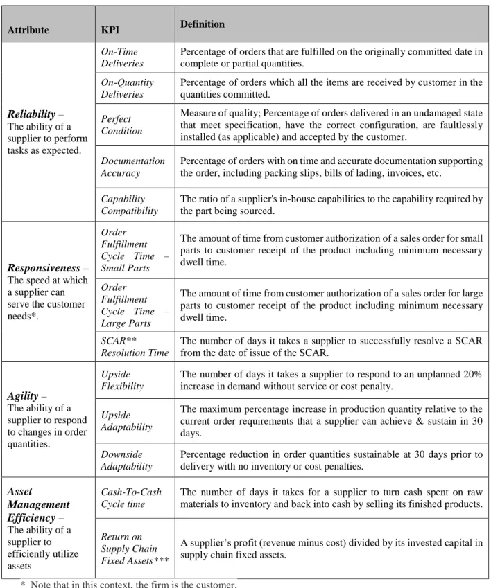
We identify 13 attributes based on the SCOR performance metrics (Fig. 3.4). The presented methodology is generic and the objectives hierarchy can be modified with other KPIs
derived from the SCOR model depending on the firm or the industry. The selected indicators for the framework presented in this paper are shown in Table 3.1. As for the definition of KPIs, the SCOR model has provided with complete definitions for references in the context of an overall supply chain. However, to suit the context of supplier selection as opposed to supply chain performance evaluation, new definitions for the metrics or KPIs are presented in Table 3.1. During the application of this framework, these definitions could be altered based on interviews and discussion with management and staff of the case company. During the process of supplier selection, the KPIs and their definitions (after any necessary alterations) must be sent to each of the suppliers under consideration so that they can submit their estimated KPI values based on their capabilities.