The Price of Diversifiable Risk in Venture Capital and Private Equity
(Article begins on next page)
The Harvard community has made this article openly available.
Please share
how this access benefits you. Your story matters.
Citation
Ewens, Michael, Charles Jones, and Matthew Rhodes-Kropf. "The
Price of Diversifiable Risk in Venture Capital and Private Equity."
Review of Financial Studies 26, no. 8 (August 2013): 1854–1889.
Published Version
doi:10.1093/rfs/hht035
Accessed
February 19, 2015 4:07:11 PM EST
Citable Link
http://nrs.harvard.edu/urn-3:HUL.InstRepos:12534951
Terms of Use
This article was downloaded from Harvard University's DASH
repository, and is made available under the terms and conditions
applicable to Open Access Policy Articles, as set forth at
http://nrs.harvard.edu/urn-3:HUL.InstRepos:dash.current.terms-of-use#OAP
The Price of Diversifiable Risk in Venture Capital and Private
Equity
∗ Michael Ewens† Charles M. Jones‡ Matthew Rhodes-Kropf§ February 19, 2013∗We thank Larry Glosten, Alexander Ljungqvist, Steven Kaplan, Ramana Nanda, Mike Riordan, Tano Santos, Antoinette Schoar, Per Stromberg, S. Viswanathan and participants at the 2003 American Finance Association meeting, the NYSE-Stanford conference on Entrepreneurial Finance and IPOs, the Yale con-ference on Entrepreneurship, VC and IPOs, and the New York University concon-ference on Entrepreneurship, VC and IPOs for their comments. We are grateful to The Eugene M. Lang Entrepreneurship Center for financial support. Special thanks go to Jesse Reyes and Thomson Venture Economics, who provided the Venture Economics data and to Maryam Haque and Brendan Hughes of Dow Jones who provided LP Source. All errors are our own.
†Ewens: Carnegie Mellon University, Tepper School of Business 5000 Forbes Ave Pittsburgh, PA 15213, mewens@cmu.edu
‡Jones: Columbia University, Graduate School of Business, New York, NY 10027, cj88@columbia.edu §Rhodes-Kropf: Harvard University, Rock Center 313 Boston Massachusetts 02163, mrhodeskropf@hbs.edu
Abstract
This paper explores the venture capital (VC) market and extends the standard principal-agent problem between the investor and venture capitalist to show how it alters the interaction between the venture capitalist and the entrepreneur. The nature of the three way interaction results in a correlation between total risk and investor net of fee returns. Thus, we show how and why diversifiable risk should be priced in VC deals even though investors are fully diversified. We then take our theory to a unique data set and show that there is a strong correlation between realized risk and investor returns, as predicted by the theory.
Venture capitalists (often called VCs) are known to use high discount rates in assessing po-tential investments. This may just be a fudge factor that offsets optimistic entrepreneurial pro-jections, but VCs claim to use high discount rates even in internal projections. Furthermore, Cochrane (2005) looks at individual VC projects and shows that they earn large positive alphas, which suggests the use of high discount rates in pricing. In general, VCs seem overly concerned with total risk, especially considering that fund investors are well diversified. Why?
This paper answers this question with a novel theory that links the principal-agent problem to asset prices, with empirical tests of the theory on venture fund data from 1980 - 2011. Our theory extends the principal-agent problem to interactions between the agent and a third party. In the venture capital arena, the principal-agent problem between an investor and a venture capitalist alters the interaction between the venture capitalist and the entrepreneur. We show that it is the entrepreneur who must compensate the venture capitalist for the extra risk that the investor requires the VCs to hold, even though the entrepreneur holds all of the market power in the model. Furthermore, although perfectly competitive investors expect zero alpha in equilibrium, the nature of the three-way interaction results in a correlation between total risk and average return even net of fees. Thus, we show that diversifiable risk can be priced in VC deals, even if the outside investors are fully diversified.
We then take our theory to a large data set of venture capital fund returns and show that there is a correlation between realized risk and investor returns, as predicted by the model: the quartile of VC funds with the greatest idiosyncratic risk has an alpha of 2.55% per quarter, while the lowest quartile has a per quarter alpha of -1.6%.
The trade-off between risk and incentives is a classic feature of contracts. Much of the work on this aspect of the principal-agent problem has focused on either the optimal contract (for example see Holmstrom and Weiss (1985) or Holmstrom and Milgrom (1987)) or on the attempt to see the resulting trade-offs empirically (see Prendergast (1999) for a survey). Our main contribution is to examine both theoretically and empirically the effect of the principal-agent problem on equilibrium asset prices. The VC market is the ideal arena to examine the economic significance of the principal-agent problem, because the investing principals do not have the time or skill to
become overly involved in fund management (and could potentially lose their limited liability status). Furthermore, we can see outcomes, in the form of returns, that are potentially affected by the principal-agent problem.
To bring the principal-agent problem to asset prices we develop a simple yet novel model. The market is characterized by entrepreneurs with ideas, and outside investors who are well-diversified, but have little ability or time to screen and manage potential investments. Investors hire VCs who have considerable expertise in assessing and overseeing entrepreneurial ideas.1 Typically VCs have little capital of their own, so they are in essence money managers, helping investors supervise their investments. Because of standard incentive problems, VCs receive an interest in the firms they fund. They are unable to monetize their holdings and are instead forced to hold a substantial amount of their wealth in the form of these contingent stakes. Furthermore, significant time is required to oversee an investment, which means that a VC can manage only a few investments. Thus VCs hold considerable idiosyncratic risk and must be compensated for bearing this risk.
The standard principal-agent problem ends here. If VCs were simply compensated by the principal for the services they provide and the risk they bear, then fund returns net of VC fees, earned by well-diversified investors, would be uncorrelated with idiosyncratic risk. Investors would compete away excess returns, resulting in zero net alphas.2
In this paper, we go one step further, studying the impact of the investor-VC problem on negotiations between the VC and the entrepreneur. The sequencing is key. VCs and investors strike their bargain first, so the contract is set before the VC actually locates any projects. Thus, the investor-VC contract compensates the VC for the expected risk in the portfolio and not the realized risk.3
The VC, with contract in hand, now negotiates with an entrepreneur. He does not care about
1VCs are thought to have a number of skills relating to the funding and nurturing of new companies. For example, see Hellmann and Puri (2002), Hsu (2004),Kaplan, Sensoy, and Stromberg (2009), Sorensen (2007)), and Ewens and Rhodes-Kropf (2012).
2
It is important to distinguish between gross returns on VC investments and net returns to investors. VC fees of any sort drive a wedge between these two. To get to zero average alphas on net returns, gross expected returns must exhibit positive alphas. Thus, Cochrane’s (2005) finding that individual VC investments earn positive alphas should not be surprising and need not imply that outside investors earn excess returns.
the average risk, but only cares about the risk in the project being considered. All else equal, if this project has greater than average risk then the VC requires a larger return to invest. The contract with the investor is set, so the VC requires the entrepreneur to provide a price reduction on the deal that justifies his personal level of risk. However, this price reduction also benefits the outside investors. Thus, this ‘externality’ requires the entrepreneur to give up more than the amount necessary to just compensate the VC. As a result, higher than expected risk projects earn investors higher returns on average and lower than expected risk projects earn investors lower returns, even though on average investors earn zero alphas.
Thus, if our model is correct, fund returns net of fees could have zero alphas but should still be correlated with ex post total risk! We show formally that this result would not arise if there were no principal-agent problem. Even if, say, VCs must work harder to oversee higher risk firms (and thus demand higher fees), without a principal-agent problem investors’ net returns would not depend on risk. Thus, this surprising prediction canonly be tested with VC investment fund returns net of fees, and this key prediction distinguishes our model from others.
We use newly available data on VC and buyout fund returns to test our model. Although our theory focuses on venture capital, we examine both VC and buyout data because out thoery should apply to any market in which agents hold idiosyncratic risk and thus should also impact all private equity returns to some extent. We combine fund performance data – cash flows and net asset values – from Venture Economics, LP Source, and Preqin. Our data cover a significant fraction of the US venture capital and buyout fund universe from 1980 to 2007. In our sample the average buyout fund has a value weighted IRR of 14% and a beta of 0.72 and an alpha of 4%, and the average venture capital fund has a value weighted IRR of 15% and a beta of 1.24 and a zero alpha.
We use this data to provide evidence that idiosyncratic risk is priced, even in net fund returns. We measure idiosyncratic risk and find that funds with higher realized risk have higher averagenet
returns, exactly as predicted by the model. The results are robust to a series of robustness checks that address cross-sectional differences in fund such as vintage year and investment stage. Thus we find support for the theory - higher idiosyncratic risk funds tend to produce higher returns.
1.
The Principal-Agent Problem
The trade-off between risk and incentives is a classic issue between a principal and an agent. Because the principal does not have perfect information about the agent’s types and/or complete information about the agent’s actions, the principal-agent contract must leave the risk-averse agent with too much risk relative to the first-best solution. The standard problem is that an agent could be a bad type or that an agent must take an action that is costly and unverifiable, such as expending effort. To combat either problem, the principal commits to a contract where the agent’s payoff depends on an observable output.4 If output is subject to shocks that are beyond the agent’s control, then these contingent contracts impose risk onto the agent.
In our model, the venture capitalist is an agent who must be compensated for the opportunity cost of his time. Due to the investor’s (principal’s) lack of information about the type of the VC or the VC’s actions, the VC’s compensation must depend on the returns of his chosen projects. This matches reality, as the standard compensation scheme in private equity and VC is a fixed payment (typically near 2% of the fund per year) and a fraction of the return above some benchmark. Since the VC has limited wealth, a significant portion of his wealth is the present value of his portion of the project returns.5,6 The VC must invest significant time and effort (including board meetings, meeting with management/customers/suppliers, understanding the market, etc.) to help a project realize its value. Therefore, a VC can only manage a limited number of investments. Gompers and Lerner (1999) note that funds typically invest in at most two dozen firms over about three years. In addition, a VC’s expertise may be limited to a particular sector or industry, which means that the VC may remain exposed to sector risk no matter how many projects he selects. Even if a VC can diversify across the entire VC industry, he may not be fully diversified because
4
Holmstrom and Ricart i Costa (1986) offer the idea that even if contracts do not explicitly depend on output, principals use the outcome of the agent’s decision as a signal of the agent’s quality. Since principals promote the high quality agents (they cannot commit to provide full insurance), agents hold risk and their incentives are distorted.
5In practice, when VCs have significant wealth, they are typically required to invest a large fraction of it (perhaps 30-70%) in the fund to show that they “believe” in what they are doing. In other words they must invest in the fund either as a costly signal that they are good or to ensure greater effort.
6
Furthermore, the VC’s ability to raise future funds depends on the success of his first fund (See Kaplan and Schoar (2005) and Gompers (1996). Chevalier and Ellison (1997) also look at the same issue in mutual funds). Therefore, the VC’s future income stream depends on the success of the fund. This compounds the effect of any idiosyncratic risk held by the VC. This idea is similar to Holmstrom and Weiss (1985) who focus on future career concerns rather than specifically contingent contracts.
all VC projects may contain a correlated idiosyncratic risk component. For these reasons, the VC is exposed to significant idiosyncratic risk.7
Why not just combine a large number of VC investments into one much larger fund and compensate the VC based on total fund performance? The answer is that this would eliminate the link between a venture capitalist’s compensation and his chosen projects. If the principal-agent problem were due to costly effort, VCs would exert too little of it. Said another way, the principal-agent problem remains regardless of how VC investments are aggregated into funds, so removing risk from the VC is not optimal. Furthermore, with aggregation VCs may still hold idiosyncratic risk because even in a larger fund the individual VC’s career would depend on the projects he chooses rather than the overall portfolio.
Our theory says that prices should be low in VC and private equity even if there is intense competition among VCs for projects. Prices get bid up until the VC is just indifferent, but this price is still below the price implied by, say, the CAPM. Since the VC needs to be compensated, gross expected returns on the venture capital investment are higher than the factor risks would suggest.
Since VCs correctly use a higher discount rate to evaluate projects, some projects are not taken that are positive NPV based on factor risk alone. This is in line with earlier work, as the principal-agent problem has consistently been shown to distort investment. In papers such as Holmstrom and Ricart i Costa (1986), and Harris, Kriebel, and Raviv (1982) principal-agent problems lead to underinvestment by the principal. In papers such as Holmstrom and Weiss (1985) the agent’s investment choice is distorted. However, none of these papers explicitly consider prices. In our model, the necessary pricing of idiosyncratic risk can result in the decision not to invest. The principal-agent problem leads to a contract that may cause a competitive VC and an entrepreneur to be unable to find a price to fund an otherwise profitable project.
Even though the VCs correctly use higher discount rates, the well-diversified investors who
7Meulbroek (2001) expresses a related idea that managers of internet firms who receive stock cause a deadweight loss because outsiders can diversify. In our model, we assert that the relevant outsider is probably a venture capitalist who cannot diversify either. We agree that there is a deadweight loss relative to first-best, and we show that it manifests itself in venture capital asset prices.
give money to the VCs do not earn excess returns in expectation. The contract between the investor and VC awards part of the fund’s return to the VC. Since the investor can easily diversify, competition among investors means that they earn zero alphas on average.
Our extension of the principal-agent theory to the interaction between the VC and en-trepreneur produces a novel prediction that is not easily explained by other potential theories. The VC and the investors negotiate their contract before the VC locates the eventual fund invest-ments. Thus, the contract is negotiated based on the expected level of risk. However, once the VC identifies profitable projects, the actual amount of risk may differ from the expected amount. Since the realized level of risk cannot be verified by the investor, the contract cannot depend on the actual risk. When the actual risk is higher than the ex ante expectation, the VC demands more from the entrepreneur to compensate him for the additional risk. Therefore, although in-vestors receive zero alphas on average, returns net of fees are positively correlated with ex post
idiosyncratic risk.
If the principal-agent problem truly has economic significance it is here in the VC market that we should see its impact. The prediction from our model is not easily explained by other potential theories, and its presence in the data gives us some confidence that the principal-agent problem does indeed affect prices and returns.
2.
The Model
The model has three participants: investors, venture capitalists and entrepreneurs. Investors are willing to invest a total ofI dollars into a fund that invests in N projects. Each project receives
I/N dollars. Entrepreneurs have project ideas but need some help and guidance to realize the value of their ideas. Their ideas produce random output of (1 +Ri)I/N if they are overseen by a skilled, involved investor and zero if they are not. Even with guidance, the projects have both systematic and idiosyncratic risk and an uncertain return Ri =αi+βiRm+εi,whereRm is the return on the market andεi is idiosyncratic risk. There is also a risk free asset with zero return, and the single-period CAPM holds for all traded assets. The projects may be positive or negative
NPV, αi R0. Ri and Rm are jointly normal, with E[εi] = 0, E[εiRm] = 0,and E[εiεj] = 0, for all project pairs i and j.8 Therefore, the expected return on a project is µi = 1 +αi+βiE[Rm] with variance σ2i =βi2σm2 +σ2εi. We let the subscripts iand j represent particular projects from the space of all possible projects, Ω.
Entrepreneurs have no money. Investors have money, but do not have the skill to determine whether a project is positive or negative NPV, or to manage a project. The VCs, also with zero wealth9, have the ability to locate and successfully manage projects, and determine the characteristics of those projects, αi, βi and σεi (the investor knows the distribution of these
parameter values but cannot verify a particular project’s characteristics). In order to successfully manage a project, a VC must exert effort with an opportunity cost of evc (as in Grossman and Hart (1981)). The effort of the VC is unverifiable. Therefore, the VC must be compensated in order to manage investments for the investors, and this compensation must provide the VC with the incentive to provide effort.
Managing a project is a time consuming process. Therefore, initially we assume the VC is unable to successfully manage more than N projects.10 However, in Section 4. we relax this assumption and examine the VC’s incentives to choose more or fewer projects.11
Investors, venture capitalists, and entrepreneurs are all risk-averse and require compensation for the risk that they hold. However, investors have enough wealth outside the fund that they are well diversified and therefore only require returns for their undiversifiable or factor risk.
The timing of the model is a three-stage game. In the first stage, the investors and VC form a fund and agree on a contract to govern their relationship. In the second stage, the VC negotiates the payoff schedule that the entrepreneurs give up to get I/N dollars from the fund.
8
E[εiεj] = 0 is not required, but it simplifies the exposition of the results. The appendix drops this assumption. 9This assumption ensures that the VCs compensation is a significant fraction of the VC’s wealth and therefore its impact cannot be diversified away with outside wealth. In actuality VCs with prior significant wealth are often required to put between 30-70% of their total net worth in their fund. We argue that this signals their competence and ensures their effort by reducing their ability to diversify.
Limited wealth also ensures that the VC can only receive a positive payoff from the fund.
10In addition, the typical VC contract restricts the amount of money that can be invested in one investment. Therefore, since the size of the fund is given, the VC must invest in a minimum number of projects.
11The principal-agent problem that surrounds many aspects of project choice is an interesting problem studied by Dybvig, Farnsworth, and Carpenter (2010), Kihlstrom (1988), Stoughton (1993) and Sung (1995). Here we focus only on the choice of risk.
The investments also occur in the second stage. In the final stage, project values are realized and payoffs are distributed.
We assume competition among investors gives VCs all the bargaining power when negotiating with LPs. Similarly, the competition among VCs for the scarce positive NPV entrepreneurial projects gives all the bargaining power to the entrepreneur. Since all rents accrue to the en-trepreneur, this minimizes the chance of finding any positive alphas in equilibrium.
Due to the principal-agent problem between the investor and VC, the optimal contract between them depends on the realized value of the projects.12 Further, due to the need to share risk between the investor who can diversify and the entrepreneur who cannot, the optimal contract between the fund and the entrepreneur must depend on output.13 The results of this paper hold as long as the contracts depend on the output of the projects. However, in order to achieve simple closed form solutions we assume that both contracts are equity contracts. Thus, the negotiations are first over φ, the fraction of the fund given to the VCs, and then over the fraction, θi,of the companyI/N dollars will purchase.14
Holmstrom and Milgrom (1987) show that a linear sharing rule is optimal when effort choice and output are continuous, but monitoring by the principal is periodic. The idea is “that optimal rules in a rich environment must work well in a range of circumstances and therefore would not be complicated functions of the outcome” (Holmstrom and Milgrom (1987) p 325). Dybvig, Farnsworth, and Carpenter (2010) show that an option-like contract may be optimal if the agent chooses both effort and a portfolio. Under different conditions different contracts are optimal. We do not want to focus on the actual effort choice (see Gompers and Lerner (1999), Gibbons and Murphy (1992) and, of course, Holmstrom and Milgrom (1987) for interesting work which focuses on the effort decision) and we are not interested in the trade-offs involved in a particular contract.
12
The use of a contract that depends on the performance of the fund can also be motivated with a signaling story. For example, the contract can be used to separate the VCs that are able to accurately screen projects from those who cannot. Those VCs that have no skill would be less willing to take a contract that rewards them only if the fund does well.
13
An output-based contact between the fund and the entrepreneur could also be motivated by a principal-agent problem, or if the VC has more information about the success of the project than the entrepreneur, etc.
14As already mentioned, it is possible that noθ exists that is acceptable to both the VC and entrepreneur. We examine this more thoroughly in a moment.
Instead we simply wish to motivate the use of a sharing rule rather than fixed compensation. In our work we take the form of the contract as given and focus on its implications for asset prices; the implications are the same as long as the contracts depend on the output.
2.1. Benchmark: No Venture Capitalist Needed.
In order to provide a benchmark to compare to the more interesting results to follow, we first consider the pricing when the investors can profitably invest directly in the entrepreneurial projects and projects require no oversight. Thus, for a moment we remove the VC from the problem, but assume that the project is still positive NPV (specifically, we assume the investors can determine and expect to earn theαi,βi andσεi of projecti).
Given this setup, mean-variance preferences plus perfect competition among investors ensures that investors are willing to fund the project as long as αi ≥ 0. That is, investors are willing to fund positive NPV projects, where discount rates are determined using the CAPM. Perfect competition among well-diversified outside investors implies that the entrepreneur retains all the economic rents from the project.
In the absence of a VC, investors fund a project directly. To begin we assume for simplicity that N = 1 (the appendix considers multiple projects). Investors put upI dollars and receive a fractionθi of the firm. The firm’s random payoff is (1 +Ri)I, where, as described earlier, project returns follow the single factor model
Ri=αi+βiRm+εi. (1)
Thus the investors receive θi(1 +Ri)I. This implies that the beta of the investors’ returns with respect to the market return is equal to θiβi.15 Given this setup, the entrepreneur minimizes θi
15Although the concept of beta is scale-independent, a change inθchanges the fraction of the project owned by the investor even though he invests the same amount. Thus, his exposure to the risk of the project changes with the fraction he owns. For example, suppose the investor puts up all of the cash but receives only 75% of the project payoff. An additional 1% return on the project increases the investor’s return by only 0.75%.
subject to giving the investors a fair return:
minθi s.t.
θi(1 +αi+βiE[Rm])I 1 +θiβiE[Rm]
=I, 0≤θi ≤1. (2) The constraint is the expected payoff to the investors discounted at the appropriate CAPM rate, and generates an NPV of exactly zero.
There is only one θi that satisfies the constraint, and it is given by:
θi= (1 +αi)−1, (3) provided thatαi ≥0. Since the fractionθi of the firm is worthI dollars, the so-calledpost-money implied value of the whole firm is Iθi−1 or simply I(1 +αi), which reflects the investment plus the expected value added by taking on this positive NPV project. The so-calledpre-money value of the firm is just the post-money value less the amount contributed by investors, or in this case
Iαi. Thus, all the rents accrue to the entrepreneur.16
2.2. The Venture Capitalist’s Impact on Prices.
Now we address the more interesting case where there is a VC present. As before, the entrepreneur gives up a fraction of the firmθi to the investors, but now the investor gives the VC a fraction of the firm φθi and retains the fraction (1−φ)θi.
The VC is risk-averse with exponential utility over terminal wealth w:
u(w) =−exp(−Aw), (4)
whereAis the VC’s coefficient of absolute risk aversion. If terminal wealth is normally distributed,
16
A simple example will help clarify the terms post-money and pre-money value. If the entrepreneur convinces the investor that his firm/idea is worth $2 million and the investor invests $1 million at that valuation, then the value of the firm pre-money was $2 million and the post-money value is $3 million. These terms are used to make it clear that although the investment increases the value of the firm it does not change the price of the stock (there is more money but also more shares).
then maximizing expected utility is equivalent to max µw− 1 2Aσ 2 w, (5)
whereµw and σ2w are the mean and variance of wealth. This functional form for utility allows for a closed-form solution but does not drive the results. All that is necessary is a risk-averse VC.17
The VC has no other wealth but has outside opportunities that give him a certain payoffevc. Thus, in order to manage potential investments, the VC requires compensation that generates at least as much utility asevc, the opportunity cost of his effort.
We derive the solution using backward induction. Thus, we begin with the second stage negotiations. In the second stage the VC locates a suitable project, determines its characteristics,
αi,βi and σεi,and negotiates with the entrepreneur. As in the benchmark case, the entrepreneur
minimizes the fraction θi.However, this minimization is now subject to providing the VC with utility greater than the opportunity cost of his effort. Thus, the introduction of the VC alters the constraint faced by the entrepreneur from the benchmark case. Formally, the minimization problem is min θi (6) s.t. φθiIµi− 1 2AI 2φ2θ2 iσi2 ≥evc,
whereφ is the predetermined contract between the VC and the investor, σi2=βi2σm2 +σε2i is the total variance of payoffs, and µi= 1 +αi+βiE[Rm] is the expected return on the project.18
The entrepreneur wants to minimize the VC’s and investor’s take subject to the VC’s con-straint, and since the market is competitive, the offered contract provides a certainty equivalent of exactly evc. The binding constraint is quadratic in φ and yields the following expression for
17
The appendix allows for a general risk averse utility function. 18
We assume that forθ ∈[0,1] the VC’s utility increases with θ.Specifically this requiresφIµi−AI2φ2σ2i >0. This eliminates the economically unreasonable (but mathematically possible) outcome that the VC’s utility is improved by decreasing the fraction of the firm he receives.
the share of the company offered to the VC in equilibrium: θ∗i = µi−(µ 2 i −2Aevcσi2) 1 2 AφIσi2 (7)
Note that the model implicitly assumes that the VC has no access to the capital markets. If he could, the VC might want to hedge out his market risk by trading in the market portfolio. Based on our conversations with venture capitalists, we do not believe that such hedging is common, but if the VC were able to eliminate all market risk, pricing would still be affected by idiosyncratic risk rather than total project risk.
Moving back one stage, to the first stage of the model, the VC and the investors must negotiate the equity contract that will govern their relationship. At this stage the VC has not yet located a suitable investment so the characteristics of the investment are not known. However, both the VC and investors can determine the distribution of the subset of projects that the VC would accept in the second stage, Ωvc⊂Ω. Therefore, before an investment has been located investors’ expectations are over the subset of projects Ωvc.19
In negotiating a contract, the VC attempts to maximize his expected utility subject to the investors receiving a fair return in expectation for the risk they hold:
max φ EΩvc[u(w(φ))] (8) s.t. EΩvc θ∗i(1−φ)µiI 1 +θi∗(1−φ)βiE[Rm] ≥I,
As in the benchmark case, the constraint binds because we have assumed perfect competition for VCs and investments. However, the constraint now includes an expectation because the investor does not know the project characteristics when he negotiates with the VC.
In order to get an easy-to-interpret closed-form solution we make the following simplifying assumption. We assume that there are only two equally likely projects within Ωvc, and each
19
The expected returns are not normally distributed because a mixture of normals is not normal. However, the investors are assumed to have mean-variance preferences and the VC’s expected wealth is still normal conditional on a chosen project. Therefore, the investor is willing to accept a contract as long as the expected present value of his return is greater than his investment.
project only differs in its level of idiosyncratic risk σε2i.Thus, the VC receives a different fraction
θ∗i from each project. These assumptions do not drive any of our results and are dropped in the general formulation in the appendix; they simply make clear the effect of idiosyncratic risk. The binding constraint becomes,
θ1∗(1−φ)µ1I 1 +θ∗1(1−φ)β1E[Rm] 1 2 + θ2∗(1−φ)µ2I 1 +θ∗2(1−φ)β2E[Rm] 1 2 =I, (9)
whereµ1 =µ2 ≡µand β1 =β2 ≡β.Solving for φyields20,
φ∗= 1−q 1 (1 +α)θ∗1θ2∗βE[Rm] +161 (θ1∗+θ∗2) 2(1 +α−βE[R m])2+14(θ1∗+θ2∗) (1 +α−βE[Rm]) . (10) There is clearly a solution to Equations (7) and (10).21 However, as developed below there is not necessarily a solution with θ∗ and φ∗ between zero and one. Thus, a deal may be economically impossible.22
2.2.1 What if there were no principal-agent problem?
A central insight of our model is that in pricing and in capital budgeting, the principal-agent problem introduces a wedge between gross returns on investment and net returns to investors. We will show that the size of this wedge varies with the level of idiosyncractic risk and affects expected returns to investors. However, even without a principal-agent problem, there would still be a wedge as long as there are VC fees paid out of the gross returns. Thus, it is important to distinguish which results are due simply to the wedge between gross and net returns, and which results are due specifically to the principal-agent problem. To do this, we develop a parallel model without the principal-agent problem. The formal development of this model can be found in the
20We are only interested in the positive root since q1 16(θ ∗ 1+θ ∗ 2) 2 (1 +α−βE[Rm])2 = 14(θ1∗+θ ∗ 2) (1 +α−
βE[Rm]) the negative root would yieldφ >1,which would not make economic sense. 21
Proof: φ∗(θ∗1, θ2∗) is monotone and for any θ2∗ : φ∗(0, θ∗2) < ∞ and lim θ∗1→∞ φ
∗
(θ1∗, θ∗2) = 1. The inversion of equation (7) is monotone and lim
θ∗
1→0
φ∗(θ1∗)→ ∞and lim θ∗
1→∞
φ∗(θ∗1) = 0. Therefore, single crossing is satisfied and there must be an equilibrium for anyθ∗2 (though not necessarily an economically reasonable one).
22Note that sinceφ∗
appendix, but we provide an overview here.
If there were no principal-agent problem, the VC would still locate projects and negotiate with the entrepreneur for a share of the project, but the investor would rely on the VC to take actions in the investor’s best interest. VC compensation would not need to depend on fund performance. In this case, the VC’s payment would depend on the project’s expected returns (µi) rather than the realized returns. The VC’s compensation must, of course, still be greater than or equal to the opportunity cost of his effort,evc, but the VC would hold no risk.
The effort required from the VC might also depend directly on the variance of the project. For example, if higher risk projects are more costly to evaluate or more costly to oversee, then the VC’s effort can be written as evc(σi2), an increasing function of project variance. Note that even if VC effort depends on the risk, in the absence of the principal-agent problem, the principal can simply agree to a contract that pays the VC more if the required effort is more. Thus, the VC still holds no risk but is compensated more for greater required effort.
We now turn to the implications of our model. Some results hold as long as there is a VC paid out of gross returns, and some are specific to the principal-agent problem. This will allow us to empirically distinguish the principal-agent problem from many other theories.
2.2.2 Theoretical Implications
In what follows, we present the main results in Theorems 1 through 4 and then, in the corre-sponding corollaries we consider the alternative in which there is no principal-agent problem. The corollaries show that Theorems 1 through 3, while interesting, cannot help us empirically distinguish our model. Thus, theorem 4 is the key implication of our model and the theorem we test. All proofs are in the appendix.
Theorem 1 Venture capital gross investment returns have positive gross alphas. Investor returns net of fees have zero alphas on average.
It appears that the investment has expected returns that are too high. On average, this isn’t so. Nobody expects excess returns in this model. The returns above the benchmark case are just enough in expectation to compensate the VC for his services and for the idiosyncratic risk he holds. This is consistent with Cochrane (2005), who finds that individual VC investments earn positive alphas at the project level.
It is interesting to note that relative to the benchmark case with no VC needed, the en-trepreneur must give away too much of the firm in return for the investment. Here, it is the entrepreneur who must compensate the VC for the additional risk that the investor requires the VC to hold even though the entrepreneur has all of the market power in the model. This is because the investor must on average earn a return commensurate with the factor risks or he will not participate in the VC market. Thus, in equilibrium all investment expenses must be borne by the entrepreneur.
Theorem 1 is an important implication of the principal-agent problem. However, this result is not too surprising and cannot help us empirically distinguish our model. As the following corollary shows, Theorem 1 holds in a model without the principal-agent problem.
Corollary 1 Even if there is no principal-agent problem gross investment alphas may still be positive.
Our theory predicts positive alphas before fees. However, as long as VC fees are nonzero, alphas before before fees should be positive. Thus, we cannot use Theorem 1 to test our theory. For example, Cochrane (2005)’s empirical finding of large alphas on VC projects does not provide any evidence of a principal-agent problem. We need more.
Theorem 2 Given any positive NPV project, if the total risk is large enough then the VC does not invest. Furthermore, if the ex ante expected α of the universe of projects that the VC would accept is positive but sufficiently small then the investor does not invest.
Conditional on a contract with the investors, the VC would not be willing to accept some positive NPV projects that have high risk. Furthermore, although (for a given φ) the VC would
be willing to accept some negative NPV projects23with low risk, the set Ωvc must include projects with high enoughα or the investor would be unwilling to provide the VC with a contract at all. Thus, in equilibrium a draw from the set Ωvc (the only investments that will occur) must have a high expected α relative to its total risk.
When a paper claims that the NPV rule is no longer valid, it is important to ask which NPV rule it is and whether a suitably adjusted NPV calculation might restore order. In this context, it is useful to think of the VC’s share of the firm as consisting of two parts. One part is compensation to the VC for his effort, and the other part is compensation to the VC for the idiosyncratic risk that he must hold. The value of the VC’s effort could and perhaps should just be taken out of the net cash flows. This would go part of the way toward restoring the NPV rule. Compensation to the VC for risk is not quite the same, however. In principle, this too could simply come out of the net cash flows, and the NPV rule would be completely restored. But a higher hurdle rate that accounts for the VC’s idiosyncratic risk also makes intuitive sense, because more risk borne by the VC is associated with a higher implied hurdle rate. Gross expected returns on the investment really do have to be higher because of the added risk.
Theorem 2, although interesting, has the same problem as Theorem 1. The following corollary shows that the same result would hold for a model without the principal-agent problem.
Corollary 2 Even if there is no principal-agent problem some positive NPV projects may not get done.
Since VCs use a higher discount rate to evaluate projects, some projects cannot get done that are positive NPV based on factor risk alone. However, it is also the case that compensation that does not depend on fund returns has the same qualitative effect. Therefore, as with Theorem 1, Theorem 2 cannot help us empirically determine if our theory is correct.
23For the VC to choose to invest the VC’s constraint must be satisfied. Givenφ∗
the constraint, φ∗θiIµi− 1
2AI 2
φ∗2θi2σ2i ≥ evc, can be satisfied if the venture capitalist has sufficiently low risk aversion (small A) but
φ∗θiIµi ≥ evc. Since the entrepreneur increases θi until the constraint is satisfied, and the largest θi = 1, the constraint reduces to φ∗Iµi ≥ evc or 1 +αi+βiE[Rm] ≥ evc/φ∗I. Therefore, a VC with sufficiently low risk aversion accepts a negative NPV project as long as the total return is large enough.
Theorem 3 All else equal, the price the entrepreneur receives is decreasing in the amount of idiosyncratic risk. Therefore, gross returns are positively correlated with ex post idiosyncratic risk.
If unavoidable principal-agent problems make diversification impossible, then idiosyncratic risk must be priced. Therefore, VC gross returns should be correlated with total risk, not just systematic risk. Projects with higher total risk should have higher returns.
It might seem that this theorem could help us empirically distinguish our model, since idiosyn-cratic risk is related to returns. However, the following corollary also shows that this prediction could also arise from other simple models. For example, if higher risk projects are more costly to evaluate or more costly to oversee, then even if there is no principal-agent problem the en-trepreneur must pay more to get people to invest.
Corollary 3 Even if there is no principal-agent problem the price the entrepreneur receives may still be decreasing in the amount of idiosyncratic risk.
If high risk projects are more costly to oversee, then the VC must be paid more. The en-trepreneur must give up more of his firm to get investors to invest, and gross returns would be higher for high risk projects. Therefore, Theorem 3 cannot help us distinguish the effect of the principal-agent problem from other models. To do this we must look at net returns.
It might seem that, once we remove the VC’s fees, the net return to investors should be unaffected by idiosyncratic risk, particularly since investors are perfectly competitive. However, the following theorem shows that the return to investors is affected by idiosyncratic risk.
Theorem 4 On average, venture capital investment returns net of fees increase with the amount of ex post idiosyncratic risk, even though investors are well-diversified and face competitive market conditions.
Proof Assuming an economically reasonable equilibrium exists, the net fraction owned by the investors equals θi−θiφ∗.Theorem 3 showed that the fraction given up by the entrepreneur,θi,
varies with idiosyncratic risk, dθi/dσε2i > 0. However, the share taken by the VC, φ
∗, does not
change with the realization ofσε2i because it is determined ex ante before the project risk is known. Therefore, the fraction held by investors is a function ofσ2εi.Thus, the net returns are correlated with realized idiosyncratic risk. Competitive conditions ensure that the expected alpha is zero, but realized alpha is positive on average for high idiosyncratic risk projects and negative for low idiosyncratic risk projects.
This is the most important and most surprising theorem in the paper. We later test this theorem and demonstrate that even though investors earn zero alphas in expectation, net returns are still correlated with ex post idiosyncratic risk. The idea is straightforward: the contract struck between the VC and investor is based on the expected level of idiosyncratic risk. When the realized risk is higher than expected the VC demands more from the entrepreneur to compensate him for the risk. And when the realized risk is lower than expected, competition among VCs means the VC demands less from the entrepreneur. The investor is affected by these demands. That is, the investor makes the required return on average, but earns a positive alpha sometimes and a negative alpha at other times.
This key prediction follows directly from the principal-agent problem. It is surprising on first blush because one would expect that the principal-agent problem would have no effect on returns to well-diversified investors. However, when we consider that the principal-agent problem arises because the investor cannot monitor the VC and must therefore negotiate a contract in advance, we begin to see how the principal-agent problem could affect investor returns. The contract is designed to compensate the VC for the expected risk of the portfolio, but since the VCs invest in so few projects realizations of high and low risk portfolios should happen with some frequency. What happens if the VC locates a surprising number of high risk projects? He negotiates better terms from the entrepreneurs. The externality in this negotiation is that the investor also benefits from the VCs negotiation. This is not internalized by the investor-VC team because their contract is already set. Thus, to receive an investment from the VC the entrepreneur sets a lower price and the investor benefits.
This is the key prediction of our model because it is not easily generated without the principal-agent problem. If, for example, high risk investments had higher costs of investing, or monitoring high risk investments was more costly, then high risk projects would have higher gross returns,
but this would not show up in investors’ returns. The following corollary makes it clear that these results only occur when there is a principal-agent problem.
Corollary 4 Without a principal-agent problem, even when the VC’s compensation depends on idiosyncratic risk, the net returns are independent of the idiosyncratic risk.
Without the principal-agent problem, any excess return required to compensate the VC goes to the VC. Therefore, the investors’ return net of fees just compensates them for their beta risk. Theorem 4 allows us to distinguish between a positive alpha that is simply the result of an uncompetitive market or simply because VC’s require compensation, and a positive alpha that is due to the pricing of idiosyncratic risk. If the principal-agent problem is of true significance in the VC arena, then the investors’ returns should be correlated with risk even though the investors earn no excess returns on average.
3.
Empirical Tests
3.1. Data
We use vintage year performance data from three commercial data providers: Venture Economics (VE), LP Source and Preqin.24 The data cover performance – cash flows and net asset values – for buyouts and venture capital funds from 1980 to the end 2011. Stucke, Harris, and Jenkinson (2011) details the methodology and coverage of Venture Economics and Preqin in detail. LP Source is a dataset of fund performance sourced with public information (similar to Preqin) maintained by Dow Jones. For our analysis, we aim to use the maximum and best information available from all data sources. The Venture Economics data covers fund performance from 1980 - 2002. Stucke (2011) shows that the Venture Economics data stops accurately updating in 2001,
24
so only use fund data from Venture Economics with vintage years on or before 1997 and remove post-2000 fund data. We supplement this data with fund returns from Preqin and LP Source. These two datasets combine to provide fund returns from 1984 to 2011 and vintage years 1982 to 2007. A comparison of both cash flow detail and length of fund time series between Preqin and LP Source led us to default to Preqin when both sources had data on a fund.25 So the final data combines Venture Economics for funds between 1980 and 1997 and the merged dataset of Preqin/LP Source for the remaining vintage years.26 The total number of unique funds by vintage
year and type is shown in Figure 1. The coverage by data source is in Figure 2.
The final dataset of interest includes all buyout and VC funds with at least 16 quarters of returns with a vintage year between 1980 and 2007.27 We are left with 741 buyout and 1040 VC
funds. Although the theory above was developed with venture capital in mind, it applies to any situation with a three way principal-agent interaction. This interaction occurs in private equity more generally although one might expect the results to be less pronounced when investing in areas with less idiosyncratic risk.
Table 1 summarizes the characteristics of the funds in the sample. Venture capital funds are generally older (1992 average vintage year) compared to buyout funds (average 1996). This difference stems from slow growth of new venture funds in the post-2001 era and the large increase in buyouts formed prior to the financial crisis of 2008. Venture capital funds can invest across a range of industries and stages. We have information on the latter, which shows that about 39% make early stage investments. The table presents the fraction of the full sample sourced by each data provider.
Table 1 also reports the average and size-weighted IRRs for both fund types, calculated using the full set of cash flows to liquidation or the end of sample. The average VC fund in the sample has an IRR of 13% and when size-weighted, increases to 15%. These compare to
across-25LP Source cash flow data starts in 2002, although many funds have earlier vintages. 26
We lack significant identifiers of funds in Venture Economics, so we used a very conservative methodology to merge it and the other datasets.
27
The dataset is cleaned by removing obvious data errors and ignoring funds whose values go to zero and back to positive. LP Source had instances of the same fund because multiple LPs were investors. We kept one observation per fund, keeping the fund/LP with the most information.
database averages of 15% and 17% respectively in Harris, Jenkinson, and Kaplan (2012) and 11% in Robinson and Sensoy (2011). Buyout fund IRRs of 13.8% and 14% mostly match the numbers reported in Harris, Jenkinson, and Kaplan (2012). Both sets of fund returns exhibit significant volatility: 30% and 44% annualized for VC and buyouts.
3.2. Estimating Risk and Return
Our main empirical prediction is that average returns are increasing in the amount of idiosyncratic risk. Ultimately, we calculate the root mean squared error (RMSE) from the 3-factor returns model for each fund and form portfolios based on this estimate to test for correlation with returns. Unique features of the data and private equity market limit the use of standard factor models and idiosyncratic risk estimates.
For publicly traded stocks with a complete price history, it is straightforward to estimate both factor loadings and idiosyncratic risk. In a single factor model, for example, idiosyncratic risk is the standard deviation of the residual in the market model regression:
rit=αi+βirmt+εit, (11) where rit and rmt are the excess returns over the risk free rate. This equation can be estimated consistently using a time-series of returns. In the present case, funds themselves report the value of their investments each quarter. If these estimates of value simply have i.i.d. measurement errors, then these errors bias upward the estimates of idiosyncratic risk. The measured residuals would also be negatively autocorrelated, though that is not particularly relevant here. The situation is analogous to bid-ask bounce, and the volatility effects of that particular measurement error are addressed by Roll (1984).
Measurement error is not a problem if these measurement errors are uncorrelated with returns or the true amount of idiosyncratic risk, because we do not care much about the actual level of idiosyncratic risk. As long as measured idiosyncratic risk remains informative about the true amount of idiosyncratic risk, then we can test the theory by testing for a positive association
between measured idiosyncratic risk and returns.
A bigger problem is that funds tend to adjust their net asset values slowly. This impacts our estimate of fund quarterly return which uses changes in reported net asset value (NAV), distri-butions (Dit) and takedowns (Tit). Non-excess quarterly returns are calculated as (N AVit+1+
Dit+1 −Tit+1 −N AVit)/(N AVit). In fact, the National Venture Capital Association provides mark-to-market guidelines that explicitly encourage such conservatism. For example, according to the guidelines, a startup’s value should only be written up if there is a subsequent financing round involving a third party at a higher valuation.
If a fund adjusts its net asset value in a consistent, time-stationary way with a one-period lag, and the measured market return itself has no such lags, then the problem is identical to the nonsynchronous trading problem studied by Lo and Craig MacKinlay (1990) and Boudoukh, Richardson, and Whitelaw (1994), among others. Systematic risk can be measured by projecting on current and lagged market returns and then summing up the estimated slope coefficients to obtain an estimator for beta (see Dimson (1979)):
rit=αi+β0irmt+β1irm,t−1+. . .+β4irm,t−4+εit (12) whererit is the quarterly excess fund return calculated using cash flows and net asset values.28
The variance of the residual in this regression is a monotonic function of the true (unobserved) idiosyncratic risk. More lags can be added to this regression if the fund adjusts its returns with a longer lag.
The lagged factor method is also robust to various other simple measurement errors. For example, if all marks were biased upward by a certain fixed amount, all alphas would be biased upward, but this would not affect estimates of factor loadings or any of the cross-sectional rela-tionships that we identify. Similarly, if individual fund marks are noisy, these should wash out in aggregating over many funds to form value-weighted portfolio returns. Finally, no matter how
28Figure 1 shows there is significant variation in the number of funds available each year. These differences imply that aggregated portfolio returns will be noisier in particular periods. To adjust for this heteroskedasticity, all the time-series regressions in the paper are weighted by the number of reported funds in a quarter.
much the NAVs bias the quarterly returns, average NAV returns must eventually converge to cash flow IRRs over the life of the fund.
3.3. Market model estimates
The first estimation of risk and return starts with equation (12). All funds in an asset class are aggregated into a single NAV-weighted portfolio, and its quarterly excess returnsritare projected on contemporaneous and lagged market returns rmt, measured using the CRSP value-weighted index of all NYSE, AMEX, and Nasdaq stocks. The estimates in Table 2 demonstrate that funds mark to market with a substantial lag. Betas in this time-series regression are generally strongly positive out to lag 4.29
Summing up the current and lagged betas, the portfolio of VC funds has an estimated “long-run” beta of 1.24. Buyout funds have much lower estimated betas, with betas that sum to .72. In the private equity industry and in some academic papers, such as Kaplan and Schoar (2005), a common performance measure is the public market equivalent, or PME, which is equivalent to assuming that all private equity and venture capital investments have a CAPM beta of one. Our estimates suggest this may be a useful approximation. However, the betas in Table 2 for buyout funds are lower than our priors and our VC beta is lower than those of some other work. Korteweg and Sorensen (2010) report betas of 0.74 for seed investments, 2.7 for early stage investments and 2.6 for late stage investments and Driessen, Lin, and Phalippou (Forthcoming) report 2.7 for venture funds from 1980-1993. Our PE beta estimate exceeds the estimate of 0.4 from Kaplan and Schoar (2005) and is somewhat less than the 1.3 estimate of Driessen, Lin, and Phalippou (Forthcoming).
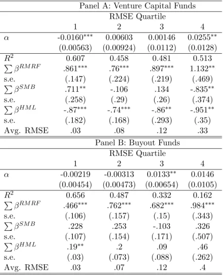
Alternatively, we look at fund performance measured against the Fama and French (1993) three-factor model. Again, we aggregate funds into a value-weighted portfolio and run time-series regressions of quarterly fund returns on current and lagged factor returns. Specifically, we
estimate rit=αi+ 4 X k=0 βikRM RFrRM RFt−k + 4 X k=0 βijSM BrtSM B−k + 4 X k=0 βikHM LrHM Lt−k +νit. (13)
Column (1) (“All”) of Table 3 reports the loading and excess return estimates from the 3-factor model using four lags of each. The remaining columns report estimates of the size-quartile regressions of the same model. Venture capital funds have strong negative loadings on the book-to-market factor, consistent with their investments in small, high-growth opportunities. Larger VC funds in the 3rd and 4th size quartile have larger loadings on this factor. Interestingly, venture capital funds do not load on the small-firm factor. The VC portfolios have statistically insignificant alphas across all size quartiles. Buyout funds, in contrast, exhibit some positive excess returns and have insignificant loadings on the size and book-to-market loadings.
3.4. Idiosyncratic Risk and Returns
Given a market model, we have two approaches to testing whether average returns are related to idiosyncratic risk. The first is a time series method and the second is a cross-sectional estimator motivated by Fama and MacBeth (1973).
3.4.1 Time Series and RMSE
The time-series method first sorts directly on idiosyncratic risk. That is, for each of the 741 buyout and 1040 VC funds with a return history of at least 16 quarters, we estimate equation (13). The square root of the mean squared residuals is then a standard estimate of a fund’s idiosyncratic risk. Funds are then sorted into quartiles based on their idiosyncratic risk, and value-weighted portfolios are formed. These returns are again estimated using (13) where our objects of interest are the estimates ofαi for the four quartiles. In particular, we focus on the estimate of ˆα4−αˆ1
time-series regression is weighted by the number of funds present in that quarter.30
The results are in Table 4. Consistent with the theory, portfolios with higher idiosyncratic risk exhibit higher returns. For VC funds, the lowest quartile has an alpha of -1.6% versus 2.55% for the highest quartile. The latter is statistically larger than the former. Although the estimates are not as stark, the same one-sided test for the buyout sample difference is 1.47% and has a p-value less than 10%.
While these results are consistent with the theory introduced here, there are other possible explanations for these results. For example, our tests hinge on the validity of the assumed linear factor model. If the linear factor model is wrong, then residual risk is correlated with expected returns, because at least some of the relevant covariance is not captured by the factor or factors and thus is lumped into the residual with the true, unpriced idiosyncratic risk.
To investigate this, we also redo the empirical tests using alternative factors. The results are nearly identical if we instead use just Nasdaq stocks to construct the market return, and the results are unchanged if we use a single market factor rather than the three Fama-French factors. We also check for parameter stationarity throughout the sample. When we split the sample, we find no evidence that the linear factor model differs across the two halves. Finally, we address concerns that many of the funds in the the data are younger and cut the sample at the 2002 vintage. Table 5 repeats the exercise above and we find that the fourth quartile alpha (column 4) is still statistically larger than the first quartile (column 1).
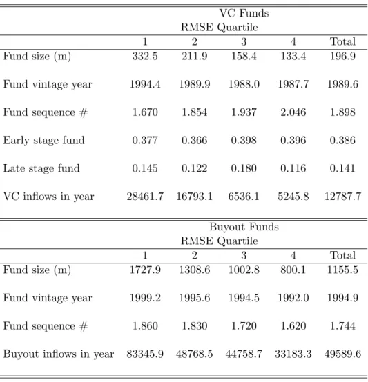
We have thus far shown that portfolios sorted by fund-level RMSE from a 3-factor regression have a strong pattern of excess returns. It is possible that such a correlation is driven by other characteristics of funds within the RMSE quartiles. Table 6 is a first attempt at addressing whether the RMSE portfolios are capturing other observable feature of funds. The merged data has several characteristics of VC funds and a few features of buyouts available. We observe
30
Since we can measure idiosyncratic risk it might seem investors and VCs should contract on it. However, our estimates are measured with error (which is why we form portfolios), thus VCs paid based on measured idiosyncratic risk would still hold considerable idiosyncratic risk and this would not solve the problem. Furthermore, this would give VCs the incentive to manipulate idiosyncratic risk or its measurement, thereby reducing the any value from contracting on it. In any case, investors have little to gain by contracting on idiosyncratic risk, as they are already expecting zero alpha.
the fund vintage, the sequence number, the investment type by stage (for VC) and the total capital inflows into each market by vintage year (e.g. see Gompers and Lerner (2000) for VC). The averages by quartile show that fund vintage, fund size and total capital inflows strongly correlate with RMSE. These relationships motivate a cross-sectional analysis of idiosyncratic risk and returns.
3.4.2 Cross-section and RMSE
We take two approaches to controlling for cross-sectional differences in funds and RMSE. The first follows Ang, Hodrick, Xing, and Zhang (2006) with a refinement of our time series estimator. In that paper, the authors study the pricing of aggregate volatility in the cross-section of returns. They find that the the extreme quintile of portfolios sorted by idiosyncratic volatility have statis-tically different alphas, however, the characteristics of stocks in these buckets differ. For example, in their sample of publicly-traded firms, only 1.9% of the value of stocks are covered in the top quintile of volatility.
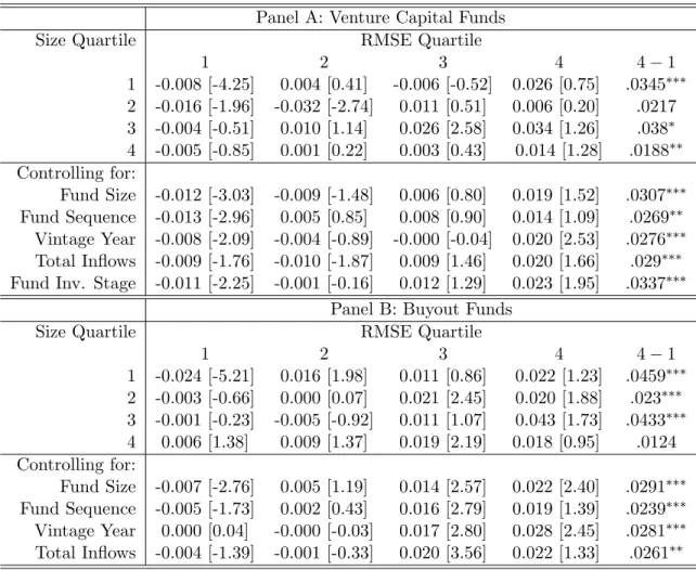
For each RMSE quartile and fund type, we first sort by the observable fund feature such as size. Then within each quartile, we sort again by the RMSE. Thus, within each size or other observable quartile, quartile 4 has the funds with the highest idiosyncratic volatility. Table 7 shows that within each size quartile, the portfolio with the highest RMSE also has the largest alpha estimate. The column “4-1” takes the difference in alpha estimates between the two extreme quartiles and reports the one-sided test p-value.31 These double-sorts quarter the sample for each
α estimate, so we expect significance to fall. All differences are positive, with only quartile 2 of VC funds having a statistically insignificant value. The average of the alphas within the RMSE quartile and across the fund observable allows us to control for size, sequence or other characteristics. The difference of 3.59% for fund size shows that the RMSE relationship with returns cannot be fully explained as a size effect. The second part of each Panel in Table 7
31
Although we often lose statistical significance for the top alphas of the high RMSE quartile in Table 7, the column 4 alpha coefficient is always positive and economically larger in magnitude than the negative coefficient for the smallest RMSE (column 1). Furthermore, the alpha increases from column 1 to 4 in nearly all specifications. This monotonicity says that even if realized returns in VC have been a bit lower than expected, the higher RMSE group has consistently earned a higher return.
presents these cross-section estimates for other observables.
The row “Fund Sequence” creates buckets by the sequence of the firm’s fund: 1, 2, 3 or 4 and greater than 4. Similarly, the “Vintage Year” sort breaks funds into five time periods, starting in 1980. “Total Inflows” uses the total capital invested into entrepreneurial firms or funds raised in LBOs in each vintage year, which then sorts funds into quartiles by this level. Finally, “Fund Investment Stage” buckets VC funds into early stage, late stage and balanced. For each of these additional sorts, the difference in the estimated alphas between the two extreme quartiles of RMSE is statistically significant and positive. We conclude that size, fund sequence, vintage year and capital inflows cannot explain the relationship between average returns and idiosyncratic volatility for VC funds. The smaller set of observables for buyout funds leads to the same conclusion.
This approach goes a long way towards address concerns about omitted variables, however, we cannot jointly control for factors through double-sorts. Our final set of specifications uses the Fama and MacBeth (1973) methodology (used by many authors such as Gompers, Ishii, and Metrick (2003) and Giroud and Mueller (2011)) to test for cross-sectional explanations for the relationship between returns and idiosyncratic risk.32 Consider the following specification of the cross-section of quarterly fund returns:
rit=αt+γXit+ρσi+vit. (14) Here, rit is the quarterly return for fund i in quarter t, Xit contains all the controls discussed above andσi is the fund’s estimated idiosyncratic volatility. Unlike the asset pricing analogue to equation (14), we are not interested in estimating risk premiums and cannot controls for systematic risk estimates as they are too noisy. Instead, we use the Fama and MacBeth (1973) econometric technique of pooled cross-sections to address cross-sectional differences in fund returns. Equation (14) is estimated for each quarter from 1980 to 2011 and the coefficients αt and γ are averaged to obtain the standard Fama-MacBeth estimates and heteroskedasticity-adjusted standard errors with a two-quarter Newey-West lag structure.33
32
The fund data and time series are too short to create a measure of idiosyncratic volatility as in Ferreira and Laux (2007), so we instead use the single measure for each fund.
33
Table 8 reports the results of these regressions for buyout and VC funds. The coefficients of interest are on the variables “Idiosyncratic volatility” and “RMSE quartile.” The latter is defined as the RMSE quartile by vintage year. Columns (1) and (3) show a strong positive correlation between quarterly fund returns and idiosyncratic volatility levels. To capture any non-linearity we introduce controls for quartiles of RMSE. With the excluded category as the lowest quartile, the positive, significant and monotonically increasing coefficients from the remaining quartiles are directly in line with the model predictions. We conclude that the patterns of excess returns and idiosyncratic volatility are not driven by size, fund sequence, vintage, or capital flows.
3.5. Stale NAVs and Idiosyncratic Risk
Another concern is a relationship between the stale NAVs of a VC fund and the measure of idiosyncratic risk. For example, a high-performing fund could mark its portfolio more often, resulting in greater measured idiosyncratic risk and also a large alpha, while poor performing funds could have more stale values and less measured idiosyncratic risk.34 We address this concern in three ways. First, for each VC fund we calculate the fraction of flat NAVs or zero quarterly returns. We find no significant correlation between this variable and a fund’s total return. Next, Table 9 repeats the Fama-MacBeth regressions with an additional control for the fraction of stale values (“% flat NAV”). The inclusion of this variable has no impact on the conclusions. Finally, in an unreported table we split the VC fund sample into two halves based on the fraction of observed zero quarterly returns for all funds with at least 16 quarters of returns. The patterns of positive alpha in the high quartile RMSE and negative alpha in the lowest quartile RMSE remain for both sub-samples. We conclude that heterogeneity in the staleness of a funds NAV cannot explain our main results.
34
It is possible that a fund with significantly more stale NAVs could have a either a better or worse fit to the 3-factor model and thus higher or lower idiosyncratic risk. Therefore the issue must be examined empirically.
4.
Extensions: The Risk of the Portfolio
All of the results in the paper so far hold with any form of contract between the investor and VC, as long as the compensation depends on the payoff of the portfolio. However, we have predicated these results on the assumption that the VC cannot alter the risk of the portfolio. This section considers the validity of that assumption by allowing the VC to maximize his utility by altering portfolio risk. We show that properly structured option contracts (similar to real VC compensation contracts) eliminate the VCs desire to alter the portfolio risk. Thus, relaxing the assumption that the VC cannot alter the portfolio risk would not invalidate our results. Therefore, our theory is robust to an extension that allows the VC to alter the risk of the portfolio.
This section also explains why the standard VC contract pays the VC a fraction of all positive returns on the portfolio. This makes the VC’s payoff like a call option. Since increasing volatility increases the expected payoff from the option, it might seem that this type of contract would encourage excessive risk-taking by the VC. Such incentives could be removed by simply giving the VC an equity contract. Thus, why does the standard contract contain an option? Furthermore, why is the return benchmark above which the VC shares in the profits, usually equal to zero?35 It would seem that the VC should have to at least beat the risk-free rate (if not some higher benchmark) before sharing in the upside. This section shows that the answer to both questions is the same; the VC contract must neither encourage nor discourage the VC to spend time to alter the risk of the portfolio. The diversified investor does not care about the risk in any small part of his portfolio, so the investor wants the VC to increase the mean, not change the amount of idiosyncratic risk. We show that an equity contract encourages diversification, and an out-of-the-(expected)-money option contract encourages excessive risk taking. Thus, an option with a low strike price (i.e. no hurdle rate) encourages effort while providing little benefit to changes in risk.
To consider the question of risk we examine a very general formulation of our model with
N >1 and VC utility function over wealth,u(w).We assume that the VC is risk-averse but likes wealth so that u0(w) >0 and u00(w) <0 and that the portfolio is sufficiently good that more of
35
see Fleischer, Victor, “The Missing Preferred Return” (February 22, 2005). UCLA School of Law, Law-Econ Research Paper No. 05-8