Private Intergenerational Transfers and Their Ability to Alleviate the Fiscal Burden of Ageing
(Preliminary draft: May 2007) By
Dr Hayat Khan
Department of Economics and Finance, School of Business, La Trobe University,
Bundoora, VIC 3086.
Email: h.khan@latrobe.edu.au Ph: +61 3 9479 3536 Fax: +61 3 9479 1654
Abstract: The ratio of retirees to workers in developed countries is expected to increase sharply in the next few decades. In the presence of unfunded income support policies, this increase in old age dependency is expected to increase the future fiscal burden which is seen as a threat to living standards. This paper quantifies the ability of private intergenerational transfers to alleviate the future fiscal burden of ageing. This is done through developing an extended dynamic overlapping generations simulation model with realistic demographics. Calculation based on steady state simulations suggests that a bequest to GDP ratio of 1% offsets about 33.3 % of the fiscal burden over the lifecycle when measured as a % of simple labour income and 8.9% of the fiscal burden when measured as % of the full income. The model is calibrated for Australia under small open economy assumption such that the optimal solution mimic important cross sectional and time series fundamentals of the Australian Economy. Intergenerational accounting suggests that the empirically plausible intergenerational transfers are strong enough to offset most of the tax burden (81 to 91%) when measured as % of simple labour income and up to ¼ of the burden when fiscal burden is measured as % of full income. In the endogenous labour supply case, 81 to 91 percent of the fiscal burden of ageing will be alleviated by inheritances in the base case. Due to the calibration strategy adopted, the paper analytically demonstrates that results of the simulations are robust to the introduction of lifetime uncertainty in the model where people discount the future by a rate of time preference and by a survival probability irrespective of whether there are perfect annuity markets or no annuity markets at all.
1. Introduction
Most of the developed and some developing countries are undergoing or projected to experience a significant change in their demographic structure. Population projections under alternative assumptions about fertility, mortality and immigration reveal that the proportion of retired population, those 65 and above as percentage of total population, will grow sharply. For example in Australia, alternative population projection reveal that the ratio of retirees to total population will increase by more than 10 percentage point, nearly double the current level, in the next few decades.
With unfunded income support policies in place, this ageing of the population is projected to significantly increase future fiscal burden of the ageing population which is seen as a threat to future living standards. Because saving is a means to redistribute living standards over time, researchers have debated the optimal response of national saving to offset adverse effects of the fiscal burden due to ageing. There has been a difference of opinion as to whether the optimal response to an ageing population is an increase in national saving or a decrease. Some have called for a significant increase in the level of saving (Guest and McDonald (2001), OECD (1996), Fitzgerald (1993),), whereas others have proposed the opposite (Auerbach, Kotlikoff, Hagemann and Nicoleti (1989), Cutler, Poterba, Sheiner, and Summers (1990), Auerbach, Kotlikoff and Cia (1990), Elmendorf and Sheiner (1990) and Miles (1999)).
Raffelhuschen (1999) and Kotlikoff and Raffelhuschen (1999) generational accounting studies found that 19 out of the 22 countries investigated exhibit a fiscal imbalance to the disadvantage of future generations. These accountings, like many others, focus on public intergenerational transfers (such as social security, health care and old-age care) as pointed out by Lueth (2003) and ignore the role played by private intergenerational transfers. Lueth (2003) uses an overlapping generations model to investigate the potential of private intergenerational transfers to alleviate the fiscal burden of population ageing. The fiscal burden is modelled as a PAYG pension scheme. Lueth argues that due to decline in the number of bequestees, inheritances are expected to increase. The parameter that quantifies the intensity of bequests is set such that bequest turns out to be 5.8% of GDP which corresponds to the German circumstances. This increase is however insufficient to make up for the fiscal burden induced by demographic change.
Lueth (2003) however uses a two period overlapping generations model which does not capture true structure of an economy. Theoretical properties of the model do not carry well to a model with multiple overlapping generations. Individuals in the Lueth’s model expect to live for two periods (working in the first period and retired in the second) where every body lives through the first period and a fraction of them die prematurely in the beginning of the second period. Short lived individuals therefore leave accidental bequests only at the end of the one period working life.
This paper however argues, and simulations confirm it later, that most of the accidental bequests are left by the retired population. Since the issue is one of quantification, its important to bring some more realism into the model. Khan (2006) simulated earlier version of the extended model where labour supply was assumed to
be exogenous to study the impact population ageing on living standards and the optimal response of national saving, investment and current balance to prospective ageing in Australia. The paper allows labour supply to be endogenously determined. On the theoretical sides, Khan (2006) modelled four aspects of a demographically changing economy. These aspects were (i) young and old-age dependencies (the proportion of retired pensioners and young dependents to the working population), (ii) the changing productivity of individuals as they age, (iii) the age-varying nature of consumption demands (following Cutler et al (1990) and Guest and McDonald (2001)), and (iv) in an economy with altruistic agents or in case of accidental premature deaths, the number of bequests recipients (inheritance related support ratio). This paper retains all those modifications and in the context of endogenous labour supply models variation in leisure demands by age in the same manner as consumption demand.
Khan (2006) extended the Miles (1999) model which builds up on AK(1987) to model the aforementioned features. The extensions made were (i) accounting for children, (ii) extended planning horizon, and (iii) allowing individuals to die anywhere along the lifecycle as in actual data (and leave bequests, intentionally or unintentionally). Like Khan (2006), this paper uses actual primary data on demographics organized by age, historical and projected. In the actual data on demographics the maximum age of an individual may exceed 100. A representative individual in the model is therefore assumed to live up to a maximum of 101 years, 17 as young non-working child (determined through simulations), 48 as working adult and 36 as retired pensioner. Like the actual data on demographics, the individual may die anywhere along the lifecycle. In AK (1987) individuals live till the age of 75 whereas in Miles (1999) they live for 60 adult years.
On the applied side, an important feature of the paper, like Khan (2006), is that the extended model is parameterized such that the optimal response of the simulations emulates important cross-sectional (1997) and time series (1990 to 2003) fundamentals of the Australian economy (see the section on simulations for detail)1.
Table 1: The Extent of Ageing under Alternative Assumptions on Fertility The population of people aged 65 and above as percentage of the total
population Projectio n Total Fertility Rate (TFR) 2003 2032 2049 Base Case 1.75 from 1999 onwards 12.43 20.08 22.2 TFR1.65 declines from 1.75 to 1.65 in 2004 12.5 20.5 23.06 TFR1.3 declines from 1.75 to 1.30 in 2009 12.53 20.95 26.13 1
The word “optimal” here is not used in the context of social planner like GM (2001). It refers to the fact that individuals in the economy make optimal choices given certain demographic and institutional structure.
Note: (i) For all these projections, life expectancy increases by 0.4 years every five years and annual net migration is 0.54 % of the total population. (ii) The first year of projection is 1999
The rest of the paper is organized in the flowing manner. Section-2 gives a detailed description, solution and interpretation of the model. Section 3 outline general equilibrium solution of the model and describes the algorithm used to solve the model in general equilibrium. Section 4 simulates the model for the Australian Economy. This section outlines the way different preference and technology parameters are fixed and report the results of the simulations. Section 5 discuses whether the bequests generated by the model are joy-of-giving or accidental. Section 6 compare the base case model of the paper with alternative specification where lifetime uncertainty is explicitly model. Finally, section 7 concludes the paper.
2. The Model
The model comprises four sectors; a household sector, a single production sector, a government sector, and an international trade sector. Whereas households maximize discounted sum of their lifetime utility subject to lifetime budget constraint; production sector is assumed to maximize its profits. Government is assumed to run balance budget and is committed to a pure pay-as-you-go (PAYG) pension scheme. International trade sector allows locals and foreigners to hold each other’s assets as well as trade in output. Jointly these four sectors determine the economy’s dynamic equilibrium path.
The model in this paper is a multi-period over lapping generations model where a representative individual is assumed to live for 101 years (101 is the maximum age in data on demographics) and allow for (i) young and old age dependencies, (ii) a hump-shape age-productivity profile, (iii) age-varying consumption and leisure demands, and (iii) intentional and unintentional intergenerational transfers.
To model the young age dependency, it is assumed that individuals do not work when they are children, 0 to TC (=16 which is determined through simulations) years of age, and their consumption is chosen and financed by their parents. On entering the labour market in the age of 18, individuals work full time till they retire at the age of 65. To model old-age dependency, it is assumed that the retired individuals, aged 65 and above, receive certain amount of state pension that is financed through tax collected from working population in that period (PAYG system).
The age productivity relationship is modelled using Miles (1999) formula where log of the age-specific labour productivity is given by:
2
0.05age- 0.0006age (2.1)
In the absence of time related rise in productivity, market value of the endowment peaks at the age of 42. With a total factor productivity growth rate of 1%, the actual for Australia (GM 2001), the time related rise in labour productivity (equal to the average long run rise in output per head) turns out to be 1.5%. The market value of the endowment with the 1.5% time related rise in labour productivity peaks at the age of 54 (see figure 3 below).
Following CPSS (1990), Guest and McDonald (2001) and Khan (2006), individuals are assumed to have age-varying consumption demands. Technically speaking, this means that a unit of consumption is not as efficient in delivering satisfaction to an old person as it is in delivering satisfaction to a young. The idea is extended to leisure as well. It is assumed that leisure demand of individuals change with age as well and a unit of leisure is not as efficient in delivering satisfaction to an old person as it is to a young. This is captured through making utility a function of consumption and leisure demands.
The model outlined in this paper allows people to leave bequests to later generations. By nature, these bequests are either optimally chosen (intentional) along with lifetime consumption and leisure or accidental (unintentional). Intentional bequests are a manifestation of joy of giving which is also referred to as bequests as consumption behaviour, whereas unintentional bequests are caused by premature deaths referred to as accidental bequests2.
The idea of accidental bequests is motivated by the fact that, in historical and projected data on demographics, not all individuals survive to the fully anticipated lifetime. Those who die prematurely (referred to as accidental deaths) may leave behind some wealth, negative or positive, referred to as accidental bequests. It is assumed that every agent in the economy knows with certainty the number of accidental deaths in each age-group and the amount of wealth they leave behind, negative or positive. Although, individuals know with certainty how many of the agents in each age group will die, they however are not sure about who exactly those agents will be and, therefore, in planning lifetime consumption totally ignore, for convenience, the possibility of their own premature deaths. Individuals therefore plan for T adult periods, where T(=100-TC) is the maximum possible planning horizon on entering the labour force.
In the base case model we ignore explicit incorporation of heterogeneity by planning horizon and lifetime uncertainty. Later in the paper, I discuss the implication of such modification in the model. It is shown that that, under conditions, acknowledging the existence of individuals with heterogeneous planning horizon will not change results of the model. Similarly, it is analytically shown that due to the calibration/simulation strategy adopted in this paper incorporating lifetime uncertainty in the model will give exactly the same result as the base case model irrespective of whether or not there are perfect or imperfect annuity markets. This is because the calibration/simulation strategy automatically accounts for lifetime uncertainty.
Let us now explain each sector of the model in detail. 2.1 Household Sector:
2
Theoretically speaking, part of these unintentional accidental bequests may be intentional joy-of-giving bequests planed to be transferred at the end of life. However, what makes it accidental is the fact that individuals were planning to transfer it at the end of the full planning horizon but due to their
This section describes behaviour of the households; their preferences, budget constraint, and their decision making processes.
2.1.1 Household’s Preferences
Households in this model choose their lifetime consumption and leisure along with consumption of their children and joy-of-giving bequests on the basis of their lifetime resources. It is assumed that individuals derive utility from their own consumption as well as spending on their children, leisure and joy-of-giving bequests. They optimally choose these values subject to their lifetime budget constraint.
I assume that in the beginning of lifecycle individuals do not work from 0 to TC (TC+1 periods); enter labour force after TC+1 years and work till they retire when they turn 65 (TC+1 to 64 for 64-TC years); and remain as retired state pensioners till they live to a maximum of 101 years from 65 to 100 (36 years).
Following Miles (1999), for the sake of convenience, through out this paper I index generations by the year they enter the labour force. In general i represents the time a particular generation, referred to as generation i, enters its adulthood or joins the labour force. τ represents time. Thus at a given point in time, τ, a representative agent in generation i is (TC+1)+(τ-i)+1 years of age with (TC+1) years spent as nonworking child and (τ-i)+1 as working adult. For a quick reference, this is depicted in Figure 1.
Figure 1: Planning horizon, generations indexing and their age
In light of the above discussion, the lifetime utility function of a representative agent in a generation i is assumed to take the following functional form3,
(
)
( )(
)
( )(
)
( ) w i+ T -1 i+ T-1 , , , , i 1 , =i , , =i , 1 1 = , 1 1 1 c c i i i i i i c i b i i c T i i i i c l n c n b V u u u p g x n τ τ τ τ τ τ τ τ τ τ τ τ ϕ ω ρ − ρ − ρ − − + + + + + ∑
∑
(2.2)where T(=100-TC) is length of the planning horizon on entering the labour force and Tw(=64-TC) is the number of periods an individual stays in the labour force.
(
)
( )
,( )
, , , 1 1 1 1 1 1 1 1 1 1 1 1 , , , , 1 , i i i i c l p g i i i i c l p g u τ τ τ τ ξ ξ τ τ τ τ η γ η η − − − − − − − + = is the instantaneous utility function
of a representative agent, where 0≤ ≤li,τ 1 is proportion of the available time allocated to work,
(
1−li,τ)
is the proportion of time allocated to leisure; ci,τ is the consumption of a representative agent in generation i at time τ, pi,τ the age specific consumption efficiency weights of the agent when in (τ-i+1)th year of his/her working life (the higher, the least efficient), i,i, c p τ τ is therefore consumption measured in efficiency units also referred to as consumption per consumption units and living standards; gi,τ, an equivalent of pi,τ for leisure, is referred to as leisure efficiency weights of the agent when in (τ-i+1)th year of his/her working life
( )
, , 1 i i l g τ τ −is leisure measured in efficiency units or leisure per leisure unit;
, , c i c c i c u x τ τ
is the utility a parent derives from spending on her ,
c i nτ children at time τ defined as
( )
1 1 , , , 1 , , 1 1 c c i i i c c c i i c c u x x ξ τ τ τ ξ τ − = − , where , c i cτ consumption of his/her , c i nτ children (population of children divided by working population), and ,c i
xτ the number of children measured in consumption units (weighted by their consumption efficiency weights)4; and ,
i i b i b u n
the utility derived from bequeathing expressed as
( )
1 1 , 1 1 1 i i i b i i b b u n n ξ ξ − = − , where n the number of bequestees per donor (total i number of working population relative to old generation) and bi the size of
bequest made by a representative agent in generation i at the end of his/her life to later generations (the working population only).
1 i τ
ϕ + − is the weight assigned to the utility parents derive from spending on their children when they (parents) are in
(
τ − +i 1)
’th year of their working life. ρ is the rate of time preference, ξ the intertemporal elasticity of substitution of consumption as well as leisure, γ quantifies the preference of leisure over consumption, η determines the substitutability of consumption and leisure respectively, and ω the weight placed on joy-of-giving bequest.2.1.2 Household’s Budget Constraint:
The household’s lifetime resources come from three sources; labour income, state pension, and shares in bequest from previous generations, generations that die when the agent is part of the labour force. The budget constraint for a representative agent in generation i is
4 , , 0 c T c j i i j nτ nτ = =
∑
and , , , 0 c T c j j i i i j xτ p nτ τ ==
∑
where TC is the age of the eldest child and ,j i
pτ the consumption
( ) ( ) ( ) ( ) ( )( ) ( ) ( ) ( ) ( ) ( ) ( ) τ τ τ τ τ τ τ τ τ τ τ τ τ τ τ τ τ τ τ + − + + − + − + − − − − − − − = = = + = = − + + + − − = + + + + + +
∑
∑
∑
∑
∑
1 1 1 1 , , , , , , , ( 1) 1 1 1 1 1 1 1 w w w w i T i T a i T i T i T c i t i i i i i i i i i i i i T i i i T i i w l h b b PN c c b r r r r r r iV is the notional stock of wealth at the end of life available for enjoyment in the form of consumption, leisure, spending on children and bequest. In the literature, this is referred to as “full-income”.
Important aspects of this constraint are outlined as follows.
i. Labour Income: hi,τ the age-specific endowment of effective units of labour available to each member of generation i at timeτ (determined by the Miles (1999) formula stated above), w is the real wage rate that grows at the t rate of total factor productivity and li,τthe proportion of time spent working.
, ,
i i
w l hτ τ τ is therefore the labour income of a representative agent in generation i at time τ . τt is the PAYG tax rate. wτ(1−τt)l hi,τ i,τ is therefore the
corresponding disposable labour income. The first term on left hand side of the budget constraint is present value of the disposable labour income over the working life.
ii. State Pension: PNi,τ is the state pension received by a representative
agent in generation i in period
τ
. This income is positive only after agents retire, in old age, otherwise zero. The third on the left hand side of the budget constraint is therefore present value of pension stream received by the representative agent over retirement.Pension benefits, PNi,τ, in the model are calculated at an exogenously given
replacement rate. Replacement rate, rept, is the average pension as proportion of
average labour income and, thus, can be expressed as
( ) ( ) ( ) ( ) τ τ τ τ τ τ τ τ τ τ τ τ τ τ − − = − − − = − − − = − − = ∑ ∑ = = ∑ ∑ 1 , , 1 , 1 , , 1 , average pension
average labour income
T i i i Tw T i i Tw Tw i i i Tw i i N PN N t N y N rep (2.3)
Recall that government is committed to PAYG pension scheme and runs a balanced budget. The government budget constraint can be written as
iii. PAYG tax rate and old age dependency: tτ is the tax rate levied on any labour income at time τ. Like Miles (1999), for a given replacement rate the tax rate on labour income in each period ( tτ) is set so as to balance aggregate pensions paid against total tax receipts (PAYG) i.e.
( ) ( ) 1 1 , , , , w w T T i i i i i i T t N y N P N τ τ τ τ τ τ τ τ τ − − − − = = − =
∑
∑
orwhere the left hand side is the tax revenue collected from imposing tax at the rate tτ on labour income of the working population, and the right side is the aggregate pension paid to the retired individuals.
From equation (2.3) and (2.4)
( ) ( ) ( ) ( ) τ τ τ τ τ τ τ τ − − = − − − = = =
∑
∑
1 , 1 , retired population replacement rate working population w w T i i T T i i N rep N t (2.5)Thus, a one percent increase in the proportion of retired population relative to the working population will increase PAYG tax rate by the replacement rate. Since working population has to finance the pension paid to retired population, this PAYG tax rate captures the old-age dependency aspect of ageing.
Note that the equilibrium rate of PAYG tax rate is independent of labour income (hence labour supply). Thus, tax rates will remain the same irrespective of whether labour supply is exogenous or endogenous. The intuition behind this result is this. Whereas, on one hand, an endogenous decline in labour supply decreases average labour income which puts upwards pressure on the PAYG tax rates, on the other hand, the decline in average labour income reduces state pension at a given replacement rate (equation (2.3)) which puts downward pressure on the PAYG tax rate. In equilibrium these two effects cancel each other out.
iv. Share in bequests received from previous generations: Because the model assumes that in each period one generation dies and another newly born takes its place and that some agents in each generation die prematurely, in each period individuals receive bequests from those died in the last period of their life or prematurely. The paper assumes that individuals are entitled to receive bequests only when they are in the working force and that these bequests are equally shared by the working population.
, i
bτ denotes the share of bequests received by a representative agent in generation i at time τ from agents who died in the last period, bequeathed as joy of giving, and bia,τ the share in bequests from agents who died prematurely as accidental bequests. The superscript “a” stands for accidental.
I assume that these bequests are made at the end of each period and are received by the beneficiaries in start of the next period5. Thus, i, (1 ) 1
b b r n τ τ τ − = + where bτ−1
is the bequest left by a representative agent in generation τ-T dying in period τ-1, and nτis the number of working children in period τ-1 alive in period τ
6 .
5
Think of this as a contract written in favour of an individual in the working population entitling him/her to receive his/her share after the older generation passes away.
6
As the bequests made are received with a year lag, they earn marginal product net of depreciation that in equilibrium is equal to interest rate. Hence, the per-person bequest is multiplied by (1+r).
Similarly, bia,τ is the share in bequests received from those died prematurely. This value is obtained by summing the products of the number of agents in different age groups who die in each period and the wealth each one of them leaves behind, and dividing it by the number of agents sharing it. i.e.
( )
(
,)
, 2 , , 1 1 w i i a i T i i i T r D e a th s w b N τ τ τ τ τ τ = − + = + =∑
∑
(2.6)Later in production sector of the model I assume that all of the household wealth in each period is used to build up domestic capital or acquire foreign assets, these bequest shares therefore are in the form of ownership of assets. Individuals can trade these assets in local or international markets if they decide to consume, all or part of, it.
The second term on the left hand side is therefore present value of the shares in bequest, joy of giving or accidental, received by the representative agent over the lifecycle.
v. Young-age (childhood) dependency:
As mentioned earlier, individuals spend cic,τ , which is optimally chosen, dollars on the consumption of their c,
i
nτ children. The model considers children as responsibility of the working population in the society and thus calculates c,
i
nτ as ratio of the population of children in a particular period to the size of the working population in that period. Individuals therefore spend on children through out their working life. This approach is in line with the fact that in some countries, like Australia, government provides for some of the consumption of the children which is financed through taxation. Here I do not involve government and let the parents choose the spending optimally. Part of the spending not financed through government taxation can be thought of as inter-vivos transfers to their children.
This is unlike AK (1987) where children are born when parents are 21 years of age. Parents optimally choose consumption of their children until their children turn 21. That is when their parents are 40. Parents do not spend on their children when they are older than 40 years. Another difference is that children in the model in this paper don’t work whereas in AK (1987), children work as well. The last two terms on the left side of the budget constraint represent present value of the individual’s own and his children’s lifetime consumption. Notice that individuals take care of their children only when they are working, implying that children are the responsibility of the working population only.
For convenience, let us reproduce the budget constraint above as
( ) ( )( ) ( ) ( ) ( ) ( ) ( ) ( ) ( ) τ τ τ τ τ τ τ τ τ τ τ τ + − + − + − − − − − − = = = − − − − − = + + + +
∑
∑
∑
+ 1 1 1 , , , , ( 1) ( 1) 1 1 1 1 1 1 1 w w i T i T i T c i i i i i i i i i T T i i i w t l h c c V b r r r r r (2.7) ( )[( ) ( )] ( ) ( ) ( )[( ) ( )][ ] ( )[( ) ( )] ( ) τ τ τ τ τ τ τ τ τ τ τ τ + − + + − − − − − − − − − − = =+ =+ =∑
+ − +∑
+ + +∑
+ 1 1 1 1 1 , , , , 1 1 1 1 1 w w w i T i T i T T i T i a T i i i i i i i i i T V r w t h r b b r PNi
V is the notional stock of wealth at the end of life available for enjoyment in the form of consumption, leisure, spending on children and bequest. In the literature, this is referred to as “full-income”. The second term is present value of the leisure consumed over the lifetime. The remaining terms bear the same interpretation as before.
2.1.3.
Solution of the Model:Formally, households maximize (2.2) subject to (2.7) thereby choosing
{ }
i, i (T 1)i c τ τ+ − = ,
{ }
( 1) , w i T i i lτ τ + − = ,{ }
( 1) , w i T c i i cτ τ + −= and bi. The first order conditions result in the following
key relationships between consumption, leisure, spending on children, and bequests. For τ = i,...,i+(Tw-1)
(
)
(
)
, 1 , , , , 1 1 i i i i i g l c w t h p η τ τ τ τ τ τ τ η γ − − = − (2.8) ( ) η ξ ξ η ξ τ τ τ τ τ τ τ ϕ − − − = 1 1 , , , , , , 1 c i c c i i i i i x c n c p M (2.9) For τ = i,...,i+(T-1),( )
( ) [ ](
)
( ) [ ] ξ η ξ τ ξ ξ η τ τ τ ρ ω − − − − − − + = + 1 ( ) 1 1 , , , 1 1 1 T i i i i i i b c p M r n (2.10) where{
[ ( ) ](
,)
( )}
( ) , , 1 1 1 , 1 1 i w i i i T g i p i M w t h τ τ τ η η η τ τ τ τ γ − − + − = = + − and { } ( ) τ τ + − = + = , 1 1 w i i T i T M .Equations (2.8) and (2.10) together with the budget constraint gives the optimal joy of giving bequests, bi, which is
ξ ω = ∇ i i i i n b V (2.11)
Similarly, we can derive
( ) [ ]
( )
( ) [ ] τ ξ ξ ξ τ τ τ η η ρ − − − − − − + + = ∇ 1 ( ) 1 1 , , , 1 1 T i i i i i i p M r c V (2.12) ( ) ( ) ( )( )
( ) [ ] τ ξ ξ ξ ξ τ τ τ ρ ϕ − − − − + + = ∇ 1 ( ) 1 , , , 1 1 T i c c i i c i i i n x r c V (2.13)Adding (2.12) and (2.13) we get
( ) [ ] ( ) ( ) ( )
(
)
( ) [ ] τ ξ ξ ξ ξ ξ ξ τ τ τ τ τ τ η η ϕ ρ − − − − − − − + + + + = ∇ 1 ( ) 1 1 1 , , , , , , 1 1 T i c c i i i i c i i i i p M n x r c c V (2.14) where ( )( ) ([ ) ( )]( )[( ) ] ( ) ( ) ( ) ( )( ) ( ) ξ ξ ξ ξ τ ξ ξ ξ τ ξ τ τ τ τ τ τ η ω ρ ϕ − + − − − − − − − − − − − = ∇ = + + + + ∑
1 1 1 1 1 1 ( ) 1 1 , , , , 1 1 i T T i T i c c i i i i i i i n r p M n xi
V is the notional stock of full-wealth, or full lifetime-income, at the end of life available for consumption in the form of own consumption, leisure, spending on children, and bequests over the lifecycle. Following Khan (2006) we can show that the denominator of the right hand side of equations (2.15) to (2.16), ∇i, measure of
the lifecycle family over the planning horizon (referred to as utility worth of the effective lifecycle family) and the numerator in equation (2.14) is argued to be size of the family at a given point in time over the lifecycle (referred to as utility worth of the size of the instantaneous family).
To show this let us first give an interpretation to Mi,τ. Let η =ξ =1, pi,τ =gi,τ =1 ∀
τs, r=ρ=0, and γ=1. Imposing these restrictions, the value of Mi,τ before retirement is
equal to 2. The imposed restrictions make leisure and consumption equally desirable and since individuals consume both at a given point in time, the effective size of the representative agent in terms of consumption goods equals 2. I refer to this as effective size of the representative agent7.
Imposing these restrictions together with ϕ=ω=1 reduces equations (2.11) to (2.14) and rearranging we get
[ ] ( ) [ ] ( ) τ τ τ + − + − = = + = +
∑
+ +∑
1 1 , 2 1 W W i i i T i T i c i i i i T b n V n n [ ] ( ) [ ] ( ) τ τ τ τ + − + − = = + = +∑
+ +∑
, 1 1 , 1 2 1 W W i i T i T i c i i i i T c V n n [ ] ( ) [ ] ( ) τ τ τ τ τ + − + − = = + = +∑
+ +∑
, , 1 1 , 2 1 W W c c i i i T i T i c i i i i T c n V n n [ ] [ ] ( ) [ ] ( ) τ τ τ τ τ τ + − + − = =+ + + = +∑
+ +∑
, , , 1 1 , 1 2 1 W W c c i i i i T i T i c i i i i T c c n V n nConsider denominator in the above reduced equations,
[ ] ( ) [ ] ( ) τ τ τ + − + − = = + +
∑
+ +∑
1 1 , 2 1 W W i T i T c i i i i Tn n . The first term is the number of bequestees per donor. The second and third term is the effective size of the household during the working period and retirement respectively. The whole term is therefore effective size of the family over the lifecycle, referred to as effective size of the lifecycle family.
Now consider numerators in the above equations. ni is the number of bequestees
per donor at the end of life. Thus, the optimal value of bequests relative to the full lifetime-income available for enjoyment is determined by the number of bequestees relative to the effective lifecycle family. Similarly, consumption of the
7
It turns out that under similar restriction n number of choice variables in the utility function would give an effective size of the representative agent equal to n.
representative agent relative to the full lifetime income at a given point in time over the lifecycle is determined by size of the agent (=1) relative to the effective size of the lifecycle family, and that of children by their number (nic,τ) relative to
the effective size of the lifecycle family. From perspective of a family as a whole, the consumption enjoyed by the family at a given point in time (ci,τ +cci,τ) relative
to the full lifetime income is determined by size of the instantaneous family (1+nci,τ) relative to the effective size of the lifecycle family.
Thus consumption of an agent (family) at a given point in time is determined by utility worth of the size of the agent (family) at the point relative to the utility worth of the effective size of the lifecycle family.
2.2 Production Sector:
The model is characterized by a single production sector behaving competitively. The sector is assumed to use capital and labour as inputs subject to Cobb-Douglas production function. Capital is assumed to be homogeneous and depreciating at a rate equal toδ 8. The production function is given by
α α
τ = τ τ 1τ−
Q A K L (2.17)
Qτ is aggregate output of the economy,Lτ is the aggregate employment level, and
Kτ the aggregate capital stock used in domestic production. Competitive nature of the production sector requires all factors of production to be paid according to their marginal productivity. Aτ is technology that grows at the rate
“a”(Aτ =A0(1+a)τ). Thus α τ τ τ α δ − − = − (1 ) K r A L (2.18) τ α τ τ τ α = (1− ) K w A L (2.19)
By the overlapping generation nature of the model, aggregate employment is the sum of labour hours supplied by the working population in the economy i.e.
( ) ( ) , , , , 1 1 w w i i i i i T i T L L N l h τ τ τ τ τ τ τ τ τ = − − = − − =
∑
=∑
(2.20)Domestic capital stock comes from aggregate household wealth (W ) net of foreign t assets holdings (F ) .So, t Kτ =Wτ−1−Fτ, where the total wealth is the sum of
individuals’ wealth in the economy, given by
( ) ( ) , , , 1 1 w w i i i T T W W N w τ τ τ τ τ τ τ− − τ− − =
∑
=∑
(2.21) ( ) τ ( ) τ = − τ τ + τ + τ + , − τ − τ + + τ− , 1 , a, , i , c, 1 , 1 i i i i i i i w t y b b PN c c r w (2.22)2.3 International Trade Sector:
The international trade sector allows trade in assets and trade in final goods. Thus at any point in time a household’s wealth is in the form of domestic assets (Kτ) and,
or, foreign assets (Fτ), net foreign assets in broad terms. Because, return on assets
8
across countries is the same and that they are perfectly mobile and equally tradeable, domestic and foreign assets are perfect substitutes.
Apart from trade in assets, the model acknowledges trade in final output as well. The intuition is that simply allowing for capital inflow or outflow induced by interest rate differential doesn’t necessarily imply a production level matching consumption demands in that period. Assuming that the single production sector produce consumption goods as well as domestic capital goods, the difference between total production (Qτ) and the sum of consumption and investment in
domestic capital equals net-export i.e.
NXτ =Qτ −Cτ −Iτ (2.23)
2.4 Government Sector:
In the present version of the model government plays a very limited role. Government simply supplies a government pension to people in the old period of their lives. Tax is collected to balance the government budget in each period. Thus the government pension is a PAYG scheme.
3. General Equilibrium Solution of the Model:
There are three issues that need attention in obtaining a general equilibrium solution to the model: the starting-values problem, calculating the optimal values of accidental bequests, and the end-values problem. These issues are addressed in the same manner as discussed in Khan (2006).
Although general equilibrium properties of the model with endogenous labour supply are similar to those of a model with exogenous labour supply (which was described in Khan (2006)), the algorithm described in Khan (2006) needs a slight modification to get a general equilibrium solution to the extended model. The modified algorithm is briefly described below.
Previously, in Khan (2006), labour income was exogenously given, so PAYG pension was calculated exogenously at a given replacement rate. However, with endogenous labour supply this no longer holds. For labour income equals w l hτi,τ i,τ, I can either
make a guess at li,τ ∀ i and τ, the proportion of time allocated to paid work (both wt
and hi t, )
9
, calculate the PAYG pension at the exogenously given replacement rate, revise the guesses until it matches the actuals; or, guess the PAYG pension and revise it until they match the actual ones. The second option is more straight forward and easy to implement than the first. So, I proceed with that one.
A guess at the PAYG pension and accidental bequests is used to calculate optimal consumption, spending on children, the proportion of time spent working, optimal joy-of-giving bequests and the share received by each bequestee, and the saving and wealth profile of each representative agent in each generation. The resulting wealth profiles over the lifecycle are used to calculate the share in accidental bequests received by each representative agent, which is obtained by multiplying the number of
9 t
w has time related productivity component, At, and needs a starting value. Here I assume the
accidental deaths in each age group by their respective wealth and dividing by the number of bequestees.
Similarly, after getting estimates of the proportion of total available time allocated to work, I calculate the income from labour and calculate the actual PAYG pension at the given replacement rate. Guesses at the PAYG pension and accidental bequests are updated until they match the actuals.
As the model is that of a small open economy with perfect capital mobility, r is fixed at the world rate. Using equation (2.18) I can calculate the optimal value of capital
stock, τ α τ τ α δ − = + 1 1 A K L
r , and investment in the economy. Also, I can calculate lending (borrowing from) abroad using Fτ =Wτ−1−Kτ and optimal current account
balance as CABτ =Fτ −Fτ−1. A series of optimal national saving is obtained by
adding current account balance with investment. This process is depicted in Figure 4.
4. The Simulations:
4.1 Fixing Values of the Parameters and Some Exogenous Variables
In general, the model is calibrated such that optimal response of the simulation mimics important cross-section (1997) and time series (1990 to 2003) fundamentals of the Australian economy. Some of the parameters are exogenously set and other determined such that the following targets, which are representative of the cross-section and time series fundamentals, are achieved,
(i) the optimal distribution of consumption by age in 1997 closely follow the actual for Australia in that period,
(ii) the optimal value of capital output ratio approximates the actual for Australia in period 1990 to 2003, and
(iii) aggregate bequests as percentage of GDP in year 2000 stay close to the empirical estimates for the US economy,
(iv) the optimal value of GDP in year 2000 equals the actual for Australia, (v) optimal national saving, investment, and current account balance as
percentage of GDP during 1990 to 2003 mimic the actual for Australia, (vi) the optimal gap between gross national saving and net national saving
emulates the actual for Australia during 1990 to 2003.
(vii) the average number of hours worked per week in year 2000 equals 40. The consumption efficiency weights over the lifecycle (pi,τ) and production
possibilities (hi,0), before 1997, are fixed such that the optimal distribution of
consumption by age in 1997 approximates the actual distribution of consumption by age in that period10. This is done in the base case model where labour supply is
10
Initially, at givenhi,0, simulations were carried out to fix pi,τ’s aiming at getting the
exogenous. Figure 5 plots the actual and resulted optimal distribution of consumption by age in 1997. Figure 6 plots the consumption efficiency weights associated with the age distribution of consumption by age (as depicted in Figure 5). Leisure units per person are set equal to the consumption units per person. i.e.pi,τ=gi,τ.
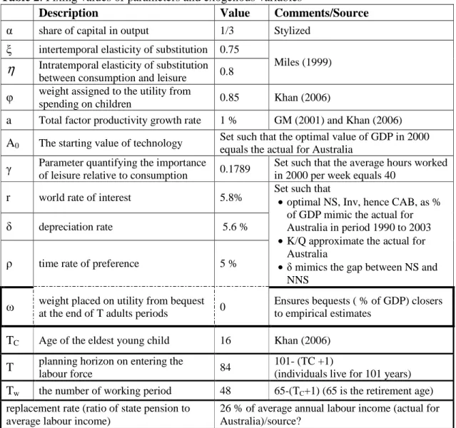
Following Miles (1999), the intertemporal elasticity of substitution, ξ, is set at 0.75 and the intratemporal elasticity of substitution between consumption and leisure,
η
, is fixed at 0.8. Following Khan (2006), TC is set equal to 16, and the weight placed on utility from spending on children (ϕ) fixed at 0.85. Both Tc and ϕ were determined through simulations by Khan (2006).The weight placed on utility from bequests (ω) is set such that aggregate bequests as a percentage of GDP stays as close to similar empirical estimates in the US, since there is no reasonable range for Australia so far, which ranges from 1.5 to 2.65 % of GDP as estimated by Lutz 2002.
ω
determines the level and evolution of an individual’s wealth over the lifecycle. Asω
goes down, wealth at each point in time for all generations decreases and, for exogenously given accidental deaths, the aggregate wealth transferred to bequestees goes down. Since the model tend to generate huge bequests, for an empirically plausible wealth profile, a non-negative value of ω that ensures aggregate bequests as a percentage of GDP closer to the empirical range of 1.5-2.65% is zero.It is also worth noting that as
ω
approaches zero, aggregate bequests approach its minimum value. Estimates of bequests in the model should therefore be seen as a lower bound on the aggregate bequests.Total factor productivity growth rate “a” is set equal to 1% per annum (following GM (2001) and Khan (2006)). A0 (the starting value of the total factor productivity), γ (the
parameter quantifying the importance of leisure relative to consumption), r (the word rate of interest), δ (the rate of depreciation), and ρ (the time rate of preference) are determined through simulations such that the targets mentioned before are simultaneously achieved. Changes in any of these parameters affect all the variables mentioned in the targets except the capital-output ratio which is determined by r and
δ (at given value of α, as I shall see) only. In the following I explain the criterion/criteria used to fix each one of these parameters.
With total factor productivity growth rate equal to “a”,A A0(1 a)
τ
τ= + , A0 is fixed such
that the optimal level of GDP in year 2000 equals the actual for Australia in that period.
γ, the parameter quantifying importance of leisure relative to consumption, is fixed such that average number of hours worked in year 2000 turns out to be 40 per week. As pointed out by Miles (1999), assuming 16 hours a day available to be distributed between leisure and work (8 hours spent asleep), gives a total endowment of 5,840
Further matching of the distribution was obtained by changing hi,0. The simulations, for example, reveal that the production possibilities before Second World War were at the most 40% higher than those after the Second World War.
hours in a given year. With a typical working year of 48 weeks, an average level of li,τ
equal to 0.33 leads to an average working week of 40 hours11. Off course some of the individuals, in their middle age, will work more and other, other than middle age (young and old), less such that the average is 40 hours a week.
Since the gap between gross national saving and net national saving is driven by the rate of depreciation, δ is again, like Khan (2006) chosen such that the optimal gap between gross national and net national saving (gross national saving net of depreciation) as percent of GDP closely follow the 1990-2003 actual for Australia during that period.
Like the exogenous labour supply model, in a small open economy with Cobb Douglas production function and perfect capital mobility, the optimal capital output ratio can be written as K
Q r τ τ α δ =
+ and the optimal rate of investment as
(1 ) 1 1 1 1 1 K K I L Q Q r a L τ τ τ τ τ τ τ δ α δ δ − − − − − = = + − + where
Lτ is determined. As clear, the capital-output ratio is determined by the exogenously set α, (the share of capital in output =1/3), the rate of depreciation δ (fixed as discussed above) and the rate of interest r. Similarly, the optimal rate of investment depends upon α, r, δ, the rate of TFP growth “a” which is exogenously fixed at its actual value =1% per annum for Australia, and the growth of labour supply which is endogenously determined. Lτ and
its growth depends upon the size of the working population as well as the proportion of time spent working which is affected by all the parameters in the model. Thus, I fix the world rate of interest (r) at the exogenously given values of α, a, ξ,
η
, and TC; A0,γ, and δ conforming to the criteria outlined earlier; and a given ρ (the time rate of preference, to be discussed), such that optimal investment as percentage of GDP in period 1990 to 2003 mimics the actual for Australia and at the same time the optimal capital output ratio approximately equals the actual for Australia.
The above exercise is repeated at each value of ρ, the time rate of preference, until optimal saving as percentage of GDP emulates the actual for Australia during the period 1990 to 2003. Since the rate of depreciation is chosen such that the optimal gap between gross national saving and net national saving approximate the actual gap during 1990 to 2003, optimal net national saving as % of GDP during this period also mimic the actual rate of net national saving in Australia.
The resulted values of the parameters are summarized in Table 2.
4.2. Simulation Results
Figure 5 to Figure 16 depict results of the simulations calibrated for Australia in manner outlined above.
11
As stated earlier, the age specific consumption units per person over the lifecycle, pi,τ,
are, along with the rest of the parameters, set such that the optimal distribution of consumption by age in 1997 mimic the actual for Australia in that period. Figure 6 reports the consumption units profile and Figure 5 the corresponding actual and optimal distribution of consumption by age generated by the simulations. Figure 7 depicts the actual and optimal series of optimal national saving, investment, net national saving and current account balance as percentage of GDP.
Figure 8 reports the pay-as-you-go tax rate required to finance the state pension at 26% replacement rate. Starting at 5% of the labour income in 2003 it reaches 9.8% in 2050. In the next 50 years after 2050, it is projected to increase by just 1.6 percentage points and reach 11.4% in year 2100.
Aggregate bequests as percentage of GDP in year 1990, in the endogenous labour model, are half a percentage point above the upper bound of the empirical estimates derived by Lutz (2002) for the US economy and less than half a percentage point below the estimates derived by Auerbach et al. (1999). However, when labour supply is exogenous, optimal aggregate bequests as percentage of GDP in 1990 are less than 0.5 (1.5) percentage points above the estimates arrived at by Auerbach et al (Lutz) for the US economy.
Figure 9 reports estimates of the aggregate bequests as a percentage of GDP when labour supply is exogenous. It is projected that by 2017 aggregate bequests as a percentage of GDP is projected to decline by 1 percentage point from its initial value of 4.5% of GDP in the year 2000. This decline is due to decline in the number of accidental deaths per bequestee. From there onwards bequests as a percentage of GDP start increasing sharply and by 2030, they are projected to increase by more than 2.1 percentage points. In the next 20 years after that, bequests as a percentage of GDP are projected to increases by up to 1.9 percentage points relative to the 2030 level. This indicates the importance of bequests as the economy ages.
Like the exogenous labour supply case, aggregate bequests as percentage of GDP are projected to go down (although by a slower pace than in the exogenous labour supply model) in the coming decade and reach a minimum of 3.1(Figure 10). As mentioned earlier, this initial decline is due to decline in the number of accidental deaths per bequestee. By 2030, bequests as percentage of GDP are projected to increase from its minimum value by 1.8 percentage points when labour supply is endogenous (as compared to the 2.1 percentage points when labour supply is exogenous). In the next 20 years after that, bequests as percentage of GDP are projected to increases by up to 1.2 percentage points relative to its 2030 value.
A model with endogenous supply predicts lowers accidental bequests as percentage of GDP. Starting at 1% below the value obtained from a model with exogenous labour supply, the gap narrows down slowly to 0.4 percentage points by late 2010s and starts increasing from there onwards and reaches a difference of 1.4 (3) percentage point by 2050 (2100). This discrepancy almost disappears as the intertemporal elasticity approaches the intratemporal elasticity of substitution. i.e. η→ξ (=0.75). Intuitively, the nearer η to ξ the higher is the consumption after retirement, the more wealth consumers need to accumulate to finance future consumption. The same number of
accidental death with higher values of wealth therefore leads to higher accidental bequests.
Drop in total fertility rate indicates increase in aggregate bequests as percentage of GDP as indicated by Figure 9 and Figure 10.
Figure 13 plots the distribution of bequests by age in selected years as % of GDP. As argued earlier, most of the bequests are left by the retired population, those 65 and above. Also notice that generations in the first half of their working lives leave behind negative bequests which are observed in actual data as well (Lutz (2002)).
Can Inheritances Alleviate the Fiscal Burden of an Ageing Population?
Figure 11 and Figure 12 depict the PAYG tax rate and the aggregate bequest as a percentage of GDP in the exogenous and endogenous labour supply cases respectively. These figures give a quick idea of the ability of the intergenerational transfers to alleviate fiscal burden. As is obvious, like the fiscal burden, inheritances as a percentage of GDP are also projected to increase sharply over the coming decades. In the exogenous labour supply case, these inheritances increase at a rate faster than the PAYG tax rate, after initially declining slightly for a decade and a half since 2000. In the model with endogenous labour supply, bequests do not increase as fast as in the exogenous labour supply case, but slightly faster than the PAYG tax rate, after dropping slightly initially like the exogenous labour supply case12.
In order to have an idea of the exact proportion of the fiscal burden alleviated by these bequests from each generation, Figure 14 and Figure 15 plot the present value of bequests received by individuals as a percentage of the present value of taxes paid by a representative agent in each generation over the lifecycle(i.e.
( ) ( ) ( ) ( ) 1 , , 1 , , 1 100 * 1 w w i T a i i i i i T t i i i i b b r w l h r τ τ τ τ τ τ τ τ τ τ + − − = + − − = + + +
∑
∑
). Thus, the value on the vertical axis measures the extent to which the burden of taxes is offset by bequest transfers. A value of 100 on the vertical axis at 2000 on the horizontal axis means that 100% of the fiscal burden faced by generation 2000 is alleviated by the bequests that the generation receive.
These results reveal that intergenerational transfers in the model offset most of the fiscal burden. Up to generation 2010 the taxes paid by each generation over the working life increase faster than the bequests received. As a result the present value of bequests as a percentage of taxes goes down, hence its compensating ability. From generation 2010 onwards, the present value of the stream of shares in bequests received by each generation increases faster than the present value of the stream of taxes they pay, which results in a greater compensation of the fiscal burden. In the model with endogenous labour supply, about 87 % of the tax burden of generation
12
This is probably one of the reasons why we see almost no rotations or shift in the saving profiles when labour supply is exogenous as compared to when it is endogenous. In the first case almost the entire burden of taxation is alleviated by inheritances whereas in the second it is relatively less.
2000 is compensated for by the inheritances the generation receive. The compensation goes down for the next 10 generations up to a maximum of 7 percentage points in the base case and starts increasing thereafter. Generation 2040 is expected to receive a bequests dividend that would offset slightly more than 90% of the tax burden that it pays. In the TFR1.65 population projection, inheritances are expected to offset up to 95% of the tax burden of generation 2045 onwards. In the low fertility scenario, TFR1.3, the bequests are sufficient enough to totally outweigh the fiscal burden of the 2020 generation onwards. These estimates are even larger in the model with an exogenous labour supply. In the base case and TFR1.65, the entire fiscal burden of taxes is offset from the year 2025 onwards. Similarly, in the population projections with a total fertility rate of 1.3, TFR1.3, intergenerational transfers always cancel out and outweigh the tax payments.
Good news as it sounds, these estimates are revised significantly when we investigate the ability of these intergenerational transfers to offset the tax burden measured in full
income (i.e. ( ) ( ) ( ) ( ) 1 , , 1 , 1 100 * 1 w w i T a i i i i i T t i i i b b r w h r τ τ τ τ τ τ τ τ τ + − − = + − − = + + +
∑
∑
). This seems more appropriate as consumption and leisure are proportional to the full lifetime income measured as a notional stock of full wealth at the end of lifetime. Figure 16 pots present value of bequests as % of the present value of PAYG taxes (calculated as % of full-income) by generation. Generations born in year 2000 will receive amounting to 26 percent of their lifetime full income (as compared with 88% of the simple lifetime labour income). Generations born in the second decade of the 21st century in Australia will suffer the most as they will be compensated 2.5 percentage point less that the 2000 generation. A significant drop in fertility will increase the compensating potential of these private intergenerational transfers of future generations.
Calculation based on steady state simulations suggests that a bequest to GDP ratio of 1% will offset about 33.3 % of the fiscal burden when measured as a % of simple labour income and 8.9% of the fiscal burden when measured as % of the full income. Conversely, a bequest to GDP ration of 3% (11.1%) will offset all of the fiscal burden measured a present value of the simple (full) labour-income over the lifecycle. 5. Bequests: Joy-of-giving or Accidental?
In the paper I constructed an OLG model where individuals enter the labour force when they are 18 years of age. They work until they retire at the age of 65 and spend the rest of their lifetime, a maximum of 36 years, as retired pensioners. However, in the model, because I use actual demographic data, not all individuals survive to the fully anticipated life. They may die anywhere along the lifecycle. This raises concerns about the length of the planning horizon. To fully insure against any risk of longevity due to absence of annuity markets, the model presented thus far assumes that individuals plan for the fully anticipated lifetime, T=84 adult years. Thus, individuals are homogenous by planning horizon, even although they may die earlier anywhere along the lifecycle. Deaths before the fully anticipated life were referred to as accidental deaths. The bequest, negative or positive, left behind in such an event was described as accidental. To address the concern of who gets the accidental wealth, it
was assumed that accidental bequests are evenly distributed across the working population13. For convenience, it was assumed that individuals know with certainty how many individuals in each age group will die and how much wealth, in the form of accidental bequests, they will receive. However, in planning their lifetime decisions, they totally ignore the possibility of their own premature death.
Thus far individuals are homogenous by planning horizon (all of them expect to live and plan for T adult years even although they may die earlier). Let us refer to this as a model with homogenous agents. The bequests left at the end of the fully anticipated life are referred to as joy-of-giving bequests which are optimally chosen.
As discussed, in the simulations I set ω (the weight placed on optimal joy-of-giving bequests) equal to zero, implying zero optimal joy-of-giving bequest at the end of the fully anticipated planning horizon. With no bequests at the end of the fully anticipated life, at the outset, all bequests in the model with homogenous agents are accidental bequests.
Kotlikoff (2001) lists a number of studies which suggests that most bequests may be unintended or motivated by non-altruistic considerations. These include, Boskin and Kotlikoff (1985), Altonji, Hayashi, and Kotlikoff (1992, 1997); Abel and Kotlikoff (1994), Hayashi, Altonji, and Kotlikoff (1996); Gokhale, Kotlikoff, and Sabelhaus (1996); Wilhelm (1996); and Hurd (1992). In response to the frequently observed positive saving of retired individuals, which might be an indication of joy-of-giving bequests motive, Kotlikoff (2001) argues that when wealth is calculated to include the capitalized value of social receipts, saving decreases through-out retirement. This is shown in studies by Gokhale, Kotlikoff, and Sabelhaus (1996) and Miles (1997). Furthermore, he adds, since on average the lifetime income of children significantly exceed those of their parents, anything less than strong altruism would not suffice to generate ubiquitous and significant bequests (Meade (1966) and Flemming (1976)). Davis (1981) also argues that “few, even among the old, say they are saving for bequests” based on the evidence from the 1962 Survey of Financial Characteristics in the US where only 4 percent of the respondents in the US cited “providing an estate” as saving objective (Projector and Weiss 1966, table A 30); and the 1964 Brooking Survey of affluent families (income above $10,000) where only 23% (of all ages) who were saving to make a bequests (Barlow, Brazer, and Morgan 1966 p.198).
Despite of the evidence cited above that put some weight in favour of the nature of the bequests generated by the model with homogenous agents, it is worthwhile to mention and show that it is possible to cast the model in an alternative set up and interpret all, in loose terms, or some of the bequests as joy-of-giving.
To show this, let us start with the assumption that individuals know with certainty their exact age, hence their exact planning horizon. Thus in each generation there are cohorts with different planning horizons, ranging from 1 to T years. This model is referred to as a model with heterogeneous agents. All bequests in the model are
13
Of course, a more accurate way would be to distribute the wealth between the biological offspring of the deceased. However, I do not have appropriate data to do so.