An Estimable Dynamic Model of Asset Accumulation and Return Migration

Economic Research Center

Middle East Technical University

ERC Working Papers in Economics 04/16

December 2004

An Estimable Dynamic Model of Asset Accumulation

and Return Migration

Murat G. Kırdar

Ankara 06531 Turkey kı[email protected]

An Estimable Dynamic Model of Asset Accumulation

and Return Migration

Preliminary and Incomplete

Murat G. Kirdar

November 27, 2004

1_{Email: [email protected] . I have beneÞted greatly from advice and comments from Jere}

Behrman and Petra Todd, and from many helpful discussions with Dimitri Christelis, Ryo Okui, Nathan Porter and Melissa Tartari. I would like to thank Kaivan Munshi for providing the data for this project. I am particularly grateful Kenneth Wolpin, for his invaluable guidance and support. All errors are my own.

Abstract

This paper analyzes return migration and asset accumulation in a stochastic dynamic model using a longitudinal dataset on legal immigrants in Germany. Our model gives a number of implications about thelevel,timing andselection of return migration along with the savings proÞles of immigrants. In addition, we examine how the return and savings behavior of immigrants vary according to their country of origin and demographic characteristics. The model is used to determine the impact of a number of counterfactual policy experiments on the composition of immigrants, such as changes in the unemployment insurance program and the payment of bonuses conditional on their employment status and duration of residence to encourage immigrants to return home. In addition, we assess the impact of counterfactuals in the macroeconomic environment, like changes in wages in Germany and in purchasing power parity between Germany and the source countries.

List of Themes: Migration, Labor Market Policy

Keywords: International Migration, Unemployment Insurance, Life Cycle Models and Saving, Public Policy

1

INTRODUCTION

Many European countries see immigration as a potential solution to the social security crisis they face due to an aging native population, rising health costs and low fertility rates.1

Immigration brings in younger workers who often pay into the social security system for many years and then return home before collecting beneÞts.2 _{However, immigrants can}

become a Þnancial burden on the host country if they come at or stay until older ages when they draw from public health and social insurance systems more than they contribute to them. Higher fertility rates among immigrants may help slow down the aging of the host country population, but they may also bring about higher education and welfare costs. Whether immigrants become a burden also depends in part on whether they are selective of more or less able workers in their home country, whether the stayers are selective of the most or least economically successful immigrants, as well as on the economic assimilation of the stayers.

The return behavior of immigrants has important economic implications for the source country as well. A major motivation for immigration is asset accumulation. Although an exodus of workers seeking to take advantage of higher wages in other countries may impose a cost on the source country economy, migrants who return home often bring with them signiÞcant amounts of assets. Moreover, many of them invest their assets in small businesses.3 _{Another major contribution of immigrants to the source country economy is}

their remittances.4 _{Since the amount of assets immigrants can accumulate depends on their}

1_{Boerch-Supan and Schnabel (1999) report the following for the German social security system: ”In 1993,}

social security beneÞts amounted to 10.3 percent of GDP, a share more than two and a half times larger than in the United States.”

2_{According to Bohning (1981), in the Federal Republic of Germany, 9 in 10 Italian, 8 in 10 Spanish, 7}

in 10 Greek, 5 in 10 Yugoslav, and 3 in 10 Turkish workers admitted to work during the years 1961-76 left during this period.

3_{Based on a survey of Turkish emigrants from Germany in Turkey, Dustmann and Kirchkamp (2002)}

report that only 6 percent worked as salaried workers after return, whereas 51 percent of the returners operated small businesses. The other 43 percent were retired. Another interesting fact that Dustmann and Kirchkamp report is that the median age of the retirees among the returners was 45. This suggests that some immigrants were able to accumulate enough assets by a relatively early age to spend the rest of their lifes as rentiers. The facts that half of these migrants engaged in entrepreneurial activities after return and that most of the rest lived as rentiers suggest that the major motivation for their immigration was asset accumulation.

economic performance in the host country, immigrants’ economic success in the host country is also important for the source country.

In order to inßuence the number and demographic composition of immigrants, some host countries adopted policies to motivate immigrants to return to their home country. For instance, in 1983 Germany implemented a policy that provided Þnancial aid to immigrants conditional on returning, especially oriented towards certain nationalities and the unem-ployed.5 _{At the same time, Germany adopted other seemingly countervailing policy changes}

aimed at increasing the social assimilation of immigrants. Recently, the German govern-ment has implegovern-mented changes in the citizenship laws that make it easier for the children of immigrants to acquire German citizenship. In this paper, we analyze the impact of various Þnancial aid schemes as well as the impact of the policies designed to increase the social integration of immigrants on return migration ßows and on the demographic composition and labor market outcomes of the stayers.

An important policy issue in many host countries is immigrants’ take-up of welfare ben-eÞts. Many host countries are taking steps in the direction of restricting beneÞts to im-migrants.6 _{One reason for higher welfare participation among immigrants in Germany is}

their higher unemployment rate compared to that of the natives. In December 1999, the unemployment rate was 23.3% for Turks and 18.4% for Italians. Therefore, a question of interest to policy makers is how changes in the unemployment compensation system aect immigrants’ return decisions.

This paper develops and estimates a dynamic model of joint return migration and savings decisions under uncertainty. In the model, migrants are subject to earnings, employment and assimilation shocks and they make decisions about what fraction of their income to save and about whether and when to return to their home country. The structural framework of the model allows us to analyze the impact a number of counterfactual policy experiments on both savings and return migration decisions. In addition, since we model the migrants’ decisions in a dynamic setting, we are able to explore the eects of these policies not only on migrants’ return decision but also on their duration of residence. The model also incorporates

For instance, for India, the top receiver country, remittances are equal to 2.6% of its GDP. For Mexico and Turkey, theseÞgures are 1.7% and 2.3%, respectively (IMF, 1999).

5_{Dustmann (1996) reports that the return aid amounted to 10,500 DM for each worker. In addition, there}

was a 1,500 DM bonus for each child. (Roughly, 2 DM is equal to 1 US $.)

6_{For instance, in the U.S., a law passed in 1996 denied immigrants most types of welfare beneÞts. In}

unobserved heterogeneity in migrants’ permanent skill endowments and location speciÞc preferences.

In our model, the reasons that migrants return to their home country are lower prices in the home country, location-speciÞc preferences, and unexpected events such as shocks to earnings and preferences. We exploit the variation in the price levels across source countries to identify the eects of purchasing power on migrants’ decisions and investigate how changes in the purchasing power parity, which could happen as a result of a devaluation in the source country or as a result of the exchange rate policies of the source country governments, inßuence migrants’ savings and return decisions. Our model also incorporates variation in the earnings potential across the source countries. This would be especially important in the return decision of younger immigrants. We assess the response of immigrants to changes in the wage dierential between the source country and Germany. A number of policies that the German government could implement would change the wage dierential. For instance, implementation of anti-discrimination or economic integration policies would increase migrants’ earnings in Germany. On the other hand, foreign investment in the source countries or trade agreements with them would increase migrants’ potential earnings back at home. We compare the response of migrants to an increase in their earnings in Germany to their response to an increase in their potential earnings in their home country.

The model is estimated using a unique longitudinal dataset from Germany that contains information on guestworkers who immigrated to Germany in the 1960’s and 70’s under bilateral agreements signed by the German government with Þve Mediterranean countries; three of which now belong to the European Union (Greece, Italy and Spain) and two that do not (Turkey and ex-Yugoslavia).

The data reveal several interesting patterns concerning return migrationßows and savings behavior. Immigrants from wealthier countries (EU countries) are more likely to return. The Kaplan-Meier hazard function estimated on non-EU migrants displays a hump shape, reaching its peak at around 16 years of residence, whereas the hazard rates for EU migrants are the highest within theÞrst 6 years, then level ountil around 20 years of residence, after which they slightly increase again. Despite having similar income levels, non-EU migrants save more compared to EU migrants during 10 to 20 years of residence. After 20 years of residence, there is a signiÞcant drop in the level of the annual savings of non-EU migrants while EU migrants maintain their previous level of annual savings. In other words, most of non-EU returners return within the Þrst 25 years and the savings proÞle of non-EU stayers

display a signiÞcant downward trend during this time; whereas the fraction of late returners is higher among EU returners and the savings proÞle for EU stayers is much ßatter. In addition, migrants who enter at older ages are more likely to return regardless of EU status. However, the dierence is more pronounced for non-EU migrants. Non-EU migrants that enter at older ages also save a higher fraction of their income compared to cohorts that enter at younger ages, whereas there is no signiÞcant dierence in the savings behavior of EU migrants by their age of entry. With regard to selection, the data indicate that return migrants have lower earnings and are more likely to be unemployed compared to migrants who stay.

We estimated the parameters of our model using simulated maximum likelihood estima-tion. The results indicate that our model can account for the above facts. We Þnd that a signiÞcant fraction of immigrants who contribute to the social security system leave before they draw any beneÞts. This fraction is as high as one third for EU immigrants. We alsoÞnd that immigrants who return hold signiÞcantly more assets than those who stay in Germany. The average amount of assets that returners take with them when they return to their home country is estimated to range from 115,000DM for Italian immigrants to 193,000DM for Yugoslavian immigrants.

In addition, we used the estimated parameters to assess the impact of a number of pol-icy experiments on savings and return migration decisions. We Þnd that decreasing the replacement rate of the unemployment compensation system is not eective in increasing the return rates of immigrants. Nor is it successful in selecting out the unemployed among those who change their return decision as a result of the policy. On the other hand, targeting the unemployed withÞnancial bonuses conditional on return is more successful in selecting out the unemployed in encouraging return. Financial bonuses conditional on return before immigrants qualify for pension beneÞts are successful in achieving the intended goal of in-creasing the return rate of immigrants that return before qualifying. However, many of the extra-returners as a result of the policy are those who would leave anyway in the succeed-ing years and the policy makes little impact in increassucceed-ing the cumulative hazard rates after longer periods.

We alsoÞnd that an increase in German wages, in fact, decreases the survival rate among non-EU immigrants between 10 and 20 years. This is a result of the hump of hazard function becoming even more pronounced because immigrants can save at a faster pace. However, the survivor rate after 20 years of residence for non-EU immigrants and survival rates at

all duration of residences for EU immigrants increase because the substitution eect -the dierence between German wages and home country wages increase- dominates the income eect from higher wealth at each period. An increase in wages in Germany noticeably increases the savings of non-EU immigrants and makes their savings proÞle steeper; whereas, the impact on the savings behavior of EU immigrants is much smaller.

Our simulations also indicate that an increase in the purchasing power parity between Germany and the source countries brings about a remarkable increase in the hazard rates and savings of all immigrant groups. However, immigrants from EU countries are more responsive to the proportional changes in the purchasing power parity. There are stronger decreasing returns in the decrease of the survival rate for EU countries, though.

In the next section, we give background information and review part of the relevant lit-erature. In section 3, we present the model and its solution. Section 4 describes the data and section 5 presents some descriptive analysis. Section 6 covers the estimation method and section 7 has our estimation results. The results of policy experiments and the counter-factuals on the macroeconomic environment are presented in sections 8 and 9, respectively. Section 10 concludes.

2

BACKGROUND AND RELEVANT LITERATURE

The literature has identiÞed a number of determinants of return migration. Borjas and Brats-berg (1996) emphasize that return migration may be part of an optimal life-cycle location decision. At the time they immigrate, migrants realize that after they acquire physical or human capital in the host country, it may be optimal for them to return because the returns to that type of capital are higher in the home country. If the home country has lower prices, the assets that migrants accumulate in the source country will have higher purchasing power at home. Another reason for return migration, noted by Hill (1987), is that migrants have a preference for location. Return migration may also be the result of unexpected events, either in the host country or in the home country (Berninghaus and Siefer-Vogt, 1992). Unexpected changes in earnings or in preferences for living in Germany, for instance due to the death of family members back at home, might alter migrants’ decisions.

This study analyzes the behavior of the guestworkers of 1960’s and 70’s who immigrated to Germany under the bilateral agreements signed by the German government with 5 Mediter-ranean countries. (3 European Union countries: Greece, Italy and Spain; and 2 non-EU

countries: Turkey and ex-Yugoslavia). The initial goal of the guestworker recruitment sys-tem was to have these migrants work in Germany for a limited number of years and replace them with new ones once their permit expired. While most of the migrants in fact went back, some stayed. Paine (1974) reports that, in practice, if these guestworkers maintained their employment status in Germany for a few years, they were able to stay. In 1973, after the oil price shocks, recruitment of new immigrant workers came to a halt. However, immigration continued mostly in the form of family reuniÞcation. 7

The German government actively recruited immigrant workers by opening recruitment posts in the capitals and major cities of these countries. Residents of these countries who were willing to go to Germany registered at these agencies and were matched with employers in Germany. There was a high demand in these countries for immigration to Germany, which meant that German agencies could be selective. According to Martin (1980) “With 10 Turks wanting to work in Germany for each one recruited by employers, the Germans could be selective, and they were. Some 30 to 40 percent of the Turks recruited to work in Germany were skilled workers in Turkey who worked as manual laborers in Germany. By 1970, for example, 40 percent of Turkey’s carpenters and stonemasons were employed in Germany, often as assembly line or unskilled workers.” Paine (1974) reports a similar experience for Yugoslavia in that most of the urban migrants belonged to the skilled elite rather than the unemployed. Therefore, there was positive selection in the immigration of guestworkers from non-EU countries.

Immigrants constitute a relatively signiÞcant part of the German work force. The Federal Ministry of the Interior reports that “1.95m foreigners had a job that made them liable to pay social security contributions in the western federal territory, meaning they account for 8.9 per cent of all gainfully employed persons.” Return migration of these immigrants has remained at a signiÞcant level. Between 1993 and 1998, around 45,000 Turks returned to Turkey each year on average (Federal Ministry of the Interior). Given that there are around 2 million Turkish immigrants in Germany, this amounts to a 2% annual hazard rate.

As Martin reports, most of these guestworkers took jobs as unskilled workers. Therefore, it is quite unlikely that their goal in moving to Germany was to acquire human capital. Even if they acquired some skills, these skills would be speciÞc to the German labor market, which is a more capital-intensive production environment, and would not Þt to the needs of the home country labor market. In addition, based on a survey of Turkish emigrants from

Germany in Turkey, Dustmann and Kirchkamp (2002) report that only 6 percent worked as salaried workers after return whereas 51 percent of the returners were self-employed. The other 43 percent were retired. Another interesting fact that Dustmann and Kirchkamp report is that the median age of the retirees among the returners was 45. This suggests that some immigrants were able to accumulate enough assets by a relatively early age to spend the rest of their lives as rentiers. The facts that half of these migrants engaged in entrepreneurial activities after return and that most of the rest lived as rentiers suggest a savings motive for immigrating to Germany. If the goal of guestworkers was to accumulate assets, we would expect their savings rates to be high. Based on a empirical investigation of Turkish households in Germany, Kumcu (1989), in fact,Þnds evidence for very high savings rates.

There is scant empirical evidence concerning the relationship between savings and return migration. Galor and Stark (1990) argue that since migrants who return spend the second part of their life in an environment where the wages and prices are lower, they would save more compared to natives and to migrants who do not plan to go back. The existing empirical research papers on the savings behavior of immigrants - Merkle and Zimmermann (1992), Kumcu (1989) - treat return migration as exogenous. However, Dustmann (1995) shows that treating return decision as exogenous in analyzing the savings behavior of migrants could give false implications in policy experiments. The research on the joint return and savings decisions of immigrants has been theoretical so far. Berninghaus and Seifert-Vogt (1992) provide a theoretical analysis of optimal savings and return migration strategies in a stochastic dynamic model where the cause of return is higher purchasing power parity. Our paper builds on their model by also allowing for location-speciÞc preferences, employment after return and unobserved heterogeneity; and carries out the Þrst empirical investigation of the joint return migration and savings decisions of immigrants. In addition, we provide the Þrst estimates of the response of immigrants to counterfactual policy experiments like changes in the unemployment compensation system.

3

THE MODEL

In this section we present the basic structure of the model and its solution in the dynamic setting. We model the decisions of male household heads. These male household heads are allowed to dier in their permanent unobserved characteristics, in particular with respect to

their preferences for living in Germany and their labor ability.

3.1

Basic Structure

3.1.1 Choice Set

The elements of the choice set are return migration and savings decisions. Each period, immigrants Þrst decide whether to stay in Germany or go back to their home country. If they choose to stay, they also make a decision about how much to save.

3.1.2 Preferences in Germany

Migrants have preferences over consumption(ct)and location of residence. Their marginal

utility of consumption(µ)varies by age as well as by labor market status(lt). We also allow

the marginal utility of consumption to vary by nationality (z) as a function of the average number of children for that nationality. 4(.)stands for immigrants’ psychic cost of living in Germany. This is the dierence between the psychic utility in Germany and that in the host country. Immigrants’ pyschic cost depends on their duration of residence in Germany as they adjust to the new surroundings and on their permanent characteristics in their preferences for living in Germany.

ut(.) =µ(aget, lt, z) c 13b_(type) t 1b(type)+4(t, type) +# s t

b is the constant relative risk aversion parameter and #s

t is a shock to location-speciÞc

preferences.

Constraints Given their earnings (yt) and assets (At), migrants make their consumption

and savings decisions.

yt+ (1 +r)At ct+At+1

ct cmin

At 0

Above,ris theÞxed market rate of interest andcminis the minimum consumption level,

which is equal to the subsistence income set by the German government.8 _{Borrowing is not}

8_{This is explained in detail in the social assistance section below. A savings choice is feasible as long as}

allowed.9

3.1.3 Labor Market Status in Germany

Transitions in the labor market are modeled as stochastic exogenous functions. Before age 60, there are only two states: employed(l= 1) and unemployed(l= 0). This is determined by a logit regression. After age 60, migrants may enter retirement (l = 2), which is an absorbing state. Therefore, employment status is determined by a multinomial logit. Labor market status at each period is assumed to depend on the labor market status in the previous period, age, age at entry to Germany as well as nationality.

lt =L(lt31, aget, age0, z)

3.1.4 Income in Germany

Earnings when Employed: Earnings of a migrant, yt, depend on how much human

capital he has acquired and on the rental price of human capital. The level of human capital at any period, Ht, depends on the years of residence and permanent skill characteristics of

the migrant.

yt = pHtexp(#yt)

Ht = H(t, type)

where#y_t is an iid shock to productivity.

Unemployment BeneÞts and Unemployment Assistance: Migrants who worked for at least 360 days in the last 3 years can receive unemployment beneÞts, which are equal to 67% of their last net earnings if they have at least one child (60%, otherwise). The entitlement duration varies from 180 to 960 days depending on the age and experience of the worker. However, workers who are no longer eligible for unemployment beneÞts can receive unemployment assistance. This is equal to 57% of their last net earnings if they have at least one child (53%, otherwise) and there is no limit to the duration of unemployment assistance after the exhaustion of unemployment beneÞts.

We assume that all unemployed migrants qualiÞed for unemployment beneÞts at some point in the past by working one year in a period of three years. Therefore, even if their

unemployment beneÞts entitlement duration is over, they are eligible for unemployment assistance. We average the replacement rate of unemployment beneÞts and assistance as 60%. Therefore, we can write earnings conditional on employment status as follows.

yt= 0.6pHte

j2

y/2 if l

t = 0

Social Assistance for Subsistence Income: Migrants can also receive social assistance which is provided by the German government to families whose income is not high enough to provide for their basic needs. Eligibility depends on net income and asset holdings. If the sum of monthly net income and assetßows of residents falls below the subsistence income level10_,

the government makes up for the dierence. Subsistence income for a family depends on its size and varies across states. In 1998, the payment for the head of the household averaged around 520 DM across states. The spouse of the household head receives 80% of this amount and there is an additional payment for each child, which we take as 50% of the standard payment.11 _{In calculating the total subsistence income, we take the typical household head}

as married and allow the number of his children(n)depend on his nationality. Therefore,

yt+rAt >= 520[1.8 + 0.5(no_child)z] DM per month

Retirement BeneÞts: Migrants’ social security contributions and, therefore, their retire-ment beneÞts depend on their earnings and duration of contribution. As a measure of their earnings, we take their expected earnings at age 60 and adjust this by a fraction()that de-pends on the duration of contribution, which is determined by their age of entry to Germany.

12

yt =(age0)pHage=60e

j2

y/2 if l = 2

10_{According to the German Ministry for Health and Social Services, this subsistence income includes}

expenses on food, housing, clothing, toiletries, household goods, heating and everday personal necessities, and -within resonable limits- expenses for socializing.

11_{In fact, the rate for children varies from 50% to 90% of the standard payment according to their age.}

For tractibility, we take this 50%, which is the amount that corresponds to younger children.

12_{It would be a better approximation if we took average earnings rather than earnings at age 60 since the}

latter does not account for the productivity shocks a migrant receives during his stay in Germany. However, again for tractability we choose the former approach.

3.1.5 Preferences in the Home Country

Once a migrant returns to his home country, he exits the survey. As a result, we have no information on his labor market status, earnings or savings decisions after return. Therefore, we write the utility a migrant receives from returning to his home country to spend the rest of his life there, VL_(Se

t),as a function of the state variables at the time of return. This part

of migrants’ preferences is deterministic.

3.2

EMPIRICAL SPECIFICATIONS

3.2.1 Risk Aversion Parameter

b=b0+b1I(type2)

3.2.2 Marginal Utility of Consumption in Germany

µ_t =µ₀+µ₁aget+µ2age2t +µ3nzaget+µ4nzage2t +µ5I(lt = 1) +µ6I(lt = 2)

wherenz denotes the average number of children for nationalityz.

3.2.3 Psychic Costs in Germany

4_t =4₀+4₁I(type2) +

3

X

i=1

4_1+iI(t=i) + [1 +4₅I(type2)](4₆t+4₇t2₎

Note that both the psychic costs at entry and the acclimatization rate are allowed to change by permanent characteristics.

3.2.4 Bequest Function in Germany

3.2.5 Preferences for Living in the Home Country VL(Set) = X country=z Z0zI(z){1age + X country=z

I(z)(Z1+Z2page)(1exp[(Z3+Z4page)pppzAt])

+I(t >= 3){1 age à X country=z I(z) µ pppz pppT urk ¶ [Z5(1exp(Z6t))] ! + X country=z I(z) µ ˆ wz ˆ wT urk ¶

max{Z7+Z8aget+Z9age2t,0}

where pppz _{is the purchasing power parity ratio between Germany and the source country}

andwˆz _{is the expected wages in country z.}

page= (76aget)/2

is the number of periods left till death.

{1

age=

1Bpage

1B

is the sum of discount values for the remaining part of one’s life.

{1

age=I(aget 60){1age+I(age <60)

µ

1B8

1B

¶

B(603aget)/2

is the discount factor for pension beneÞts, which a migrant can start receiving only after age 60.

The following is an explanation of the terms in the above equation.

1st line: (Country Dummy): This is a discounted sum of per period country dummy which is a measure of the general attractiveness of the source country. It would depend on the source country characteristics like distance from Germany, whether or not the country has a socialist regime, income inequality, amenities and so forth.13

13_{This dummy includes the transportation cost of return, which would vary by country of origin according}

to its distance from Germany. We would not be able to separately identify the eect of monetary cost of moving.

2nd line: (Utility from Assets): The utility from assets includes age interaction terms because in his home country a migrant’s per period consumption of the assets he acquired in Germany would depend on the remaining length of his life. Level of assets is interacted with purchasing power parity.

3rd line (Utility from German Pension BeneÞts): In order to qualify for German pension beneÞts, one must have worked for at least 5 years (3 periods). Pension beneÞts depend on migrants’ duration of residence. (Periods of unemployment are counted toward pension beneÞt contribution. Since, in our model migrants are always in the labor market, duration of time in the labor market is equal to duration of residence.) The purchasing power of the German pension beneÞts would depend on the country in which it is consumed.

4th line (Utility from Potential Earnings at Home): The present discounted value of migrants’ utility from their earnings in their home country would depend on their age at return as well as the average earnings level in that country.

3.3

SOLUTION OF THE MODEL

3.3.1 Decision Period

Since the number of the state space points at which the problem needs to be solved depends on the decision horizon, we take the decision period as two years to alleviate the computa-tional requirement. The decision spell starts when a migrant enters Germany and goes until he dies14 _{or returns to his home country.}

3.3.2 Choice Set

The savings decision, which is a continuous choice variable, is discretized into 10 separate values. {_A=At+1At = {{A1,{A2, ..,{A10}where {A denotes the discretized level of

savings. Therefore, the choice set has 11 elements:

{{mt = 1},{mt = 0,{A={A1}, ..,{mt = 0,{A={A10}}wheremtdenotes the return

migration choice.

3.3.3 State Variables

• assets:At

• lagged labor market status:lt31

• duration of residence: t

• age at entry: age0

• nationality:z

• duration of residence at 1983: t1983

• permanent characteristic:type15

• _t = (#s

t,#yt) : vector of contemporaneous shocks to location-speciÞc preferences and

earnings. These shocks have the following joint distribution.

à s_t #y_t ! ˜N Ãà 0 0 ! , à j2 s . jsy j2y !!

Initial Conditions: {A0, age0, l31= 1}

LetSt = (t,Set)denote the state variables where

_t = (#s_t,#y_t)andSet = (At, lt, , t, age0, z, t1983, type).

3.3.4 Solution of the Migrants’ Problem

Migrants maximize the present discounted value of their lifetime utility. We write the mi-grants’ problem in a dynamic programming framework and solve it by backward induction. Given the current realizations of their earnings and location speciÞc preferences, migrants calculate the value of staying in Germany and the value of returning to the home country and make their decisions accordingly.

Vt(St) = max{VtS(St), VtL( Set)}

Above,VS

t (St)denotes the value of staying and VtL(Set) denotes the value of leaving for

the home country.

Value of Staying in Germany The value of staying can be written as the maximum over the value functions that correspond to the dierent savings alternatives.

V_tS(St) = max{VtS,1(St), VtS,2(St), .., VtS,10(St)}

We can rewrite this in the following Bellman equation form according to the structure of our model. VtS(St) = max At+1 {u(At+1,t) +BEtVt+1(St+1)} s.t. ct+At+1yt+ (1 +r)At ct cmin, At 0

where B is the discount factor. The solution to this problem is given by the following decision rule:

At+1At =D(St)

The last period in the problem, the Bellman equation we solve is slightly dierent in the sense that the continuation value is now a bequest function that depends on the level of assets, type and average number of children for that nationality.

V_TS(ST) = max AT+1

{u(AT+1,T) +BB(AT+1, type, z)}

s.t. cT +AT+1 yT + (1 +r)AT

4

DATA

The data set we use is the German Socio-Economic Panel (GSOEP). This is a longitudinal dataset of households in Germany that contains an oversampled group of immigrants from Þve Mediterranean countries, of which three are members of the European Union (Greece, Italy and Spain) and two are not (Turkey and Ex-Yugoslavia). We use the 2000 version of the GSOEP, which contains annual information from 1984 to 2000 on return migration, earnings, labor market status and savings16 _{as well as retrospective information on labor}

market status. There are 1326 households in the initial sample.

There are two shortcomings in this data set. One is that the initial sample of immigrants is a random sample of the immigrants in Germany in 1984. Since some immigrants already returned to their home country by 1984, this is not a random sample of the initial cohorts of immigrants. Therefore, the information on their return behavior, for instance, within the Þrst ten years only comes from the immigrants who entered Germany after 1975. (The Þrst return we observe is in 1985.) This implies that when we compute the Kaplan-Meier hazard functions for return, we assume that there are no cohort eects.

Another issue in the data with regard to our model is that there is no information about asset holdings. However, we do know their annual savings. To deal with this problem, we use a particular estimation method that solves the problem of missing state variables in dynamic panel data models.

The sample we use is restricted to males who entered Germany after the age of 18. We want to analyze the behavior of immigrants who made the choice to immigrate to Germany. That is why we drop the immigrants who were younger than 18 at the time of entry to Germany, who presumably could not have made the decision to migrate themselves, but were tied movers along with their family. After this restriction, we are left with 1040 household heads.

5

DESCRIPTIVE STATISTICS

5.1

RETURN DECISION

5.1.1 Kaplan Meier Survival and Hazard Functions According to EU Status:

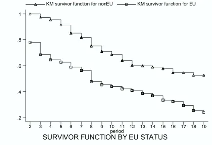
Figure 5.1.1 displays the survivor function conditional on staying for one period (two years) according to EU status.17 _{There is a signiÞcant dierence in the return behavior of EU and}

non-EU migrants. Migrants from wealthier countries (EU countries) are more likely to go back. Conditional on staying for 2 years, 45% of the non-EU migrants return within the next 40 years while around 75% of the EU migrants return.

SURVIVOR FUNCTION BY EU STATUS

period

KM survivor function for nonEU KM survivor function for EU

2 3 4 5 6 7 8 9 10 11 12 13 14 15 16 17 18 19 .2 .4 .6 .8 1 FIGURE 5.1.1

In order to examine the dierences in the timing of return migration according to EU status, we next compare the hazard functions.

17_{We do not show it for the 1st period and after the 19th period because the sample sizes are too small.}

In addition, for non-EU migrants, return at very early years of residence may not be a choice but rather an obligation. (One can apply for permanent residence permits after 5 years.) Among the non-EU migrants, the earliest return we observe is at the 2nd period (2-4 years). Therefore, it is assumed that somebody who survives 2 years in Germany can freely make his return choice. Paine (1974) reports that, in practice, migrants who survived theÞrst couple of years in Germany were able to stay.

HAZARD CONTRIBUTION BY EU STATUS period

Hazard contribution for EU Hazard contribution for nonEU

2 3 4 5 6 7 8 9 10 11 12 13 14 15 16 17 18 19

0 .1 .2

FIGURE 5.1.2

Figure 5.1.2 displays a comparison of the Kaplan-Meier hazard functions according to EU status. We see a dierence in the hazard rates of EU and non-EU migrants up to the 4th period (within theÞrst 8 years) and again after 13th period (after 24 years of residence). Between 8 to 24 years of residence, there is no signiÞcant dierence in the return behavior according to the EU status. Higher return rates in earlier periods for EU migrants suggests that disappointment factor plays a stronger role in the return of EU migrants. Since the opportunity cost of returning, the wage dierential between Germany and the home country, is smaller for EU migrants, there is a smaller dierence between the value of staying and value of leaving. Therefore, a negative shock to either the earnings or the preferences is more likely to push the value of leaving above the value of staying. Another important dierence in the hazard functions is that while the return rates show a downward trend for non-EU migrants after 11th period, they actually increase for EU migrants.

5.2

SAVINGS DECISION

Figures 5.2.1 and 5.2.2 display savings and income proÞles of all immigrants by quartiles18

Savings of immigrants demonstrate a clear downward trend over their duration of residence. Their income levels play no role in this decline as we can see from the income graph that mi-grants’ median income, in fact, rises until the 11th period. The savings proÞle of immigrants

18_{We have no information on savings for less than 5 periods since the survey contains this information}

is relatively constant between the 9th and 16th periods, before decreasing again after 16th period. During this stage, after 10 periods, savings behavior is more parallel with income levels. SAVINGS BY QUARTILES period (p 50) savings (p 75) savings (p 25) savings 5 6 7 8 9 10 11 12 13 14 15 16 17 18 19 20 0 8000 16000 24000 32000 FIGURE 5.2.1

INCOME - ALL MIGRANTS period (p 50) income (p 75) income (p 25) income 5 6 7 8 9 10 11 12 13 14 15 16 17 18 19 20 40000 60000 80000 100000 FIGURE 5.2.2

Selection in return migration could be one reason for the decrease in immigrants’ savings. If the return is in fact part of an optimal life cycle plan of asset accumulation in the host country, we would expect the returners to save more than the stayers. After the 10th period, this trend becomes much weaker as the fraction of people with high propensity to return in

the sample decreases. Now, most migrants’ savings behavior is more like natives’ savings behavior. It more closely follows their income proÞle and there is a downward trend at old age.

One confounding factor may be the time eects on migrants’ income. A higher fraction of the people for whom we utilize the information to draw the above graph on the left-hand side come from later year-of-entry cohorts. Therefore, they potentially have higher lifetime incomes which would allow them to save more. However, the initial downward trend is too precipitous for this to be the case and this would not explain why the proÞle levels o after some time before decreasing at the end again.

5.2.1 Savings By EU Status

A disaggregation of savings and income behavior according to immigrants’ EU status is illustrated below in Figures 5.2.3 and 5.2.4. The most striking fact when we compare the savings behavior of EU and non-EU migrants is the dierence in the proÞles over duration over residence. There is a signiÞcant decrease in the savings of non-EU migrants while the savings of EU migrants seem to be relatively constant over time. Between the 5th and 8th periods, non-EU migrants save on average more than EU migrants even though their income levels are very similar. However, after the 11th period, EU migrants save more than non-EU migrants despite similar levels of income on average.

MEDIAN INCOME BY EU STATUS period EU NON-EU 5-6 7 8 9 10 11 12 13 14 15 16 17+ 60000 70000 80000 FIGURE 5.2.3

MEDIAN SAVINGS BY EU STATUS period EU NON-EU 5-6 7 8 9 10 11 12 13 14 15 16 17+ 0 4000 8000 12000 FIGURE 5.2.4

This savings behavior seems to be consistent with the hazard rates shown above in a model where the motivation to return comes from accumulated assets. The hazard function for the non-EU migrants reaches the peak of its hump at the 8th period. What we see in the above savings proÞle is that their savings are the highest before 8th period. After the 8th period, as the savings proÞle moves downward, the return rate also goes down for non-EU migrants. After the 12th period, both the return rates and savings of non-EU migrants are much lower than those of EU migrants. This suggests that a much smaller fraction of people with high propensity to return is left in the sample for non-EU migrants during this time. On the other hand, the hazard function for EU migrants displays an increase after the 12th period. When we look at their savings behavior, we see that EU migrants maintain their previous level of savings in this interval. This suggests that unlike the non-EU migrants, there still exists a sizeable proportion of returners in the pool of EU migrants even after the 12th period.

6

ESTIMATION METHOD

• the return migration choice made by the migrant. (mt)

• the savings choice made by the migrant. (At+1At)

• the earnings of the migrant. (yt)

• the labor market status of the migrant. (lt)

Let {Oi} = {Di, Xi} denote observed outcomes for individual i, where Di = {dit} =

{{mit},{AitAit31}}is the history of observed choices and Xi = {xit} = {{lit},{yit}} is

the history of observed exogenous covariates. The data are:

W hen mTi = 1 O obs i ={{mit}Tt=1i ,{AitAit31}Tt=i3ti,11991,{lit} Ti31 t=1 ,{yit}Tt=i3ti,11983} W hen mTi = 0 O obs i ={{mit}Tt=1i ,{AitAit31}Tt=iti,1991,{lit} Ti t=1,{yit}Tt=iti,1983}

whereti,19xxis the period number for individual i in 19xx andTiis the last period in the

sample for individual i. If the return choice is to leave, for that period we do not observe the other outcomes.

One of the endogenous state variables, assets, is not observed. Therefore, we use the method introduced by Keane and Wolpin (2001) for estimating dynamic panel data models with unobserved endogenous state variables. Typically, calculation of the probabilities that form the likelihood function requires conditioning on past state variables. The novel feature of this method is that it obviates the need to calculate these conditional probabilities. The underlying idea of this estimation method is to minimize the distance between the simulated and reported outcomes. A measure of the distance between the simulated and reported outcomes is constructed by assuming that the observed outcomes are measured with error. In a recent paper, Keane and Sauer (2003) show that this estimator has good small sample properties in a more extended setting.

The key assumption, therefore, is that the observed outcomes are measured with error. By acknowledging the existence of measurement errors (classiÞcation errors in the case of discrete outcomes), we are incorporating into our likelihood calculation, for instance, the

fact that when a migrant is observed as employed, there is a positive probability that he was in fact unemployed, but his employment status was classiÞed incorrectly in the data. In the case of observed earnings and savings, we take a similar approach; however, in this case the measurement errors have continuous distributions.

6.1

Generation of Simulated Outcomes

• For each individual and period, draw N shocks. n©{0t}Tt=1i

ªN n=1

oI i=1

• Using the initial state variables and sequence of shocks drawn, simulate N choice histories,©{mt,(At+1At)}Tt=1i

ªN

n=1 = D

sim_{, and histories for exogenous covariates,}

©

{et, yt}Tt=1t

ªN

n=1= X

sim _{for each individual i.}

• Using the simulated values19_{, construct the unbiased classiÞcation error rates for the}

discrete outcomes. (See Appendix B for the speciÞcations of these classiÞcation errors.)

6.2

Likelihood Function

The contribution to the likelihood of individual i is calculated by the below simulator, which is the probability of observing the reported outcomes conditional on the simulated outcomes averaged over the N simulated choice histories.

19_{We do not have information on assets at the time of entry to Germany. The very fact that these}

people chose to immigrate to Germany suggests that they did not hold signiÞcant assets when they entered Germany. However, in order to capture the dierences in this that may arise due to dierences at age of entry or country of origin, we write it as a deterministic function in these two variables.

A0=0+1I(z3) +2age0+3age0I(z3)

b P(Oobs_i ) = N P n=1 P((Dobs

i , Xiobs)|(Dsimin , Xinsim)) N

P

n=1

I({mit}tt1983=1 = 0)

Note that P((Dobs

i , Xiobs)|(Dsimin , Xinsim) is not conditional on any of the state variables.

Therefore, we can calculate this probability even if we do not observe some of the state variables.

Unobserved heterogeneity enters the estimation in the following way: We assume that there is a Þnite number (K) of type groups. Each individual i may belong to any of these type groups, 1 to K. It is the probability of being a certain type that diers across individu-als. Therefore, when we generate the simulated outcomes for individual i and calculate the above simulator, we do it for all types. Then, the likelihood contribution for this individual is calculated as the weighted average of the above simulator over the probabilities of his belonging to each type.

b P(Oobs i ) = K X k=1 Vi,k 3 E E E C N/K_P n=1 P(Oobs i )|(Osimikn)) N/K_P n=1 I({mit}tt1983=1 = 0) 4 F F F D

whereVi,k, the probability of individual i being of type k, is speciÞed as a logit with age

at entry and country of origin as arguments.

Vk =V(age0, z, t1983)

The probability of observing the reported spells conditional on the simulated spells can be written as follows.

P((D_iobs, X_iobs)|(D_insim, X_insim)) =

P(M_iobs|M_insim)

Ti

Y

t=1

Pr(AitAit31)obs|(AintAint31)sim] Pr(yitobs|yintsim) Pr(lobsit |lsimint )

We use the measurement error distributions and classiÞcation error rates to calculate these probabilities. See appendix B for these calculations. For the optimization method, we use the Downhill Simplex Algorithm.

7

RESULTS

In this section, we present our maximum likelihood estimation results based on the full solution of the dynamic model.

7.1

Model Fit

We Þrst illustrate and discuss how our model’s predictions as to the return migration and savings behavior of immigrants Þt the observed features of the data.

7.1.1 Return Migration

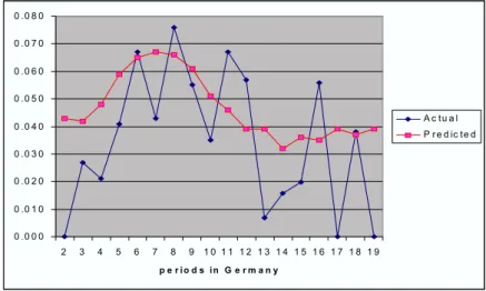
Hazard Contribution By EU Status Figure 7.1.1 compares the actual and predicted hazard contribution for non-EU immigrants Both the level and the shape of the predicted hazard function match the data reasonably well. Our model certainly captures the hump shape of the hazard function. The only signiÞcant dierence between the actual and predicted hazard rates exist within the Þrst 5 periods. The sample size is rather small in this range since most of the immigrants in our sample entered Germany before 1973. The low hazard rates in the sample is probably due to the size of the sample.20

FIGURE 7.1.1: HAZARD CONTRIBUTION FOR NON-EU IMMIGRANTS

0 .0 0 0 0 .0 1 0 0 .0 2 0 0 .0 3 0 0 .0 4 0 0 .0 5 0 0 .0 6 0 0 .0 7 0 0 .0 8 0 2 3 4 5 6 7 8 9 1 0 1 1 1 2 1 3 1 4 1 5 1 6 1 7 1 8 1 9 p e r i o d s i n G e r m a n y A c t u a l P r e d ic t e d

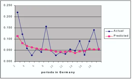
The model matches the hazard function of EU migrants well as shown below in Figure 7.1.2. It captures the decreasing proÞle in the early part of the graph. The predicted levels in

the 2nd and 3rd periods are somewhat lower, though.21 _{The model also matches the steady}

hazard rates around 5% in the middle part of the graph. Even though the predicted hazard rates exhibit an increase after the 15th period, it is weaker compared to what we observe in the data. The spike in the data after the 15th period could also be due to the smaller sample size in this range.

FIGURE 7.1.2: HAZARD CONTRIBUTION FOR EU IMMIGRANTS

0 . 0 0 0 0 . 0 5 0 0 . 1 0 0 0 . 1 5 0 0 . 2 0 0 0 . 2 5 0 2 4 6 8 _{10 12 14 16 18} p e r i o d s i n G e r m a n y A c t u a l P re d ic t e d

Survival Rates By Nationality In Table 7.1.1, the model’s predictions on survivor rates after 20 periods are compared to the actual values by nationality. 22 _{As can be seen from}

the table, the predictions match the actual values very well for all nationalities.

TABLE 7.1.1: SURVIVOR RATES AFTER 40 YEARS

Turkish Yugoslavian Greek Italian Spanish

Actual* 30.4% 58.7% 22.6% 30.7% 21.5%

Predicted 30.0% 57.7% 22.4% 30.5% 22.0%

* Actual values are parametric (log-logistic).

7.1.2 Savings

Figures 7.1.3 and 7.1.4 display how the predicted savings from our model compare to the actual savings according to immigrants’ EU status.

21_{The sample size is small for these periods.}

22_{The actual survivor rates are parametric as the sample size by nationality is too small to calculate}

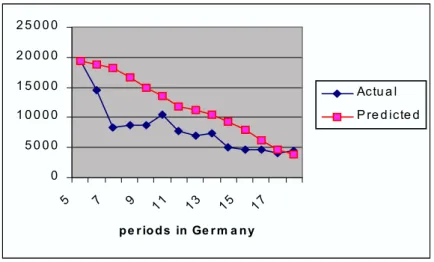
FIGURE 7.1.3:MEAN SAVINGS FOR NON-EU IMMIGRANTS 0 5 0 0 0 1 0 0 0 0 1 5 0 0 0 2 0 0 0 0 2 5 0 0 0 5 7 9 ₁1 ₁3 ₁5 ₁7 p e r io d s in Ge r m a n y Ac tu a l P re d ic te d

Our model captures the downward sloping proÞle of the mean savings of non-EU migrants. However, the level of savings is signiÞcantly overpredicted between the 7th and 10th periods and somewhat overpredicted between the 11th and 17th periods. In terms ofÞtting the level of savings, we do much better with the EU migrants. Except for the 8th and 9th periods, our predictions are close the values in the data. In addition, our model also captures the ßatness of the savings of the EU migrants until the 16th period -there is a somewhat of a slope at the beginning in our predictions, though-.as well as the downward slope after that.

FIGURE 7.1.4:MEAN SAVINGS FOR EU IMMIGRANTS

0 2 0 0 0 4 0 0 0 6 0 0 0 8 0 0 0 1 0 0 0 0 1 2 0 0 0 1 4 0 0 0 1 6 0 0 0 6 8 ₁0 ₁2 ₁4 ₁6 ₁8 p e r i o d s i n G e r m a n y A c t u a l P re d ic t e d

7.2

Interpretation of Types

There are two types of immigrants, distinguished with respect to their permanent character-istics as to their psychic cost of living in Germany, their risk aversion and bequest motive. The estimated parameters indicate that type 1’s have a higher psychic cost at time zero that decreases at a faster rate by duration of residence in Germany. Their psychic cost at all periods of residence is higher despite the faster decline. Type 1’s are also more risk averse; but have a weaker bequest motive.

In order to better understand the dynamics underlying the return migration and savings behavior of immigrants illustrated above and to interpret the results of the policy experiments of next section, we should understand the dierences in the behavior of the two types. We should also keep in mind that dierences in the out-migration rates change the percentage of each type in the population over time.

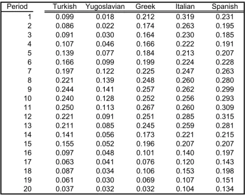
Table 7.2.1 reports the hazard contribution for type 1 immigrants. Examining the hazard rates of type 1 immigrants reveals a hump-shaped proÞle. The peak of the hump varies by nationality. For non-EU migrants who face lower prices after return, the peak takes place earlier (9th to10th periods) compared to that for EU migrants(11th to 12th periods). The level of the hazard rates and the peak is higher for EU migrants. We also observe that the hazard rates for EU migrants in the earlier periods are very high. The biggest dierence between the hazard rates of EU and non-EU migrants is in these earlier periods. This dierence dies down as the number of periods increases. Another interesting fact is that even though the survivor rate of type 1 Spanish immigrants after 20 periods (0.6%) is lower than that for type 1 Italian immigrants (0.7%), the hazard rate in the initial periods for Italian migrants is much higher. This is mostly due to higher expected earnings in Italy. In the initial periods -when most of the immigrants are young-, the expected earnings back at home has a stronger bite.

TABLE 7.2.1: HAZARD CONTRIBUTION OF TYPE 1 IMMIGRANTS Period Turkish Yugoslavian Greek Italian Spanish

1 0.099 0.018 0.212 0.319 0.231 2 0.086 0.022 0.174 0.263 0.195 3 0.091 0.030 0.164 0.230 0.185 4 0.107 0.046 0.166 0.222 0.191 5 0.139 0.077 0.184 0.213 0.207 6 0.166 0.099 0.199 0.224 0.228 7 0.197 0.122 0.225 0.247 0.263 8 0.221 0.139 0.248 0.260 0.280 9 0.244 0.141 0.257 0.262 0.299 10 0.240 0.128 0.252 0.256 0.293 11 0.250 0.113 0.267 0.260 0.309 12 0.221 0.091 0.251 0.285 0.315 13 0.211 0.085 0.245 0.259 0.281 14 0.141 0.056 0.173 0.221 0.215 15 0.155 0.052 0.196 0.207 0.207 16 0.097 0.048 0.101 0.140 0.197 17 0.063 0.041 0.076 0.120 0.143 18 0.087 0.034 0.106 0.153 0.198 19 0.061 0.030 0.069 0.107 0.151 20 0.037 0.032 0.032 0.104 0.134

On the other hand, the hazard rates of type 2 immigrants are much lower. As can be seen from Table 7.2.2, even after 40 years of residence, more than half of the type 2 immigrants remain in Germany for all nationalities. This implies that as the number periods increase, the fraction of type 2 immigrants will increase as well. As a result, the behavioral features of type 2 immigrants will start to dominate. Since the hazard rates for type 1 EU immigrants are higher, this eect will be stronger for EU immigrants.

TABLE 7.2.2: SURVIVOR RATES AFTER 40 YEARS BY TYPE Turkish Yugoslavian Greek Italian Spanish

Type 1 0.040 0.229 0.018 0.007 0.006

Type 2 0.631 0.864 0.544 0.531 0.530

When we examined the hazard functions according to migrants’ EU status, we observed that non-EU migrants of all types had a hump-shaped hazard proÞle whereas EU migrants of all types had a downward sloping proÞle that got leveled o after some time. The reason to this is the change in the type composition as explained in the above paragraph. As can be seen from Table 7.2.3, the out-selection of type 1 immigrants is stronger among EU immigrants; therefore, the hazard rates of type 2 immigrants start to dominate much earlier, pulling the hump-shaped proÞle of type 1 immigrants to much lower levels. In addition to

that, the hump of the type 1 EU immigrants take place at a later period compared to the hump of type 1 non-EU immigrants; therefore, there has been stronger out-selection of type 1 EU immigrants during the hump range.

TABLE 7.2.3: PROPORTION OF TYPE 1 IMMIGRANTS BY PERIOD period Turkish Yugoslavian Greek Italian Spanish

0 0.768 0.537 0.868 0.530 0.834 4 0.690 0.509 0.753 0.266 0.680 8 0.506 0.396 0.550 0.118 0.423 12 0.271 0.285 0.294 0.042 0.160 16 0.182 0.244 0.184 0.020 0.074 20 0.175 0.235 0.176 0.015 0.051

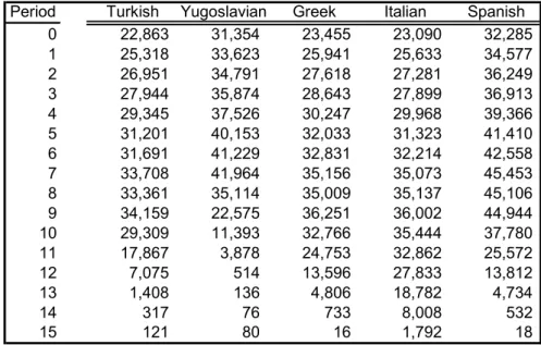
Table 7.2.4 reports the mean savings of type 1 immigrants. Given their income and minimum consumption level determined by their family size, these immigrants basically save whatever they can. On average, their savings rate is almost around 40% till the 10th period.

23 _{Spanish and Yugoslavian immigrants can save more each period mainly due to their}

higher earnings and smaller family size. Another important thing to notice in this table is the timing of the fast decline. The decline takes place earlier for Turkish and Yugoslavian immigrants who face lower prices after they return to their home country.

TABLE 7.2.4: MEAN SAVINGS OF TYPE 1 IMMIGRANTS Period Turkish Yugoslavian Greek Italian Spanish

0 22,863 31,354 23,455 23,090 32,285 1 25,318 33,623 25,941 25,633 34,577 2 26,951 34,791 27,618 27,281 36,249 3 27,944 35,874 28,643 27,899 36,913 4 29,345 37,526 30,247 29,968 39,366 5 31,201 40,153 32,033 31,323 41,410 6 31,691 41,229 32,831 32,214 42,558 7 33,708 41,964 35,156 35,073 45,453 8 33,361 35,114 35,009 35,137 45,106 9 34,159 22,575 36,251 36,002 44,944 10 29,309 11,393 32,766 35,444 37,780 11 17,867 3,878 24,753 32,862 25,572 12 7,075 514 13,596 27,833 13,812 13 1,408 136 4,806 18,782 4,734 14 317 76 733 8,008 532 15 121 80 16 1,792 18

23_{In fact, such high savings rates have been reported in the literature of guest-workers. (Kumcu,}

On the other hand, the savings proÞle of type 2’s is ratherßat and the levels are much lower. Per period savings of type 2 immigrants of all nationalities never exceed 15,000DM and are lower than 10,000DM for most of the range. The reason that we observe a stronger downward slope in the savings proÞle of non-EU immigrants is the same reason as above. Since type1 EU immigrants have higher hazard rates compared to type 1 non-EU immigrants, non-EU migrants have a higher fraction of type 1’s left after the 5th period . As a result, the savings behavior of type 1 immigrants, a downward sloping proÞle, is more prominent among the non-EU migrants.

7.3

Implications of the Results

Here, we discuss two important implications of immigrants’ return and savings behavior. One is important from the host country’s perpective, the timing of immigrants’ return pertaining to the social security system in the host country, and the other is important from the source countries’ perpective, how much assets immigrants bring with them when they return.

7.3.1 Social Security Contributions and BeneÞts

An important policy question from the host country’s perpective is what fraction of these immigrants leave before they qualify for pension beneÞts. Table 7.3.1 presents the cumulative hazard rates -one minus the survival rates- by the end of second and third periods. The reason we choose the second and third periods is that, in Germany, the minimum number of years of labor market experience to qualify for pension beneÞts is 5 years. All immigrants who left by the end of the second period (within the Þrst 4 years) did not qualify before they left. Some of the immigrants who left in the third period (Þfth or sixth year of residence in Germany) did not qualify as well.

TABLE 7.3.1: CUMULATIVE HAZARD RATES

EU Non-EU

2nd period 27.7% 9.3% 3rd period 33.7% 13.1%

As we see from the above table, almost a third of EU immigrants leave before they qualify; whereas, the fraction is around one tenth for non-EU immigrants. Of course, in terms of immigrants contributions and withdrawals from the social security contribution, the timing of return of immigrants is important even after they qualfy for beneÞts because although an

immigrant who returns after 6 years of residence24 _{will receive beneÞts, these beneÞts will}

be very small.

7.3.2 Asset Accumulation

Figure 7.3.1 compares the asset levels of stayers and returners for Turkish immigrants. We see that immigrants who choose to return hold signiÞcantly higher assets. Although it is shown here only for Turkish immigrants, it holds for all other nationalities as well.

We observe a peak because in that range most of the leavers are type 1 immigrants, who have high propensity to save and those who leave at later periods have higher assets simply because they took a longer time to do so. However, as type 1 immigrants get older and there remains a shorter lifetime horizon, their savings rate goes down. In addition, among the type 1’s, the ones with higher assets are selected (already returned). Therefore, their asset proÞle becomesßatter and eventually goes down. Moreover, at later periods there is a higher proportion of type 2 immigrants among the returners. Because of these three factors, the assets proÞles of returners take a sharp downturn.

FIGURE 7.3.1: ASSET LEVELS OF STAYERS AND RETURNERS: TURK-ISH IMMIGRANTS 0 5 0 0 0 0 1 0 0 0 0 0 1 5 0 0 0 0 2 0 0 0 0 0 2 5 0 0 0 0 3 0 0 0 0 0 1 4 7 ₁0 ₁3 ₁6 ₁9 p e r io d s in Ge r m a n y S ta ye rs R e tu rn e rs

Table 7.3.2 reports the average asset level of a returner (which is calculated by weighting the values in the above graph by the hazard rates). Even though the average level of assets

24_{Since everybody is willing to be employed in our model, duration of residence is equal to the duration}

in the labor market. In Germany, periods of unemployment are included in the social security contribution period.

of a Spanish return migrant is lower than that of non-EU returners, when we look at the assets proÞle of the returners over duration of residence, we see that at each period Spanish return migrants take home more assets. However, the average over the all periods is lower because a much higher fraction of Spanish immigrants return home at the early periods.

TABLE 7.3.2: AVERAGE ASSET LEVEL OF A RETURNER Turkish Yugoslavian Greek Italian Spanish

156,085

193,955 130,363 115,548 153,922

Table 7.3.3 reports the average assets that return to the host country from all immigrants that leave for the host country. Spanish workers who leave their country to work in the host country bring back the highest amount of assets because they are more likely to return and their returners accumulate more assets in the host country. Despite the fact that Greek immigrants are more likely to return compared to Turkish immigrants, Turkish immigrants bring back more due to higher assets of their returners.

TABLE 7.3.3: AVERAGE RETURN ASSET LEVEL FROM ALL IMMI-GRANTS

Turkish Yugoslavian Greek Italian Spanish 109,260

82,043 101,162 80,306 120,059

8

POLICY EXPERIMENTS

8.1

Changes in the Replacement Rate of Unemployment Bene

Þ

ts

Table 8.1.1 reports how the return behavior of immigrants respond to the changes in the replacement rate of the unemployment compensation system. The experiments indicate that migrants’ return decision is relatively sensitive to the replacement rate. A drop in the replacement rate from 0.6 to 0.5 decreases the survivor rate after 40 years among Turkish migrants from 30.0% to 28.6%. Although the unemployment rate among the Italian and Spanish immigrants is much lower, this policy is almost as eective in decreasing their survivor rate. It goes down from 30.5% to 29.3% for Italian immigrants and from 22.0% to 21.4% for Spanish immigrants. On the other hand, the policy is much less eective with the Yugoslavian workers despite their higher unemployment rates compared to the Italian and Spanish immigrants.

Decreasing the replacement rate further below 0.5 to 0.4 has no eect on the survivor rate of Turkish immigrants whereas it is still eective on the Italian and Spanish immigrants. This result is due to the social assistance that the German government provides which makes sure that immigrants’ income do not fall below the subsistence level. As shown in the model section, this assistance depends on migrants’ family size. Since Turkish migrants have on average larger families, their subsistence income is higher. Consequently, as we decrease the unemployment replacement rate, this subsistence income becomes binding at a higher replacement rate for Turkish immigrants. For instance, decreasing the replacement rate even more to 0.3 has little eect on the survivor rate of any immigrant group. Once we lower it to 0.2, there is no eect at all.

TABLE 8.1.1: EFFECT OF REPLACEMENT RATE ON THE SURVIVOR RATE AFTER 40 YEARS

Turkish Yugoslavian Greek Italian Spanish 0.6(Baseline) 30.0% 57.7% 22.4% 30.5% 22.0% 0.55 29.3% 57.5% 22.2% 29.9% 21.7% 0.5 28.6% 57.2% 22.1% 29.3% 21.4% 0.4 28.6% 56.7% 22.0% 28.6% 20.7% 0.3 28.6% 56.5% 22.0% 28.6% 20.6% 0.2 28.6% 56.5% 22.0% 28.6% 20.6%

The interesting result from this policy experiment is that it has a stronger impact on immigrants from EU countries despite their lower unemployment rates. One reason to this, as explained above, is the fact that the subsistence beneÞts EU migrants receive is lower due to their smaller family size. As a result, the policy changes the income levels of a larger fraction of EU migrants. However, even before the subsistence income becomes binding, when we decrease the replacement rate to 0.5, for Italian and Spanish immigrants the program is more eective compared to Yugoslavian immigrants, who have higher unemployment rates, and as much eective as it is for Turkish immigrants, who have much higher unemployment rates. Understanding this result requires further investigation of the eect of the policy experiment by type.

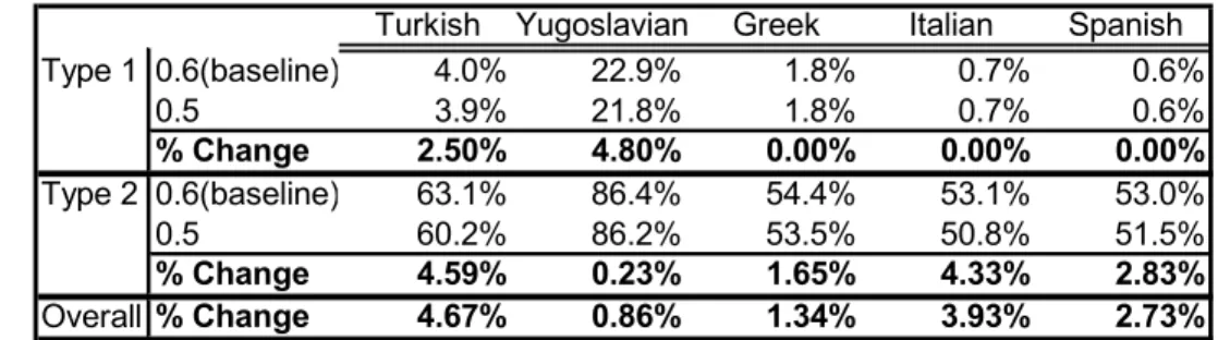
TABLE 8.1.2: EFFECT OF REPLACEMENT RATE ON THE SURVIVOR RATE AFTER 40 YEARS BY TYPE

Turkish Yugoslavian Greek Italian Spanish

Type 1 0.6(baseline) 4.0% 22.9% 1.8% 0.7% 0.6% 0.5 3.9% 21.8% 1.8% 0.7% 0.6% % Change 2.50% 4.80% 0.00% 0.00% 0.00% Type 2 0.6(baseline) 63.1% 86.4% 54.4% 53.1% 53.0% 0.5 60.2% 86.2% 53.5% 50.8% 51.5% % Change 4.59% 0.23% 1.65% 4.33% 2.83% Overall % Change 4.67% 0.86% 1.34% 3.93% 2.73%

As can be seen in Table 8.1.2, a decrease in the replacement rate from 0.6 to 0.5 has a stronger eect on type 2 immigrants of all nationalities except for Yugoslavian immigrants. Since most of the type 1 immigrants choose to return within the 40 year period anyway, the policy has a lesser eect on them.

At Þrst, one might think that the stronger impact of the policy on Italian and Spanish immigrants compared to Yugoslavian immigrants -despite the higher unemployment rates among the latter group- would be due to the dierences in the type proportions. In the above table, we see that type 2 immigrants are more responsive to the policy and there is a larger fraction of type 2 Italian immigrants at any period and a larger fraction type 2 Spanish immigrants after the 9th period when the unemployment rates start to peak. This fact is true; however, there is a secondary eect as well.

Even when we condition on type 2 immigrants, we see that the impact of the policy is much stronger for Italian and Spanish immigrants compared to Yugoslavian immigrants. The reason to this is the dierence between the value of spending the rest of one’s life in his home country and the value of staying in Germany. This dierence is much smaller for type 2 Italian and Spanish immigrants. Therefore, a decrease in the value of staying in Germany due to smaller unemployment beneÞts has a stronger bite in the return decisions of these migrants. It is the same reason why the policy is not so much more eective for Turks. However, compared to Yugoslavian immigrants, Turks response is stronger because the unemployment rate among them is higher and the dierence between the value functions is not as acute as that for the Yugoslavian immigrants.

We would expect the additional returners -people who are induced to return as a result of the change in the compensation system- to be selected from immigrants that are more likely to be unemployed; thereby, decreasing the unemployment rates of immigrants that stay. The below table compares the unemployment rates of Italian immigrants under dierent

replacement rates. What weÞnd is that the impact of a decrease in the replacement rate on the unemployment rates of immigrants is negligible.

8.2

Financial Bonuses to Encourage Return

8.2.1 Bonuses Given Before Migrants Qualify for Pension BeneÞts

Financial bonuses given to immigrants conditional on return to their home country at the end of second period (4 years of residence) would relieve the host country from paying pension beneÞts to these immigrants. Table 8.2.1 presents the eect of such bonuses on the hazard rates at the second period. As can be seen from the table, the policy makes a strong impact on the second period hazard rates. The impact of the bonus depends on the purchasing power parity of the source countries with Germany. While a bonus of 10,000DM increases the hazard rate of Turkish immigrants by 35%, it does so only by 17% for Italian immigrants. We also Þnd diminishing returns to the amount of bonuses given. The second and third 10,000DM increment of bonus increase the hazard rate of Italian immigrants by 15% and 13%, respectively.

TABLE 8.2.1: HAZARD RATES AT THE SECOND PERIOD WITH DIF-FERENT BONUSES

Turkish Yugoslavian Greek Italian Spanish

Baseline 6.0% 1.2% 12.0% 10.6% 12.9% 10,000 8.1%(35%) 1.8%(50%) 14.7%(23%) 12.4%(17%) 15.4%(19%) 20,000 10.8%(33%) 2.5%(39%) 17.8%(21%) 14.2%(15%) 18.0%(17%) 30,000 13.9%(29%) 3.5%(40%) 21.0%(18%) 16.0%(13%) 20.7%(15%)

Numbers in paranthesis are percentage changes from previous line.

The impact of thisÞnancial bonus would not be limited to the period it is given, though. Many of the immigrants who choose to accept the Þnancial oer and return to their home country would have done so anyway, albeit later. Figure 8.2.1 shows the impact of a 20,000DM bonus on the hazard function of Turkish immigrants. What we see is that after the spike in the second period as a result of the bonus, the hazard rates are lower compared to the baseline values.

FIGURE 8.2.1: EFFECT OF A BONUS ON THE HAZARD FUNCTION OF TURKISH IMMIGRANTS 0 0.02 0.04 0.06 0.08 0.1 0.12 1 3 5 7 9 1 1 1 3 1 5 1 7 1 9

periods in G erm any

B as eline B onus = 20,000DM

Only some of the immigrants who accept the oer are those who would stay in Germany throughout their lives. In order to see this longer term eect ofÞnancial bonuses, we compare the cumulative hazard rates from the 2nd period, when the Þnancial bonus is given, to the end of the 20th period. Table 8.2.2 reports these cumulative values for the baseline case and for the case with a 30,000DM bonus. When we compare the changes in the cumulative hazard rates with the Þnancial bonus according to nationality groups, we realize that the ordering that we saw in the previous table according to purchasing power parities is lost. In fact, the percentage change is lower for Turkish immigrants compared to all EU nationalities and it is higher for Italian compared to Yugoslavian immigrants.

TABLE 8.2.2: CUMULATIVE HAZARD RATES FROM THE 2ND TO THE 20TH PERIODS

Turkish Yugoslavian Greek Italian Spanish

ALL Baseline 67.5% 41.7% 72.5% 62.8% 72.6% 30,000 68.0% 42.0% 73.0% 63.3% 73.1% Change 0.65% 0.72% 0.68% 0.83% 0.69% Type 1 Baseline 95.6% 76.7% 97.7% 99.0% 99.2% 30,000 96.0% 77.6% 98.1% 99.3% 99.5% Change 0.46% 1.20% 0.39% 0.30% 0.26% Type 2 Baseline 36.8% 13.5% 45.3% 45.7% 46.5% 30,000 37.0% 13.5% 45.5% 46.4% 46.8% Change 0.54% 0.00% 0.44% 1.58% 0.67%

The reason to this becomes clear when we examine the cumulative hazard rates according to the types. Among those who return to their home country, type 2 immigrants contain a