Boltzmann Methods and its Application to
Complex Flows
Vom Fachbereich Maschinenbau und Verfahrenstechnik der Technischen Universität Kaiserslautern
zur Verleihung des akademischen Grades
Doktor-Ingenieur (Dr.-Ing.)
genehmigteDissertation
von
Herrn
Dipl.-Ing. Andreas Schneider
aus Landstuhl
Tag der mündlichen Prüfung: 23. März 2015
Dekan: Prof. Dr.-Ing. Christian Schindler Vorsitzender: Prof. Dr.-Ing. Sergiy Antonyuk Berichterstatter: Prof. Dr.-Ing. Martin Böhle
Prof. Dr.-Ing. habil. Uwe Janoske
Die vorliegende Arbeit entstand während meiner Tätigkeit als wissenschaftlicher Mitarbeiter am Lehrstuhl für Strömungsmechanik und Strömungsmaschinen der Technischen Universität Kaiserslautern.
Mein besonderer Dank gilt Herrn Prof. Dr.-Ing. Martin Böhle für die steten Anregungen, Dis-kussionen und Ratschläge, die wesentlich zum Gelingen dieser Arbeit beigetragen haben.
Ebenfalls bedanke ich mich bei Herrn Prof. Dr.-Ing. habil. Uwe Janoske für die Übernahme des Koreferats und bei Herrn Prof. Dr.-Ing. Sergiy Antonyuk für die Übernahme des Vorsitzes der Prüfungskommision.
Den Kolleginnen und Kollegen am Lehrstuhl für Strömungsmechanik und Strömungsmaschi-nen danke ich für das angenehme, sehr kollegiale Arbeitsklima und für viele freundschaftliche Gespräche. Meinen studentischen Hilfskräften und Studien- und Diplomarbeitern danke ich für ihre tatkräftige Mithilfe.
Größten Dank spreche ich meinem Kollegen und Freund Daniel Conrad für die tolle Zusam-menarbeit und die Unterstützung in allen Lebenslagen aus.
Ein großer Dank gilt auch meiner Familie und meinen Freunden. Meinen Eltern Werner und Sonja dafür, dass sie mir eine hervorragende Ausbildung ermöglicht haben und mich bei mei-nen Entscheidungen und meinem Handeln immer unterstützt haben. Meimei-nen Brüdern Mathias und Marcel für ihr Vertrauen in mich und für viele Ratschläge. Allen meinen Freunden danke ich für ihren Beistand und ihre Unterstützung auch in schwierigen Zeiten.
Kaiserslautern, im April 2015 Andreas Schneider
Vorwort iii
Abstract ix
Kurzfassung auf Deutsch xi
1 Introduction 1
1.1 Motivation . . . 1
1.2 Scope of this Thesis . . . 2
1.3 Physical Description of Fluid Flows . . . 3
1.4 Mathematical Notation . . . 4
2 Kinetic Theory 7 2.1 The Distribution Function . . . 7
2.2 The Boltzmann Equation . . . 9
2.3 The Equilibrium Distribution Function . . . 10
2.4 BGK Approximation . . . 11
2.5 The Chapman-Enskog Expansion . . . 12
3 The Lattice Boltzmann Method 15 3.1 The Lattice Boltzmann Equation . . . 15
3.1.1 Discretization of Velocity Space . . . 16
3.1.2 Discretization in Space and Time . . . 18
3.2 Discrete Phase Space Model . . . 21
3.3 Collision Operators . . . 24
3.3.1 Single Relaxation Time Model . . . 24
3.3.2 Multiple Relaxation Time Model . . . 25
3.4 Treatment of External Forces . . . 27
3.4.1 Single Relaxation Time Model . . . 27
3.4.2 Multiple Relaxation Time Model . . . 28
3.5 Boundary Conditions . . . 29
3.5.1 Equilibrium Schemes . . . 29
3.5.2 Periodic Boundary Conditions . . . 29
3.5.3 Bounce Back Schemes . . . 30
3.5.4 Bouzidi Scheme . . . 32 3.5.5 Yu Scheme . . . 33 3.5.6 Mei Scheme . . . 35 3.5.7 Shear Boundaries . . . 35 3.6 Initial Conditions . . . 41 3.6.1 Analytical Schemes . . . 41 3.6.2 Iterative Schemes . . . 41
3.7 Local Grid Refinement . . . 41
3.7.1 General Concept . . . 42
3.7.2 SRT Scaling . . . 46
3.7.3 MRT Scaling . . . 47
3.7.4 Nested Time Stepping . . . 48
3.8 Accuracy and Stability . . . 48
3.8.1 Accuracy Issues . . . 48
3.8.2 Stability Issues . . . 50
4 Large Eddy Simulation for Lattice Boltzmann Methods 53 4.1 Principles of Large Eddy Simulation . . . 53
4.2 Application to the Lattice Boltzmann Method . . . 56
4.2.1 Filtered Lattice Boltzmann Equation . . . 57
4.2.2 Subgrid Scale Models . . . 59
4.3 Boundary Conditions for Large Eddy Simulation . . . 61
4.3.1 Wall Boundary Conditions . . . 61
4.3.2 Inlet Boundary Conditions . . . 69
4.4 Grid Refinement for Large Eddy Simulation . . . 74
4.5 Practical Aspects for Large Eddy Simulation . . . 75
5 Implementation Aspects of the CFD Package SAM-Lattice 77 5.1 Conceptual Aspects . . . 77
5.2 Preprocessor - SamGenerator . . . 78
5.2.1 Input Data . . . 80
5.2.2 Discretization of Grid Level 0 . . . 80
5.2.4 Lattice Definition . . . 82 5.2.5 Output Data . . . 83 5.3 Solver - SamSolver . . . 83 5.3.1 Input Data . . . 84 5.3.2 Preprocessing . . . 86 5.3.3 Solving . . . 86 5.3.4 Output Data . . . 87 6 Verification Cases 89 6.1 Core Components . . . 90 6.1.1 Beltrami Flow . . . 90 6.1.2 Taylor-Couette Flow . . . 95 6.1.3 Couette Flow . . . 99 6.1.4 Jeffery-Hamel Flow . . . 104 6.2 LES Components . . . 108
6.2.1 Wall Resolved Approach . . . 108
6.2.2 Wall Modeled Approach . . . 113
6.2.3 Synthetic Eddy Method . . . 119
7 Pump Intake Flows - Complex Validation Cases 123 7.1 Pump Intakes . . . 123
7.2 Free Surface Intake . . . 128
7.3 Pressurized Intake . . . 137
8 Conclusions and Future Work 153
A D3Q19 MRT Model 155 Nomenclature 159 List of Figures 163 List of Tables 167 Bibliography 169 Curriculum Vitae 179
Lattice Boltzmann Methods have shown to be promising tools for solving fluid flow problems. This is related to the advantages of these methods, which are among others, the simplicity in handling complex geometries and the high efficiency in calculating transient flows. Lattice Boltzmann Methods are mesoscopic methods, based on discrete particle dynamics. This is in contrast to conventional Computational Fluid Dynamics methods, which are based on the so-lution of the continuum equations. Calculations of turbulent flows in engineering depend in general on modeling, since resolving of all turbulent scales is and will be in near future far beyond the computational possibilities. One of the most auspicious modeling approaches is the large eddy simulation, in which the large, inhomogeneous turbulence structures are directly computed and the smaller, more homogeneous structures are modeled.
In this thesis, a consistent large eddy approach for the Lattice Boltzmann Method is intro-duced. This large eddy model includes, besides a subgrid scale model, appropriate boundary conditions for wall resolved and wall modeled calculations. It also provides conditions for turbulent domain inlets. For the case of wall modeled simulations, a two layer wall model is derived in the Lattice Boltzmann context. Turbulent inlet conditions are achieved by means of a synthetic turbulence technique within the Lattice Boltzmann Method.
The proposed approach is implemented in the Lattice Boltzmann based CFD package SAM-Lattice, which has been created in the course of this work. SAM-Lattice is feasible of the calculation of incompressible or weakly compressible, isothermal flows of engineering interest in complex three dimensional domains. Special design targets of SAM-Lattice are high autom-atization and high performance.
Validation of the suggested large eddy Lattice Boltzmann scheme is performed for pump intake flows, which have not yet been treated by LBM. Even though, this numerical method is very suitable for this kind of vortical flows in complicated domains. In general, applications of LBM to hydrodynamic engineering problems are rare. The results of the pump intake vali-dation cases reveal that the proposed numerical approach is able to represent qualitatively and quantitatively the very complex flows in the intakes. The findings provided in this thesis can serve as the basis for a broader application of LBM in hydrodynamic engineering problems.
Seit einiger Zeit zeigen die Tendenzen im Ingenieurwesen, dass die Produktentwicklung und Herstellung zunehmend von rechnerbasierten Prozessen beeinflusst bzw. dominiert werden. Ent-sprechende Programme werden unter dem Begriff Computer-Aided Technologies, abgekürzt CAx, zusammengefasst. Die Gründe für diese Tendenzen sind vielfältig, zu den treibenden Pa-rametern sind natürlich die Reduktion von Entwicklungskosten und Zeiten zu zählen. Auf der Basis einer detaillierten und verlässlichen Produktauslegung, kann die Anzahl der notwendi-gen, teuren Prototypen und die damit verbunden experimentellen Untersuchungen signifikant reduziert werden. Der Einsatz von CAx Technologien ist jedoch direkt mit den verfügbaren Computerressourcen verknüpft, die in den letzten zwei Jahrzehnten unvorstellbar gewachsen sind. Natürlich erfordert der Einsatz von CAx, neben verfügbaren Rechnerressourcen, auch ge-naue und brauchbare numerische Verfahren für die entsprechenden Problemstellungen.
Eine Sparte von CAx ist die numerische Strömungsmechanik, gewöhnlich mit dem englisch-sprachigen Begriff Computational Fluid Dynamics (CFD) bezeichnet. Numerische Verfahren spielen in der Strömungsmechanik eine bedeutende Rolle, weil die beschreibenden Gleichun-gen für ziemlich alle Strömungsprobleme nicht analytisch lösbar sind. Ein tieferer Einblick bzw. tieferes Verständnis ist deshalb nur mit simulativen oder experimentellen Methoden mög-lich. Zurzeit finden vor allem finite Volumen Diskretisierungen der Navier-Stokes Gleichungen, welche die Strömung als Kontinuum beschreiben, Anwendung in der numerischen Strömungs-mechanik. Diese Verfahren stellen hohe Anforderungen an die Qualität der verwendeten Ge-bietsdiskretisierung, was einen arbeitsintensiven Prozess, das sogenannte Preprocessing, mit sich bringt. Das Preprocessing erfordert hierbei viele manuelle Eingriffe des Ingenieurs und die Qualität der resultierenden Diskretisierung ist stark mit dessen Erfahrung verbunden. Die genannten Punkte erschweren die Standardisierung des Preprocessings und zeigen eine Notwen-digkeit für Verfahren, die stark automatisierbar sind.
Neben dem oben genannten Kontinuumsansatz, können Strömungen auch durch eine me-soskopische Betrachtungsweise, mit Hilfe der Boltzmann Gleichung, beschrieben werden. In den letzten Jahren wurde ein numerisches Verfahren, die Lattice Boltzmann Methode, welches auf dem mesoskopischen Ansatz basiert, vorgestellt und vorangetrieben. Die aufkommende
liebtheit dieser Methode im Ingenieurwesen ist mit ihren Vorteilen verbunden. Zu diesen zählen unter anderem die einfache Behandlung komplexer Geometrien, die hohe Effizienz des Verfah-rens in der Berechnung zeitabhängiger Strömungen und die einfache Einbeziehung von ver-schiedenen physikalischen Modellen. Aufgrund des erstgenannten Punktes lässt sich ein stark automatisierter CFD Prozess realisieren, der keine manuelle Interaktion erfordert und somit die Anforderungen vieler Anwendungen erfüllt.
Die meisten Strömungen in Ingenieuranwendungen sind turbulenter Art. Eine direkte Be-rechnung aller turbulenter Schwankungen ist im Allgemeinen nicht umsetzbar, aufgrund des erforderlichen Berechnungsaufwands. Deswegen werden verschiedene Modellierungsansätze verwendet, um eine Berechnung zu ermöglichen und den Einfluss der Turbulenz zu berücksich-tigen. Ein solcher Ansatz ist die Grobstruktursimulation, gemeinhin als Large Eddy Simulation (LES) bekannt. In der Grobstruktursimulation werden die großen turbulenten Strukturen, die sehr inhomogen sind und stark von der jeweiligen Strömung abhängen, direkt berechnet und die kleinskaligen Strukturen modelliert. Die Modellierung der kleinskaligen Strukturen ist aus physikalischer Sicht einfacher, da diese homogener sind. Weitere Limitierungen sind bei hohen Reynoldszahlen, wie sie in realen Anwendungen üblich sind, durch die Auflösung der dünnen Wandgrenzschichten gegeben. In vielen Fällen ist es aus ingenieurstechnischer Sicht nicht trag-bar und notwendig die Grenzschichten vollständig aufzulösen. Die Effekte nicht aufgelöster Grenzschichten müssen dann aber anhand eines sogenannten Wandmodells berücksichtigt wer-den. Grobstruktursimulation mit der Lattice Boltzmann Methode erfordert akkurate Modelle, die diese Anforderungen erfüllen.
In dieser Dissertation wird ein konsistentes Grobstrukturmodell für Lattice Boltzmann Me-thoden erarbeitet. Der Ansatz beinhaltet außer einem Feinstrukturmodell, das die kleinen Ska-len abbildet, die entsprechenden Randbedingungen. Neben den klassischen Randbedingungen für wandaufgelöste Berechnungen wird ein zwei Schichtenwandmodell für nicht aufgelöste Grenzschichten im Lattice Boltzmann Kontext entwickelt. Die meisten Strömungen in den In-genieuranwendungen benötigen darüber hinaus turbulente Randbedingungen am Gebietseintritt. Zur Erzeugung der stochastischen, turbulenten Fluktuationen am Eintritt wird eine Methode aus dem Bereich der synthetischen Turbulenz, die Synthetic Eddy Methode, in das Lattice Boltz-mann Verfahren eingeführt.
Für die Berechnung realer Strömungsprobleme, wird das vorgeschlagene Grobstrukturmo-dell in das CFD Paket SAM-Lattice integriert, welches im Rahmen dieser Arbeit entwickelt wurde. SAM-Lattice ermöglicht die Berechnung inkompressibler bzw. schwach kompressibler, isothermaler Strömungen in beliebigen, dreidimensionalen Geometrien. Der modulare Aufbau von SAM-Lattice, die Struktur und die Grundlagen der einzelnen Komponenten werden um-fangreich erläutert.
Darüber hinaus werden ausführlich die theoretischen Grundlagen der Lattice Boltzmann Methode, wie sie in SAM-Lattice zur Anwendung kommt, erklärt. Diese Darstellung wird, ne-ben Gründen der Vollständigkeit, aus einem didaktischen Grund vorgenommen. Dieser Teil der Arbeit soll im weiteren Studenten und Wissenschaftlern, die mit SAM-Lattice arbeiten, als
theoretisches Nachschlagewerk dienen. Die Lattice Boltzmann Methode wird hierzu, ausgehend von der kinetischen Theorie bzw. der Boltzmann Gleichung, abgeleitet. Die getroffenen Annah-men und Vereinfachungen während dieser Herleitung werden aufgezeigt und diskutiert, was die Möglichkeit eröffnet das Verfahren an diesen Stellen über die momentanen Grenzen hinaus zu erweitern.
Der Entwicklungsprozess jeglicher numerischer Methode erfordert Verifizierung und Vali-dierung, was ebenfalls in dieser Arbeit durchgeführt wird. Verifizierung für das Software Paket und die verwendeten Modelle wird im laminaren Fall mittels analytischer Lösungen der Navier-Stokes Gleichungen vorgenommen. Mit Hilfe der Beltrami Strömung, der Taylor-Couette Strö-mung, der Couette Strömung im ebenen Kanal und im Kreisring, sowie der Jeffery-Hamel Strö-mung werden die akkurate Implementierung der Kernkomponenten, der verschiedenen Kolli-sionsoperatoren und der verschiedenen Randbedingungen nachgewiesen. Die Ergebnisse zei-gen das theoretisch erwartete Verhalten: Das Verfahren produziert für transiente Strömunzei-gen zeitgenaue Lösungen und besitzt, bezogen auf die räumliche Diskretisierung, eine Genauigkeit zweiter Ordnung, solange die Randbedingungen ebenfalls diese Ordnung aufweisen. Die ver-wendete Gitterverfeinerungsstrategie hat für die Jeffery-Hamel Strömung gleichermaßen ihre Richtigkeit unter Beweis gestellt. Das vorgeschlagene LES basierte Turbulenzmodell und die darin verwendeten Komponenten bzw. Randbedingungen werden anhand der turbulenten Kanal-strömung verifiziert, für die eine große und verlässliche Basis von direkten numerischen Simu-lationen zur Verfügung steht. Im Falle von wandaufgelösten Berechnungen wird eine exzellente Übereinstimmung zwischen den SAM-Lattice Ergebnissen und der Referenzlösung festgestellt. In den wandmodellierten Berechnungen kann ebenfalls eine gute Kongruenz zwischen dem Lat-tice Boltzmann Resultat und der Referenz gezeigt werden. Zusammen mit dem erfolgreichen Nachweis für das synthetische Turbulenzverfahren als Eintrittsrandbedingung, ist die Verifizie-rung des konsistenten Grobstrukturansatzes erbracht.
Um neue Anwendungsfelder für die Lattice-Boltzmann Methode und das vorgeschlagene Grobstrukturmodell im Bereich der Hydrodynamik zu erschließen und zu motivieren, wird das vorgestellte Programmpaket für die Strömungen in Einlaufkammern validiert. Die Strömungen in Einlaufkammern sind in der Regel sehr komplex, da sie stark wirbelbehaftet sind und darüber hinaus normalerweise in komplizierten Geometrien auftreten. Diese Art von Strömungen wur-den bisher nicht mit der Lattice Boltzmann Methode behandelt, wenn auch die Methode sehr passende Eigenschaften hierfür aufweist. Einlaufkammern können prinzipiell in zwei Gattun-gen unterschieden werden: Kammern mit freien Oberflächen und geschlossene Kammern. Für jeden dieser Fälle wird zu Validierungszwecken ein repräsentativer Vertreter, der in der Literatur dokumentiert ist, berechnet. Im Falle der Kammer mit freier Oberfläche wird ein zusätzliches Modellierungskonzept verwendet und begründet, da SAM-Lattice momentan nur zur Berech-nung einphasiger Strömungen eingesetzt werden kann. Trotz dieser weiteren Modellierung ist das entwickelte Verfahren in der Lage, die verschiedenen Wirbelstrukturen in der Einlaufkam-mer wiederzugeben und auch das zeitabhängige Wandern und Verschwinden bzw. Wiederent-stehen der Wirbel zu reproduzieren. Quantitative Vergleiche der berechneten und gemessenen
Wirbelpositionen zeigen sehr gute Vereinbarkeit. Für die geschlossene Einlaufkammer stehen sehr detaillierte Messungen der Felder für Geschwindigkeit und turbulente kinetische Energie zur Verfügung, die eine umfassende qualitative und quantitative Validierung des entwickelten Verfahrens ermöglichen. Die Ergebnisse dieses zweiten Validierungsfalles zeigen erneut, dass die Grobstruktur-Lattice Boltzmann Methode im Stande ist, die sehr komplexe, stark wirbelbe-haftete Strömung in der Einlaufkammer qualitativ und quantitativ darzustellen. Somit ist das entwickelte und vorgestellte Verfahren validiert und hat seine Anwendbarkeit auf komplexe Strömungen in komplizierten Geometrien unter Beweis gestellt.
Abschließend werden in dieser Arbeit Möglichkeiten und Vorschläge zur Weiterentwick-lung der Lattice Boltzmann Methode bzw. des CFD Pakets SAM-Lattice gegeben.
Introduction
“The purpose of computing is insight, not numbers." —Richard Hamming, 1962
1.1
Motivation
Since quite some time, trends in engineering show that product design and manufacturing are more and more influenced and defined by computational processes. The according tools are commonly combined under the term computer-aided technologies (CAx). Reasons for these trends are manifold. Of course the reduction of development costs and times in the design pro-cess belong to the main influencing parameters. By means of more detailed and more reliable preliminary product designs, the required number of cost and time intensive prototypes and the associated experimental testing is significantly reduced. The usage of CAx in engineering is enabled and related to the available computational resources, which increased tremendously in the last two decades. Naturally, a critical aspects of this evolution is the availability of accurate and feasible numerical schemes for the related problems.
A category of CAx areComputational Fluid Dynamics(CFD), which deal with the numeri-cal numeri-calculation of fluid flows. Numerinumeri-cal techniques are of special importance in fluid dynamics, since the governing equations cannot be solved analytically for almost all problems of engineer-ing interest. A deeper insight in the nature of flows can thus only be provided by simulation and experiment. The currently most widely employed CFD schemes are based on finite vol-ume discretizations of the Navier-Stokes equations, which describe fluid flow at continuum level. These methods demand a high quality domain discretization, what causes a time inten-sive preprocessing with many manual interactions and is strongly relying on the experience of
the engineer. This complicates standardization of preprocessing and brings up the necessity for schemes, which allow highly automated processes.
Besides the continuum approach, fluid flows can be described on a mesoscopic level with the help of the Boltzmann equation. In recent years, a numerical technique based on this ap-proach has been proposed and advanced: the Lattice Boltzmann Method (LBM). Meanwhile, the Lattice Boltzmann Method has gained popularity for solving fluid flow problems of engi-neering interest. This is promoted by the advantages of this scheme, which are among others the simplicity to handle complex geometries, the high efficiency in calculating transient flows and the natural inclusion of many physical models. By the first mentioned point a highly auto-mated CFD process with nearly no manual interaction is enabled and meets the need of many applications.
Most flows in engineering applications are characterized by a turbulent nature. In general, a direct calculation of all turbulent structures is not feasible, due to the enormous computational demand. Thus, different modeling approaches are applied to account for turbulence. One such approach is the large eddy simulation, in which the large turbulent structures are directly com-puted and the smaller structures are modeled. A further limitation at high Reynolds numbers, which are common in engineering, is the point that it is in many cases not feasible to resolve the boundary layers down to the walls. Hence, the effects of the unresolved parts of the boundary layer must be considered by wall models in these instances. Large eddy simulation for LBM requires accurate models, which fulfill these demands. The efficiency of a numerical scheme gets a crucial factor in the light of the large eddy simulation. The more efficient a scheme, the more turbulent structures can be resolved with a given computational power. LBM, as a highly efficient numerical scheme, seems promising for this purpose.
From these physical and technical demands the motivation for this thesis is given and the scope and aims can be defined in the following.
1.2
Scope of this Thesis
A novel, consistent large eddy approach for the Lattice Boltzmann Method is proposed in this thesis. Large eddy models have been proposed in the Lattice Boltzmann context, but a consis-tent approach, which includes besides the subgrid scale model accurate boundary conditions, is still missing. This is addressed by the proposed approach. It includes proper boundary treat-ment for wall resolved and wall modeled calculations and also provides conditions for turbulent domain inlets. In the case of wall modeled simulations, a two layer wall model for large eddy simulation with Lattice Boltzmann Methods is derived. An appropriate turbulent inlet condition is introduced to the Lattice Boltzmann Method by means of a synthetic turbulence technique. Thus, a complete and consistent large eddy model for the accurate calculation of technical flows in complex domains, based on the Lattice Boltzmann Method, is developed.
For application of the Lattice Boltzmann Method and the suggested large eddy approach to engineering flow problems, the CFD software package SAM-Lattice has been created in the
course of this work. SAM-Lattice aims at the calculation of incompressible or weakly com-pressible isothermal flows of engineering interest in arbitrary three dimensional domains. From an user point of view, primary requirements to the software are a highly automated prepro-cessing, with minimal manual interaction, and a fast solver, capable to calculate the aforemen-tioned flows accurately. These demands are considered and realized in the development of SAM-Lattice. The CFD package is characterized by a modular structure and an object oriented programming concept in C++.
To expand the area of application of Lattice Boltzmann Methods, the proposed large eddy scheme is applied to and validated for pump intake flows, a special field of hydraulic engineer-ing with many links to turbo machinery. Pump intake flows have not yet been treated by LBM, although LBM is very suitable for this kind of vortical flows in complex domains. In general, applications of LBM to hydrodynamic engineering problems are rare. So, the research provided here should serve as the basis for a broader application of LBM in hydrodynamic engineering problems.
Besides these ambitions, this thesis also addresses educational purposes. It should serve as a theoretical explanation and documentation of the Lattice Boltzmann Method and its utiliza-tion in SAM-Lattice for students and researchers, who are working with the CFD tool. This purpose is found in the composition of the present work, where different details and aspects of the development process of SAM-Lattice are explained. The outline of the thesis will be shortly presented in this light. Chapter 2 introduces the kinetic theory, which provides the Boltzmann equation and the basics for the Lattice Boltzmann Method, which is addressed in Chapter 3. LBM is presented as a discretization of the Boltzmann equation and the assumptions and restric-tions associated to this process are highlighted. In this way, the limitarestric-tions of the method, like the small Mach number limit, are assignable and expandabilities are identified. Subsequently, the consistent large eddy approach for Lattice Boltzmann Methods is proposed in Chapter 4 on a detailed theoretical basis, again highlighting assumptions and restrictions. Chapter 5 gives un-derstanding of some implementation aspects of LBM in SAM-Lattice. Verification of the CFD package by means of analytical solutions of the Navier-Stokes equations is provided in Chapter 6. The following chapter, no. 7, is dedicated to the application and validation of LBM for pump intake flows. Afterwards the thesis is closed by conclusions and suggestions for future work.
1.3
Physical Description of Fluid Flows
From a physical point of view, there are three different ways to describe fluid flows, depending on different observation scales. Each approach results in different mathematical equations and has its prospects and limitations.
The first approach based on the smallest molecular scales is themicroscopic approach. In the so called molecular dynamic simulations, the dynamics of every molecule in the fluid are tracked. The motion of the molecules can be described by Newtonian mechanics. Macroscopic fluid properties are derived in molecular dynamic simulations by averaging of molecular
quanti-ties, for details see, e.g., [10]. In principle, the microscopic description of flows is applicable to all flows, but has radical practical and technical limitations: Flows of technical interest contain far to many molecules to track them all. Since one mole of a fluid already contains 6.0225·1023
particles, it is impossible for today’s and upcoming super computers to compute technical flows in this fashion. Another fact is that fluid dynamic engineers are normally not interested in such detailed molecular information. The macroscopic flow quantities are adequate to characterize a flow for engineering applications.
Themesoscopic approachis based on the molecular level as well. Instead of tracking every single molecule, a statistical description is used. In kinetic theory, a probability distribution function is defined, which expresses the probability to find a molecule with a certain velocity at a certain position in space. From the probability distribution function all macroscopic flow quantities can be calculated. The probability distribution function is determined from a kinetic equation, which describes the conservation of the probability distribution function. More details about this equation, called Boltzmann equation, will be given in the next chapter. Kinetic theory is in general valid from continuum to free molecular flows.
The third way is themacroscopic approach, which is based on a continuum description of fluid flow. The macroscopic quantities are calculated from conservation equations according to the continuum theory. For example, an incompressible isothermal flow is characterized by the pressure and the velocity field. These quantities are calculated from the continuity and the Navier Stokes equations (see, e.g., [34] for more details). Macroscopic based schemes are nowa-days most widely used for Computational Fluid Dynamics. But, the macroscopic approach is only applicable as long as the continuum theory is valid. The validity of the continuum theory is identified by the Knudsen number Kn, which is defined as the ratio of mean free path of moleculesλto a characteristic length Lof the flow. The macroscopic description is valid for
Kn≪ 1.
1.4
Mathematical Notation
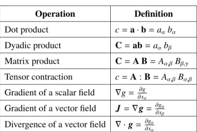
For a clear understanding of the mathematical symbols and equations in this thesis, the notation in use will be shortly announced in this section. If not otherwise stated, vectors are indicated by bold lower-case symbols, e.g.,a and matrices or higher order tensor, respectively, by bold upper-case symbols, likeA. In some cases, where it makes the situation clearer, index notation of vectors or tensors, respectively, is applied. As common in literature, the index notation is used in combination with Einstein’s summation convention. The applied definitions of vector and tensor operations are conform with the standard definitions for Euclidean space, see Table 1.1.
More noteworthy is the description of the Lattice Boltzmann Method. In literature, com-monly all lattice quantities are non-dimensional by the grid spacing ∆x and the time step ∆t, what leads to a spacing∆xl = 1 and a time step∆tl = 1 in lattice units. Since these quantities
un-Table 1.1: Mathematical Definitions Operation Definition Dot product c=a·b= aαbα Dyadic product C=ab=aαbβ Matrix product C=A B= Aα,βBβ,γ Tensor contraction c=A:B= Aα,βBα,β
Gradient of a scalar field ∇g= ∂∂xg
α
Gradient of a vector field J = ∇g= ∂∂gxα β
Divergence of a vector field ∇ · g= ∂gα
∂xα
derstanding and physical interpretation of formulae. In this thesis all quantities and equations of LBM are used in a dimensional description, to circumvent these difficulties and allow an unique interpretation.
Kinetic Theory
The kinetic theory of gases describes a gas on a microscopic or molecular level. As already said in the previous Section 1.3, the condition of the gas could be completely characterized by tracking the position and the velocity of every molecule. Due to the unthinkable large number of molecules in a real gas, this is not feasible and a statistical approach must be used. The introduction to the essential concept given in this section is mainly based on the textbooks by Bird [10] and Hänel [50].
2.1
The Distribution Function
The position of a molecule in physical space can be characterized by its x, yandzcoordinate, which can be combined to a position vector x, see Fig. 2.1(a). A volume element in physical space can be defined bydV = dx·dy·dz. Analog to the physical space, a velocity space can be defined, cf. Fig. 2.1(b). The velocityξof a molecule is a point in the velocity space with the componentsu,vandw. In velocity space a volume element can be expressed bydξ= du·dv·dw. The physical and velocity space are combined to a new six dimensional space called phase space. For the statistical description of the gas a probability distribution function is now defined by:
f(x,ξ,t)= dN
dV ·dξ . (2.1)
The distribution function can be interpreted in two ways:
• Deterministically, as the number of particles dN per phase space volume dV · dξ at a positionxwith a velocityξat a given timet.
x y z x dx dy dz
(a) Physical Space
u v w du dv dw (b) Velocity Space
Figure 2.1: Phase Space
• Statistically, as the possibility to find a molecule in the phase space volumedV ·dξat a positionxwith a velocityξat a given timet.
The distribution function is the central quantity in the kinetic theory of gases, from which all macroscopic quantities can be calculated. This is done by averaging of molecular quantities and is called establishing of moments. A momentMof the distribution function is the integral over the velocity space of a functionφ(ξ), which is either a constant or depending on the molecular velocityξ, multiplied with the distribution function f:
M(x,t)= ∫ ∞ −∞ ∫ ∞ −∞ ∫ ∞ −∞φ (ξ)· f(x,ξ,t)du dv dw B ∫ ξφ (ξ)· f(x,ξ,t)dξ . (2.2)
The definition of the functionφ(ξ) is depending on the macroscopic quantity to determine. Re-ferring to the powernof the molecular velocityξin the functionφ, the corresponding moment is called an-th order moment of the distribution function, e.g., the particle density in Eq. (2.3) is a zeroth order moment. The particle density is established forφ =1, what results in:
n(x,t)= lim dV→0 dN dV = ∫ ξ f(x,ξ,t)dξ . (2.3)
The macroscopic variables, which describe a flow in general are density, pressure, momentum, and temperature. These quantities are recovered by the following moments [50]:
ρ = m· ∫ ξ f(x,ξ,t)dξ (2.4) p = m 3 · ∫ ξ(ξ−u) 2· f(x,ξ,t)dξ (2.5) ρ·u = m· ∫ ξξ· f(x,ξ,t)dξ (2.6) ρ·e= 3 2ρ·R·T = m 2 · ∫ ξ (ξ−u)2· f(x,ξ,t)dξ , (2.7) (2.8)
where m is the molecular mass. Density, pressure, and temperature in the above equations are linked by the equation of state for an ideal gas. Additionally, the macroscopic system of equations, i.e., Navier-Stokes and energy equation, include the momentum flux tensor and the heat flux vector, which are expressible by moments, too:
Π = m· ∫ ξξ ξ· f(x,ξ,t)dξ (2.9) q = m 2 · ∫ ξ|ξ− u|2·(ξ−u)· f(x,ξ,t)dξ . (2.10) For the definition of the remaining, physically interpretable moments the reader is referred to [10, 50].
2.2
The Boltzmann Equation
As shown in the previous section, the knowledge of the distribution function permits the calcu-lation of all macroscopic flow quantities. But, up to now, it is not clear how the distribution function f itself can be determined. Based on the conservation of molecules in a system, which is equal to mass conservation for non reacting molecules, a conditional equation for f, the Boltz-mann equation, can be derived.
The change of the number of moleculesdN in a volume element of the phase spacedV ·dξ
by time, must be related to the following processes (for a more detailed presentation see [10]): • Convective transport of the molecules in and out of the considered physical space volume
dV due to the molecular velocityξ.
• Convective transport of the molecules in and out of the considered velocity space volume
• Gain and loss of molecules in the the considered velocity space volumedξ due to colli-sions of the molecules.
The mathematical formulation of the above principles leads to the Boltzmann equation (see [10] or [50] for a full length derivation):
∂f ∂t +ξ· ∂f ∂x + F m · ∂f ∂ξ = ( ∂f ∂t ) coll . (2.11)
For a better readability the variables of f = f(x,ξ,t) were omitted in Eq. (2.11). The different terms of the Boltzmann equation can now be readily explained: The left-hand side of Eq. (2.11) is called transport or advection term and contains the temporal and the convective change of the distribution function f in physical and velocity space. The right-hand side is referred to as col-lision term and represents the change of the distribution function f due to molecular collisions. For the derivation of the collision term, the assumption of dilute gas is made. This means that the mean free path λ between molecular collisions is much greater than the mean molecular spacingδ, which expresses the mean volume per molecule. δin turn is much greater than the molecular diameterd: λ ≫ δ ≫ d . Consequences of this assumption are that intermolecular forces are negligible and collisions of three or more molecules are very unlikely, so all colli-sions are regarded as binary elastic collicolli-sions between two molecules. As another consequence, the collisions can be considered instantaneous, which means the distribution function does not change during the collision.
The collision term introduced by Boltzmann is presented, for the sake of completeness, in Eq. (2.12). This collision integral is quite complicated and turns the Boltzmann equation into a mathematically difficult to solve integro-differential equation. Equation (2.12) shows the change of the distribution function f = f(x,ξ,t) due to collisions of molecules with speedξand molecules with a different speed ξ1, which are considered in f1 = f1(x,ξ1,t). We see that the
change of f depends on the pre-collision and post-collision (denoted with′) distributions and the relative speedξr= ξ1−ξof the molecules. The collision integral has to be evaluated for all velocitiesξ1 ∈]− ∞,∞[ and the complete differential cross-sectionAc. The reader is referred
to Bird [10] and Hänel [50] for further explanations of Boltzmann’s collision term.
( ∂f ∂t ) coll = ∫ ξ1 ∫ AC (f′ · f1′− f · f1)·ξr dACdξ1 (2.12)
According to classical mechanics, the macroscopic properties mass, momentum, and energy are conserved in elastic collisions. Thus, these quantities are called collisional invariants.
2.3
The Equilibrium Distribution Function
For a physically correct behavior, the Boltzmann equation must satisfy the second law of ther-modynamics. To prove this, Boltzmann defined the H-function and pointed out its relation to
the entropyS [50]: H= ∫ ξ f ln(f)dξ= − 1 kV∆S . (2.13)
He could show from the Boltzmann equation for a homogeneous, closed system that ∂H
∂t ≤0⇔
∂S
∂t ≥0. (2.14)
This proofs the accordance of the Boltzmann equation with the second law of thermodynamics and is known as H-theorem [10, 50].
A quintessence of the H-theorem is that any distribution function f in a homogeneous, closed system will tend with time to a certain distribution function, the equilibrium or Maxwellian distribution. During this process, which is caused by collisions of molecules, the entropy is monotonically increasing up to a finite upper bound, when thermodynamic equilibrium is reached [10, 50].
The distribution function in equilibrium state is mathematically expressed by:
feq = n (2·π·R·T)32 ·exp ( −(ξ−u)2 2·R·T ) . (2.15)
Since the transition to the equilibrium state is generated by collisions, the equilibrium distribu-tion has the same collisional invariants than the primary distribudistribu-tion f.
ρ = m· ∫ ξ f(x,ξ,t)dξ= m· ∫ ξ f eq (x,ξ,t)dξ (2.16) ρ·u = m· ∫ ξξ· f(x,ξ,t)dξ =m· ∫ ξξ· feq(x,ξ,t)dξ (2.17) ρ·e = m 2 · ∫ ξ (ξ−u)2· f(x,ξ,t)dξ= m 2 · ∫ ξ (ξ−u)2· feq(x,ξ,t)dξ (2.18)
2.4
BGK Approximation
The difficulties in the solution of the Boltzmann equation (Eq. (2.11)) are mainly caused by the collision term (Eq. (2.12)). The approximation of the Boltzmann equation after Bhatnagar, Gross and Krook (BGK) [9] uses a simplified collision model. The BGK collision term is defined in the following way:
( ∂f ∂t ) coll =−ω·(f − feq)=−1 τ ·(f − feq). (2.19) The collision process in the BGK approximation is replaced by a relaxation of the distribu-tion funcdistribu-tion f to the local equilibrium feq. The relaxation parameterωis known as collision frequency and defines the time range in which the relaxation occurs. Besides the collision fre-quency, its reciprocal value, the collision timeτ, is often used in literature. Physically seen, this model expresses the consequences of the H-theorem and preserves the collisional invariants.
2.5
The Chapman-Enskog Expansion
By means of the Chapman-Enskog expansion, continuum equations and macroscopic transport coefficients can be derived from the Boltzmann equation. Since this derivation is a tedious mathematical action, the procedure will only be roughly described for the BGK approximation here, according to the approach of [26]. Furthermore, the description is restricted to isothermal flows. Additional presentations of the Chapman-Enskog expansion can be found in [50, 116, 132].
The Chapman-Enskog expansion is a multiscale expansion of the distribution function f and the time t, for small departures from equilibrium, what correlates toKn ≪ 1, i.e., continuum limit. The distribution function f is expanded as a power series inϵ around local equilibrium, where the parameterϵ can be interpreted as the Knudsen number (see also [26, 116, 132]):
f = feq+ϵf1+ϵ2f2+ϵ3f3+... . (2.20)
Analogically, the timetderivative is expanded as power series inϵ as well: ∂ ∂t = ∂ ∂t0 +ϵ∂∂ t1 +... . (2.21)
The timescales in Eq. (2.21) can be interpreted as advective (t0) and viscous (t1) timescales,
according to departure from equilibrium. The next ingredient is to introduce the parameterϵin the collision time τ = ϵτ˜. For convenience, external forces will be neglected in the following. The BGK approximation of the Boltzmann equation reads then as:
∂f ∂t +ξ· ∂f ∂x =− 1 ϵτ˜(f − f eq ). (2.22)
Inserting Eqs. (2.20) and (2.21) in Eq. (2.22) and sorting on the basis ofϵ, brings up forO(1) andO(ϵ): ∂feq ∂t0 +ξ· ∂feq ∂x =− 1 ˜ τf1 (2.23) ϵ ( ∂feq ∂t1 + ∂f1 ∂t0 +ξ· ∂f1 ∂x ) =−ϵ1 ˜ τf2. (2.24)
The zeroth and first order moments of fn, n ≥ 1, are 0 due to collisional invariance. Equation
(2.23) can be interpreted as a zeroth order truncation of theϵexpansion. Establishing the zeroth and first order moments of this equation yields the Euler equations:
∂ρ ∂t0 + ∂ρu ∂x =0 (2.25) ∂ρu ∂t0 + ∂Π∂eq x =0 (2.26)
with: Πeq =m·
∫
ξξ ξ·
feqdξ = pI+ρuu. The zeroth and first order moments of Eq. (2.24) produce:
∂ρ ∂t1 =0 (2.27) ϵ ( ∂ρu ∂t1 + ∂∂Π1 x ) =0. (2.28)
By combination of Eq. (2.25), (2.27), and Eq. (2.26), (2.28), and neglecting terms ofO(ϵ2), the Navier-Stokes equations are recovered. This correlates to a truncation of the power series at first order inϵ. ∂ρ ∂t + ∂ρu ∂x =0 (2.29) ∂ρu ∂t + ∂(Πeq+ϵΠ1) ∂x = 0 (2.30)
The difference between the Euler momentum equations (2.26) and the Navier-Stokes momen-tum equations (2.30) is the friction term, which is expressed by the stress tensor σ = −ϵΠ1. A relation between Π1 and the equilibrium feq can be achieved by building the second order
moment of Eq. (2.23): ∂Πeq ∂t0 + ∂ ∫ ξξξξfeqdξ ∂x =− 1 ˜ τΠ1. (2.31)
The terms on the left hand side of Eq. (2.31) can be expressed in terms of macroscopic quantities [26]: ∂Πeq αβ ∂t0 = ∂∂ t0 ( RTρδαβ+ρuαuβ) (2.32) ∫ ξξαξβξγf eq dξ= ρuαuβuγ+RTρ(uαδβγ +uβδγα+uγδαβ) . (2.33) For incompressible, isothermal flows Eq. (2.31) reduces to [26, 50]:
Π1 αβ = −τ˜RTρ (∂ uβ ∂xα + ∂uα ∂xβ ) . (2.34)
With the continuum definition of the stress tensor [106]
σαβ =µ (∂ uβ ∂xα + ∂uα ∂xβ ) (2.35)
Newton’s Laws ↓ Liouville equation ↓ Boltzmann equation ↓
Navier Stokes equations ↓
Euler equations
Figure 2.2: BBGKY Hierarchy
and Eq. (2.34), a relationship between the collision timeτand the viscosity of the fluid, which is the macroscopic transport coefficient of momentum, can be established. Using the relation σαβ =−ϵΠ1αβone gets:
µ= ϵτρ˜ RT = τρRT = ρRT
ω (2.36)
ν= µρ =τRT = RT
ω . (2.37)
As shown above, the zeroth order truncation of theϵexpansion results in the Euler equations and the first order truncation in the Navier-Stokes equations. Higher order truncations lead to Burnett and super Burnett equations. The derivation of the continuum equations from kinetic equations is part of the BBGKY (Bogoliubov-Born-Green-Kirkwood-Yvon) hierarchy. This hi-erarchy expresses the bottom up approach of describing fluid flows, visualized in Fig. 2.2.
Starting at microscopic level, the motion can be described by Newton’s Laws. Apply-ing kinetic theory, the Liouville equation can be established, which will not be explained here (see [10] for details). The Liouville equation can, under certain assumptions, be transferred to the Boltzmann equation, which itself leads to the Navier-Stokes and Euler equations by the discussed Chapman-Enskog expansion.
The Lattice Boltzmann Method
Historically seen, the Lattice Boltzmann Method emerged from a numerical scheme called Lat-tice Gas Automata as a solver for the Navier-Stokes equations. But, LBM can also be directly derived from the Boltzmann equation. Thus, the Lattice Boltzmann Method is a numerical tech-nique for solving the Boltzmann equation under certain approximations. This derivation and further essential topics of LBM will be shown in the following section. For a detailed illustra-tion of Lattice Gas Automata and the historical development of LBM the reader is referred to the textbooks of Succi [116] and Wolf-Gladrow [132].
In the context of Lattice Boltzmann Methods, the commonly used distribution is slightly different to the definition in Eq. (2.1):
f(x,ξ,t)=m· dN
dV ·dξ (3.1)
The distribution function here includes the molecular mass m compared to Eq. (2.1). This form of distribution is sometimes called density distribution function and will be used in the following.
3.1
The Lattice Boltzmann Equation
Every numerical scheme requires a discretization of the continuous equation and the computa-tional domain. Based on the continuous BGK approximation of the Boltzmann equation (Eqs. (2.11) and (2.19)), a discrete equation, the Lattice Boltzmann equation, is now established.
3.1.1
Discretization of Velocity Space
Velocity space can be discretized by several mathematical methods. Here, the so called discrete velocity method ([1, 10, 110]) is used, since it is intuitive and illustrative. In this method the molecules are restricted to have only a small number of possible velocities, which are discrete values of the velocity space. The calculation of moments according to Eq. (2.2) by integrating over the continuous velocity space must then be converted into a discrete evaluation by a Gauss-Hermite quadrature [52]. M(x,t)= ∫ ∞ −∞φ (ξ)f(x,ξ,t)dξ = q−1 ∑ i=0 φ(ξi)fi (3.2) fi =w˜if(x,ξi,t)) (3.3)
The factors ˜wi and ξi are the weights and nodes or abscissae (i.e. discrete velocities) of the
quadrature. The parameter q is the number of discrete velocities. Possible arrangements of discrete velocities, or quadrature points, respectively, will be discussed in the next section. The identity in Eq. (3.2) implies that the distribution f can be expressed by a polynomial inξ. This can indeed be done by an expansion with a Hermite polynomial, see [110, 111] for details.
The equilibrium distribution function needs discretization as well, to establish their mo-ments in discrete velocity space. The application of the quadrature rules requires the expansion of feq as a polynomial. This can be done by a Taylor series inuof Eq. (2.15), which is
com-monly truncated at second order. (Remember that f is multiplied by the molecular mass in the LBM context.) feq = ρ (2πRT)32 exp ( −ξ2 2RT ) { 1+ (ξ·u) RT + (ξ·u)2 2(RT)2 − u2 2RT } +O(u3) feq = w(ξ)ρ { 1+ (ξ·u) RT + (ξ·u)2 2(RT)2 − u2 2RT } +O(u3) (3.4) The coefficients before the curly brackets in the first presentation of the truncated equilibrium are combined in the weight function w(ξ) in Eq. (3.4). Equation (3.4) can also be seen as a Taylor expansion of the equilibrium in the Mach number (Ma) :
Ma= |u| cs (3.5) cs = √ d p dρ T = √RT (3.6) p ρ =RT . (3.7)
The Mach number is the ratio of the magnitude of the fluid velocity |u|to the speed of sound
cs. The isothermal speed of soundcsfor an ideal gas is given by Eq. (3.6) and the equation of
state for an ideal gas is specified in Eq. (3.7). The truncation of Eq. (3.4) atu2corresponds to a
truncation atMa2and is therefore only valid for small Mach numbers. Fluid flows are generally considered incompressible for small Mach numbers, i.e.,Ma<0.3. This approximation is thus adequate for the restriction made to incompressible, isothermal flows in this thesis.
Moments of the truncated equilibrium distribution, Eq. (3.4), for the discrete velocities ξi result from Eq. (3.2), where fi = w˜ifieq = w˜ifeq(ρ,u,ξi) in this case. Commonly, the discrete
value of the weight functionw(ξi) (Eq. (3.4)) and the value of quadrature weight ˜wi (Eq. 3.3)
are combined to a single weight factorwi, as done in Eq. (3.8).
fieq =w˜iw(ξi)ρ { 1+ (ξi·u) c2 s + (ξi·u)2 2c4 s − u2 2c2 s } fieq = wiρ { 1+ (ξi·u) c2 s + (ξi·u)2 2c4 s − u2 2c2 s } (3.8)
As we can see, the space and time dependence of fieqis only indirect through the space and time dependence ofρ(x,t) andu(x,t).
Since the macroscopic quantities are established from the discrete formulae, the distribution function needs only to be evolved in space and time for the discrete velocitiesξi. In the absence of external forces, the resulting discrete velocity Boltzmann-BGK equation, hereafter called discrete Boltzmann equation, is shown in Eq. (3.9) [1, 110]. The treatment of external forces will be concerned later. Equation (3.9) is a set ofq nonlinear first order differential equations for the discrete values of the distribution function.
∂fi ∂t +ξi· ∂fi ∂x = − 1 τ ·(fi− fieq) (i= 0, ...,q−1) (3.9)
For recovering the isothermal Navier-Stokes equations in the continuum limit, the moments up to second order, i.e., density, momentum, and stress tensor, must be correctly recovered by the discrete model. By applying a Chapman-Enskog expansion to the discrete Boltzmann equation with the discrete equilibrium distribution presented here, it is shown that this model approximates the Navier-Stokes equations with second order accuracy in the Knudsen number
Kn[1].
Another, mathematically very formal way to derive the discrete Boltzmann equation is the expansion of the distribution function with Hermite polynomials. Shan and He [110] show that this approach is equivalent to the discrete velocity method used here. Nevertheless, the expansion by Hermite polynomials yields a direct relation between the truncation order of the polynomial and the representation of the physical system. Equation (3.4) can be interpreted as a second order truncated Hermite polynomial, see [110, 111]. By truncating the Hermite polynomial at higher orders, LBM schemes for simulating thermal and higher Mach number flows can be developed. Higher order truncation means that higher order terms of fluid velocity
or Mach number, respectively, will occur in the discrete equilibrium distribution function and a higher number of Gaussian quadrature pointsξiare needed [111].
3.1.2
Discretization in Space and Time
After discretization in velocity space, the discretization in physical space and time is now per-formed to obtain a model, ready for numerical simulation. The discrete Boltzmann equation can be rewritten with a total or Lagrangian derivative as:
∂fi ∂t +ξi· ∂fi ∂x = D f Dt =− 1 τ ·(fi− fieq). (3.10)
By introducing the convective scaling∆x = ξi∆t, Eq. (3.10) can be integrated along a charac-teristic for a time interval [26, 54]:
∫ ∆t 0 D fi(x+ξis,t+s) Ds ds= ∫ ∆t 0 −1τ[fi(x+ξis,t+s)− f eq i (x+ξis,t+s)]ds. (3.11)
While the total derivative on the left-hand side of Eq. (3.11) integrates directly, the right-hand side needs approximation. Since the discrete Boltzmann equation is second order accurate in terms of Kn, it is reasonable to preserve the order and use a second order accurate quadrature rule. Here the trapezoidal rule is applied:
fi(x+ξi∆t,t+ ∆t)− fi(x,t)=− ∆t 2τ [ fi(x+ξi∆t,t+ ∆t)− f eq i (x+ξi∆t,t+ ∆t) +fi(x,t)− fieq(x,t) ] +O(∆t2). (3.12)
The values of the equilibrium fieq(x+ξi∆t,t+ ∆t) are not known a priory and depend on fi(x+
ξi∆t,t+ ∆t), i∈ {0, ...,q−1}. This creates an implicit system of nonlinear, algebraic equations
from Eq. (3.12). By the following substitution, the system of equations is transformed to a fully explicit system [26, 51, 54]: fi(x,t)= fi(x,t)+ ∆ t 2τ [ fi(x,t)− fieq(x,t) ] . (3.13)
After some algebra one obtains from Eq. (3.12) with (3.13) this explicit set of equations [26, 51, 54]:
fi(x+ξi∆t,t+ ∆t)− fi(x,t)=− ∆t τ+0.5∆t
[
fi(x,t)− fieq(x,t)] . (3.14) The fraction in Eq. (3.14) is from a mathematical point of view a relaxation parameter, which describes relaxation to equilibrium. In analogy to the BGK model, this parameter is considered as a dimensionless collision time, denoted byΩ. Compared to the continuous model, the addi-tional parameter 0.5∆toccurs in the relaxation parameter of the discrete model. This numerical
viscosity, sometimes called discrete lattice effect [47], is absorbed into the physical model, i.e., the relaxation parameter, to obtain correct macroscopic transport coefficients [51]. By using the relationships (2.37) and (3.6),Ωbecomes a function of the kinematic fluid viscosity:
Ω = ∆τt = τ+∆t 0.5∆t = c2s∆t ν+0.5c2 s∆t . (3.15)
Finally the Lattice Boltzmann equation (LBE), sometimes called Lattice BGK equation, is achieved from Eq. (3.16) with the dimensionless collision time. (Note: From Eq. (3.13) it follows fieq = feqi .)
fi(x+ξi∆t,t+ ∆t)= fi(x,t)+ Ω[feqi (x,t)− fi(x,t)] (3.16) The Lattice Boltzmann equation is a set of discrete equations for the evolution of the discrete values of the distribution function fi. The next step is to evaluate the consequences of the substitution process on the macroscopic or hydrodynamic variables. Since fieq = feqi , i.e., the collision operator preserves mass and momentum, the zeroth and first order moments remain unchanged: ρ= q−1 ∑ i=0 fi = q−1 ∑ i=0 ¯ fieq = q−1 ∑ i=0 fieq = q−1 ∑ i=0 fi (3.17) ρu= q−1 ∑ i=0 ξifi = q−1 ∑ i=0 ξif¯ eq i = q−1 ∑ i=0 ξif eq i = q−1 ∑ i=0 ξifi. (3.18)
For the momentum flux tensor things are bit different:
Π = q−1 ∑ i=0 ξiξifi = q−1 ∑ i=0 ξiξifi+ ∆ t 2τ q−1 ∑ i=0 ξiξifi− q−1 ∑ i=0 ξiξif eq i (3.19) = Π+ ∆t 2τ[Π−Π eq]
with : Πneq = Π−Πeq and Πeq =Πeq ⇒Πneq = ( 1+ ∆t 2τ )−1[ Π−Πeq] Πneq = ( 1+ ∆t 2τ )−1∑q−1 i=0 ξiξi ( fi− f eq i ) = ( 1+ ∆t 2τ )−1∑q−1 i=0 ξiξif neq i . (3.20)
Equation (3.20) shows the influence of the discrete lattice effect on the non equilibrium part of the momentum flux tensor. The non equilibrium part of the distribution fineq = fi − fieq is an
approximation for the first order term f1
i of the Chapman-Enskog expansion (cf. Eq. (2.20)).
An important result of the Chapman-Enskog expansion shown above, is the correlation between the macroscopic stress tensor of the Navier-Stokes equations σandΠ1. Using this result and Eqs. (2.37), (3.6), and (3.20) yields an relationship for the macroscopic stress tensor and the momentum flux tensor of the discrete model:
σ = −ϵΠ1 ≈ −Πneq σ = − ( 1+ c 2 s∆t 2ν )−1∑q−1 i=0 ξiξi ( fi− f eq i ) = − ( 2ν 2ν+c2 s∆t )∑q−1 i=0 ξiξi ( fi − f eq i ) = − ( ν ν+0.5c2 s∆t · c2s∆t c2 s∆t )∑q−1 i=0 ξiξi ( fi− f eq i ) σ = − Ων c2 s∆t q−1 ∑ i=0 ξiξi ( fi− f eq i ) (3.21) = − ( 1− 1 2Ω )∑q−1 i=0 ξiξi ( fi− f eq i ) .
The LBE derived here, is a second order accurate discretization of the discrete Boltzmann equation in space and time and, thus, it recovers in the continuum limit the Navier-Stokes equa-tion with second order accuracy. In what follows, only the distribuequa-tion funcequa-tion with an overbar will be used, thus the overbar notation will be omitted for simplicity.
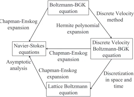
The discretization procedure shown here is not the only way to discretize the discrete Boltz-mann equation in space and time. As demonstrated by Chen and Doolen [21] the time derivative in Eq. (3.9) can be discretized by an Euler forward difference and the convective term by a first order upwind scheme. After introducing the convective scaling∆x = ξi∆t, the Lattice Boltz-mann equation is recovered. But, in contrast to the above derivation, the expression of the relaxation parameter Ω is not derived during the discretization procedure. Instead, it must be determined by a subsequent Chapman-Enskog expansion of the Lattice Boltzmann equation. This procedure reproduces the second order accuracy of LBM to the Navier-Stakes equations as well [51]. Another way to derive the Navier-Stokes equations from the LBE and to show the accuracy of the scheme is the so called asymptotic analysis as proposed by Junk et al. [63]. The different links between the Boltzmann-BGK equation, the discrete Boltzmann equation, and the Navier-Stokes equations are schematically shown up in Fig. 3.1.
Navier-Stokes equations Discrete Velocity Boltzmann-BGK equation Lattice Boltzmann equation Discretization in space and time Chapman-Enskog expansion Chapman-Enskog expansion Asymptotic analysis Boltzmann-BGK equation Chapman-Enskog expansion Discrete Velocity method Hermite polynomial expansion
Figure 3.1: Links to Boltzmann-BGK Equation
3.2
Discrete Phase Space Model
In the preceding section, the Boltzmann equation has been discretized. Therefor, the discrete velocity space was derived by restricting the molecules to certain velocities, which were not clearly specified up to now. The set of discrete velocities must fulfill different requirements.
The most important criteria to meet is Eq. (3.2), which means that the moments of the discrete distribution function are identical to the ones based on the continuous velocity space. But, it can be shown that matching of all moments requires an infinite number of velocities [17]. Since the goal of the discretization is to use only a finite set of velocities, some limitations are needed. Thus, the discrete moments are restricted to be equal to their continuous counterparts up to a certain order m, depending on the physics to be represented. Chen and Shan [17] state that an accurate calculation of the discrete non-equilibrium moment at orderm requires a correct evaluation of the discrete equilibrium moments at order n = m + 1. Furthermore, the accurate calculation of discrete moments defines the degree of precision q ≥ m + n of the Gauss-Hermite quadrature. The precision requirements of the quadrature are equivalent to satisfying the isotropic tensor conditions of Eq. (3.24) by the discrete velocity set [89]. Meeting the isotropic conditions results in rotational invariance of the hydrodynamic moments [20, 46].
Before coming to these isotropic conditions, some definitions are needed: E(n) = q−1 ∑ i=0 wiξ|i ξ{zi... ξ}i n (3.22) Eα(n1),α2,...,αn = q−1 ∑ i=0 wiξi,α1ξi,α2...ξi,αn . (3.23)
The quantityE(n)is a tensor ofn-th order build from the discrete velocitiesξiand the weightswi
(cf. Eq. (3.8)), accordinglyξiξi...ξihas to be understood as a dyadic product. Eα(n1),α2,...,αn can be interpreted as one component of the tensor for fixedα1, α2, ..., αn or by the Einstein convention
as the tensor itself. The indexαj = {x,y,z}expresses a component of the j-th velocity vector in
the tensor product.
E(αn) 1,α2,...,αn = (RT) n/2∆(n) α1,α2,...,αn n= even integer, n≤q 0 n= odd integer, n≤q (3.24)
In the isotropic conditions (Eq. (3.24))∆(αn1),α2,...,αn is then-th order delta function defined as a summation ofn/2 products of Kronecker deltas, see [17] for details.
In what follows, the conditions of Eq. (3.24) will be applied to a set of 19 discrete velocities in a 3 dimensional Cartesian space, commonly named D3Q19 lattice. The notation DdQq goes back to [98], d expresses the dimension of the space and q the number of discrete velocities. The termlatticeis used as a synonym for the discrete phase space or often interchangeable for the discrete velocity space, only. Details about other popular lattices, like D3Q15 and D3Q27 can be found in [46, 85, 98]. The D3Q19 lattice, which is used in SAM-Lattice, is numerically more stable than the D3Q15 lattice and provides a good compromise between accuracy and computational efficiency compared to D3Q15 and D3Q27 [29, 85].
In the D3Q19 lattice, the physical space is discretized by an equally spaced cubic grid. The D3Q19 lattice is shown in Fig. 3.2, including the following 19 discrete velocities:
ξ(0) i =(0,0,0) i= 18 ξ(1) i =(±ξ,˜ 0,0),(0,±ξ,˜ 0),(0,0,±ξ˜) i= 0, ...,5 ξ(2) i =(±ξ,˜ ±ξ,˜ 0),(±ξ,˜ 0,±ξ˜),(0,±ξ,˜ ±ξ˜) i= 6, ...,17 ˜ ξ = ∆∆x t . (3.25)
The velocity vectors originate from every computation node of the cubic grid and end up at the next neighbor in the according direction. They are categorized into three different groups, depending on the length of the vectors. This is usually called energy level. Energy level 0 contains only the zero velocity, molecules with this velocity rest at the current node. The six velocities belonging to energy level 1 point to the next neighbor nodes in Cartesian directions.
ξ0 ξ1 ξ2 ξ3 ξ4 ξ5 ξ6 ξ7 ξ8 ξ9 ξ10 ξ11 ξ12 ξ13 ξ14 ξ15 ξ16 ξ17 1 13 ξ 10 ξ ξ ξ ξ ξ x y z Figure 3.2: D3Q19 Lattice
The left twelve vectors in energy level 2 are chosen to point to the remaining next neighbor nodes, with exception of the space diagonal neighbors. For every discrete velocity, the D3Q19 lattice contains a velocity vector in the opposed direction. This is called parity symmetry. Due to the symmetry of the lattice and the required invariance of the hydrodynamic moments, the weightswi can only be different for the different energy levels, i.e., all velocities in the same
energy level have the same weight [20]. By the definition of the molecular velocity ˜ξ, which was already used for the disrectization of the Boltzmann equation in the previous section, molecules fly exactly from one node to the according neighbor during one time step.
Let us start with the demonstration of Eq. (3.24) for the D3Q19 lattice. A consequence of the parity symmetry of the D3Q19 lattice is, that the tensor of Eq. (3.24) is zero for odd integers. For even integersn∈ {0,2,4}, these three conditions follow [50]:
E(0) = 18 ∑ i=0 wi =1 (3.26) E(2)α 1,α2 = 18 ∑ i=0 wiξi,α1ξi,α2 = RTδα1α2 =c 2 sδα1α2 (3.27) E(4)α 1,α2,α3,α4 = 18 ∑ i=0 wiξi,α1ξi,α2ξi,α3ξi,α4 = RT2(δα1α2δα3α4 +δα1α3δα2α4 +δα1α4δα2α2 ) = c4s(δα1α2δα3α4+δα1α3δα2α4 +δα1α4δα2α2 ) . (3.28)
The solution of Eqs. (3.26) - (3.28) yields to the ratio of the molecular velocity to the speed of sound and to the weights for the three different energy levels:
˜ ξ cs = √3 (3.29) wi = 1 3 i=18 wi = 1 18 i=0, ...,5 wi = 1 36 i=6, ...,17. (3.30)
As said before, modeling of incompressible, isothermal flows requires the correct establish-ing of moments up to second order, i.e., m = 2. Consequently, the equilibrium moments up to ordern = 3 must be correctly evaluated in the discrete model. Nie et al. [89] show that the correct calculation of the third order equilibrium moment, which is the equilibrium heat flux vector, requires in general at least 39 velocity directions in 3D and a third order expansion of
fieq. This is not fulfilled by the D3Q19 lattice and leads to a non Galilean invariant viscous stress [28, 89]. The error in the viscous stress is ofO(Ma3) [28] and thus negligible for small
Ma, i.e., incompressible flow, what is also turned out by the numerical investigation of [89]. In practice, the Galilean invariant D3Q39 lattice or models with even more velocities are hardly used, due to the considerable higher computational costs and memory demands.
With the quantities derived in this section, the discrete model is completely described. In the numerical scheme, the Lattice Boltzmann equation (3.16) is solved every time step, at ev-ery computation node for evev-ery discrete velocity. The remaining parts of this section introduce further basic ingredients of the numerical scheme.
3.3
Collision Operators
Besides the BGK model introduced in detail before, different other collision operators are in use for Lattice Boltzmann methods. In this section we will present the multiple relaxation time model (MRT), which is used in SAM-Lattice in detail. Other collision models, like the entropic [6] or cascaded [43] models will not be discussed here because they are currently not implemented in SAM-Lattice. The interested reader is referred to the mentioned literature.
3.3.1
Single Relaxation Time Model
The term single relaxation time model (SRT) is often used as a synonym for the classical BGK model. In the BGK model, a single relaxation parameterΩ (see Eq. (3.16)) is used for relax-ation to equilibrium. Thus, all physical processes are relaxed with the same rate or time scale,