Min-Max Approximate Dynamic Programming
Brendan O’Donoghue
Yang Wang
Stephen Boyd
Abstract— In this paper we describe an approximate dynamic programming policy for a discrete-time dynamical system perturbed by noise. The approximate value function is the pointwise supremum of a family of lower bounds on the value function of the stochastic control problem; evaluating the control policy involves the solution of a min-max or saddle-point problem. For a quadratically constrained linear quadratic control problem, evaluating the policy amounts to solving a semidefinite program at each time step. By evaluating the policy, we obtain a lower bound on the value function, which can be used to evaluate performance: When the lower bound and the achieved performance of the policy are close, we can conclude that the policy is nearly optimal. We describe several numerical examples where this is indeed the case.
I. INTRODUCTION
We consider an infinite horizon stochastic control problem with discounted objective and full state infor-mation. In the general case this problem is difficult to solve, but exact solutions can be found for certain special cases. When the state and action spaces are finite, for example, the problem is readily solved. Another case for which the problem can be solved exactly is when the state and action spaces are finite dimensional real vector spaces, the system dynamics are linear, the cost function is convex quadratic, and there are no constraints on the action or the state. In this case optimal control policy is affine in the state variable, with coefficients that are readily computable [1], [2], [3], [4].
One general method for finding the optimal policy is to use dynamic programming (DP). DP represents the optimal policy in terms of an optimization problem involving the value function of the stochastic control problem [3], [4], [5]. However, due to the ‘curse of di-mensionality’, even representing the value function can be intractable when the state or action spaces are infinite, or as a practical matter, when the number of states or actions is very large. Even when the value function can be represented, evaluating the optimal policy can still be intractable. As a result approximate dynamic programming (ADP) has been developed as a general method for finding suboptimal control policies [6], [7], [8]. In ADP we substitute an approximate value function for the value function in the expression for the optimal policy. The goal is to choose the approximate value
function (also known as a control-Lyapunov function) so that the performance of the resulting policy is close to optimal, or at least, good.
In this paper we develop a control policy which we call the min-max approximate dynamic programming policy. We first parameterize a family of lower bounds on the true value function; then we perform control, taking the pointwise supremum over this family as our approximate value function. The condition we use to parameterize our family of bounds is related to the ‘linear programming approach’ to ADP, which was first introduced in [9], and extended to approximate dynamic programming in [10], [11]. The basic idea is that any function which satisfies the Bellman inequality is a lower bound on the true value function [3], [4].
It was shown in [12] that a better lower bound can be attained via an iterated chain of Bellman inequalities, which we use here. We relate this chain of inequalities to a forward look-ahead in time, in a similar sense to that of model predictive control (MPC) [13], [14]. Indeed many types of MPC can be thought of as performing min-max ADP with a particular (generally affine) family of underestimator functions.
In cases where we have a finite number of states and inputs, evaluating our policy requires solving a linear program at every time step. For problems with an infinite number of states and inputs, the method requires the solution of a semi-infinite linear program, with a finite number of variables, but an infinite number of constraints (one for every state-control pair). For these problems we can obtain a tractable semidefinite program (SDP) approximation using methods such as the S -procedure [8], [12]. Evaluating our policy then requires solving an SDP at each time step [15], [16].
Much progress has been made in solving structured convex programs efficiently (see, e.g., [17], [18], [19], [20]). These fast optimization methods make our policies practical, even for large problems, or those requiring fast sampling rates.
II. STOCHASTIC CONTROL
Consider a discrete time-invariant dynamical system, with dynamics described by
xt+1=f(xt, ut, wt), t= 0,1, . . . , (1) 2011 IEEE International Symposium on Computer-Aided Control System Design (CACSD)
Part of 2011 IEEE Multi-Conference on Systems and Control Denver, CO, USA. September 28-30, 2011
where xt ∈ X is the system state, ut ∈ U is the control input or action,wt∈ W is an exogenous noise or disturbance, at time t, and f : X × U × W → X is the state transition function. The noise terms wt are independent identically distributed (IID), with known distribution. The initial state x0 is also random
with known distribution, and is independent ofwt. We consider causal, time-invariant state feedback control policies
ut=φ(xt), t= 0,1, . . . ,
whereφ:X → U is thecontrol policyorstate feedback function.
The stage cost is given by ℓ:X × U →R∪ {+∞}, where the infinite values ofℓencode constraints on the states and inputs: The state-action constraint set C ⊂ X × U is C={(z, v)|ℓ(z, v)<∞}. (The problem is unconstrained ifC=X × U.)
Thestochastic control problemis to chooseφin order to minimize the infinite horizon discounted cost
Jφ=E ∞ X t=0 γtℓ(x t, φ(xt)), (2)
whereγ ∈(0,1)is a discount factor. The expectations are over the noise terms wt, t = 0,1, . . ., and the initial statex0. We assume here that the expectation and
limits exist, which is the case under various technical assumptions [3], [4]. We denote byJ⋆
the optimal value of the stochastic control problem,i.e., the infimum ofJφ over all policiesφ:X → U.
A. Dynamic programming
In this section we briefly review the dynamic pro-gramming characterization of the solution to the stochas-tic control problem. For more details, see [3], [4].
Thevalue functionof the stochastic control problem, V⋆:X →R∪ {∞}, is given by V⋆(z) = inf φ E ∞ X t=0 γtℓ(x t, φ(xt)) ! ,
subject to the dynamics (1) and x0 = z; the infimum
is over all policies φ : X → U, and the expectation is over wt for t = 0,1, . . .. The quantity V⋆(z) is the cost incurred by an optimal policy, when the system is started from state z. The optimal total discounted cost is given by
J⋆=E x0
V⋆(x 0).
It can be shown that the value function is the unique fixed point of the Bellman equation
V⋆(z) = inf v ℓ(z, v) +γE wV ⋆(f(z, v, w)
for allz∈ X. We can write the Bellman equation in the form
V⋆=TV⋆,
(3) where we define the Bellman operatorT as
(Tg)(z) = inf v ℓ(z, v) +γE wg(f(z, v, w)) for anyg:X →R∪ {+∞}.
An optimal policy for the stochastic control problem is given by φ⋆(z) = argmin v ℓ(z, v) +γE wV ⋆(f(z, v, w)), (4) for allz∈ X.
B. Approximate dynamic programming
In many cases of interest, it is intractable to compute (or even represent) the value function V⋆, let alone carry out the minimization required evaluate the optimal policy (4). In such cases, a common alternative is to replace the value function with an approximate value functionVˆ [6], [7], [8]. The resulting policy, given by
ˆ φ(z) = argmin v ℓ(z, v) +γE w ˆ V(f(z, v, w)),
for all z ∈ X, is called an approximate dynamic programming (ADP) policy. Clearly, when Vˆ = V⋆, the ADP policy is optimal. The goal of approximate dynamic programming is to find aVˆ for which the ADP policy can be easily evaluated (for instance, by solving a convex optimization problem), and also attains near-optimal performance.
III. MIN-MAX APPROXIMATE DYNAMIC PROGRAMMING
We consider a family of linearly parameterized (can-didate) value functionsVα:X →R,
Vα= K
X
i=1
αiV(i),
where α ∈ RK is a vector of coefficients and V(i) : X →Rare fixed basis functions. Now suppose we have a setA ⊂RK for which
Vα(z)≤V⋆(z), ∀z∈ X, ∀α∈ A.
Thus {Vα | α ∈ A} is a parameterized family of underestimators of the value function. (We will discuss how to obtain such a family later.) For anyα∈ A we have
Vα(z)≤sup α∈A
i.e., the pointwise supremum over the family of under-estimators must be at least as good an approximation of V⋆
as any single function from the family. This suggests the ADP control policy
˜ φ(z) = argmin v ℓ(z, v) +γE wαsup∈AVα(f(z, v, w)) , where we use supα∈AVα(z) as an approximate value function. Unfortunately, this policy may be diffi-cult to evaluate, since evaluating the expectation of the supremum can be hard, even when evaluating
EVα(f(z, v, w))for a particularαcan be done. Our last step is to exchange expectation and supre-mum to obtain themin-max control policy
φmm(z) = argmin
vsupα∈A(ℓ(z, v)
+γEwVα(f(z, v, w))) (5) for all z ∈ X. Computing this policy involves the solution of a min-max or saddle-point problem, which we will see is tractable in certain cases. One such case is where the functionℓ(z, v)+EwVα(f(z, v, w))is convex inv for eachz andαand the setAis convex. A. Bounds
The optimal value of the optimization problem in the min-max policy (5) is a lower on the value function at every state. To see this we note that
infvsupα∈A
ℓ(z, v) +γEVα(f(z, u, w)) ≤infv ℓ(z, v) +γEsupα∈AVα(f(z, u, w)) ≤infv ℓ(z, v) +γEV⋆(f(z, u, w)) = (TV⋆)(z) =V⋆(z),
where the first inequality is due to Fatou’s lemma [21], the second inequality follows from the monotonicity of expectation, and the equality comes from the fact that V⋆
is the unique fixed point of the Bellman operator. Using the pointwise bounds, we can evaluate a lower bound on the optimal costJ⋆ via Monte Carlo simula-tion: Jlb= (1/N) N X j=1 Vlb(zj)
wherez1, . . . , zN are drawn from the same distribution as x0 and Vlb(zj) is the lower bound we get from evaluating the min-max policy atzj.
The performance of the min-max policy can also be evaluated using Monte Carlo simulation, and provides an
upper boundJub on the optimal cost. Ignoring Monte
Carlo error we have
Jlb≤J⋆≤Jub.
Theses upper and lower bounds on the optimal value of the stochastic control problem are readily evaluated numerically, through simulation of the min-max control policy. WhenJlb andJub are close, we can conclude
that the min-max policy is almost optimal. We will use this technique to evaluate the performance of the min-max policy for our numerical examples.
B. Evaluating the min-max control policy
Evaluating the min-max control policy often requires exchanging the order of minimization and maximization. For any functionf :Rp×Rq →Rand setsW ⊆ Rp,
Z ⊆Rq, the max-min inequalitystates that sup
z∈Z inf
w∈Wf(w, z)≤winf∈Wzsup∈Zf(w, z). (6)
In the context of the min-max control policy, this means we can swap the order of minimization and maximization in (5) and maintain the lower bound prop-erty. To evaluate the policy, we solve the optimization problem
maximize infv(ℓ(z, v) +γEwVα(f(z, v, w))) subject to α∈ A
(7) with variable α. If A is a convex set, (7) is a convex optimization problem, since the objective is the infimum over a family of affine functions inα, and is therefore concave. In practice, solving (7) is often much easier than evaluating the min-max control policy directly.
In addition, if there existw˜ ∈ Wandz˜∈ Zsuch that f( ˜w, z)≤f( ˜w,z)˜ ≤f(w,z),˜
for allw∈ Wandz∈ Z, then we have thestrong max-min property (or saddle-point property) and (6) holds with equality. In such cases the problems (5) and (7) are equivalent, and we can use Newton’s method or duality considerations to solve (5) or (7) [16], [22].
IV. ITERATEDBELLMAN INEQUALITIES In this section we describe how to parameterize a family of underestimators of the true value function. The idea is based on the Bellman inequality, [10], [8], [12], and results in a convex condition on the coefficientsα that guaranteesVα≤V⋆.
A. Basic Bellman inequality
The basic condition works as follows. Suppose we have a functionV :X →R, which satisfies the Bellman inequality
V ≤ TV. (8)
Then by the monotonicity of the Bellman operator, we have
V ≤ lim k→∞T
kV =V⋆,
so any function that satisfies the Bellman inequality must be a value function underestimator. Applying this condition toVα and expanding (8) we get
Vα(z)≤inf v ℓ(z, v) +γE wVα(f(z, v, w)) , for all z ∈ X. For each z, the left hand side is linear in α, and the right hand side is a concave function of α, since it is the infimum over a family of affine functions. Hence, the Bellman inequality leads to a convex constraint onα.
B. Iterated Bellman inequalities
We can obtain better (i.e., larger) lower bounds on the value function by considering an iterated form of the Bellman inequality [12]. Suppose we have a sequence of functions Vi :X → R, i= 0, . . . , M, that satisfy a chain of Bellman inequalities
V0≤ TV1, V1≤ TV2, . . . VM−1≤ TVM, (9) with VM−1 = VM. Then, using similar arguments as before we can showV0≤V⋆. Restricting each function
to lie in the same subspace Vi=
K
X
j=1
αijV(j),
we see that the iterated chain of Bellman inequalities also results in a convex constraint on the coefficients αij. Hence the condition on α0j,j = 1, . . . , K, which parameterizes our underestimator V0, is convex. It is
easy to see that the iterated Bellman condition must give bounds that are at least as good as the basic Bellman inequality, since any function that satisfies (8) must be feasible for (9) [12].
V. BOX CONSTRAINED LINEAR QUADRATIC CONTROL
This section follows a similar example presented in [12]. We haveX =Rn,U =Rm, with linear dynamics
xt+1=Axt+But+wt,
whereA∈Rn×n andB ∈Rn×m. The noise has zero mean, Ewt = 0, and covariance EwtwTt = W. (Our
bounds and policy will only depend on the first and second moments ofwt.) The stage cost is given by
ℓ(z, v) = vTRv+zTQz, kvk ∞≤1 +∞, kvk∞>1, whereR=RT 0 ,Q=QT 0 . A. Iterated Bellman inequalities
We look for convex quadratic approximate value functions
Vi(z) =zTPiz+ 2pTiz+si, i= 0, . . . , M,
where Pi = PiT 0, pi ∈ Rn and ri ∈ R, are the coefficients of our linear parameterization. The iterated Bellman inequalities are
Vi−1(z)≤ℓ(z, v) +γEVi(Az+Bv+w),
for allkvk∞≤1,z∈Rn,i= 1, . . . , M. Defining
Si= 0 0 0 0 Pi pi 0 pT i si , L= R 0 0 0 Q 0 0 0 0 , Gi= BTP iB BTPiA BTpi ATP iB ATPiA ATpi pT i B p T i A Tr(PiW) +si ,
fori= 0, . . . , M, we can write the Bellman inequalities as a quadratic form in(v, z,1) v z 1 T (L+γGi−Si−1) v z 1 ≥0, (10) for allkvk∞≤1,z∈Rn,i= 1, . . . , M.
We will obtain a tractable sufficient condition for this using theS-procedure [15], [12]. The constraintkvk∞≤ 1 can be written in terms of quadratic inequalities
1−vT(eieTi )v≥0, i= 1, . . . , m,
where ei denotes the ith unit vector. Using the S -procedure, a sufficient condition for (10) is the existence of diagonal matricesDi0,i= 1, . . . , M for which
L+γGi−Si−1+ Λi0, i= 1, . . . M, (11) where Λi= Di 0 0 0 0 0 0 0 −Tr(Di) . (12)
B. Min-max control policy
For this problem, it is easy to show that the strong max-min property holds, and therefore problems (5) and (7) are equivalent. To evaluate the min-max control policy we solve problem (7), which we can write as
maximize infv(ℓ(z, v) +γEwV0(Az+Bv+w))
subject to (11), SM−1=SM, P00
Pi0, Di0, i= 1, . . . , M, with variables Pi, pi, si, i = 0, . . . , M, and diagonal Di, i = 1, . . . , M. We will convert this max-min problem to a max-max problem by forming the dual of the minimization part. Introducing a diagonal matrix D00as the dual variable for the box constraints, we
obtain the dual function inf v v z 1 T (L+γG0−Λ0) v z 1 ,
whereΛ0 has the form given in (12). We can minimize
overvanalytically. If we block out the matrixL+γG0−
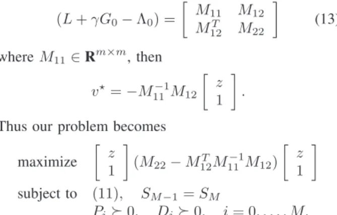
Λ0 as (L+γG0−Λ0) = M11 M12 MT 12 M22 (13) whereM11∈Rm ×m , then v⋆=−M−1 11 M12 z 1 . Thus our problem becomes
maximize z 1 (M22−M12TM −1 11 M12) z 1 subject to (11), SM−1=SM Pi0, Di0, i= 0, . . . , M, which is a convex optimization problem in the variables Pi,pi,ri, Di, i= 0, . . . , M, and can be solved as an SDP.
To implement the min-max control policy, at each timet, we solve the above problem withz=xt, and let
ut=−M⋆ −1 11 M12⋆ xt 1 , whereM⋆
11andM12⋆ denote the matricesM11andM12,
computed fromP⋆
0,p⋆0,s⋆0,D0⋆.
C. Interpretations
We can easily verify that the dual of the above optimization problem is a variant of model predictive control, that uses both the first and second moments of the state. In this context, the number of iterations,M, is the length of the prediction horizon, and we can interpret
Policy / Bound Value MPC policy 1.3147 Min-max policy 1.3145 Lower bound 1.3017
TABLE I:Performance comparison, box constrained example.
our lower bound as a finite horizon approximation to an infinite horizon problem, which underestimates the optimal infinite horizon cost. TheS-procedure relaxation also has a natural interpretation: in [23], the author obtains similar LMIs by relaxing almost sure constraints into constraints that are only required to hold in expec-tation.
D. Numerical instance
We consider a numerical example with n= 8,m= 3, and γ = 0.9. The parameters Q, R, A and B are randomly generated; we setkBk= 1and scaleAso that max|λi(A)|= 1(i.e., so that the system is marginally stable). The initial statex0is Gaussian, with zero mean.
Table I shows the performance of the min-max policy and certainty equivalent MPC, both with horizons of M = 15steps, as well as the lower bound on the optimal cost. In this case, both the min-max policy and MPC are no more than around1%suboptimal, modulo Monte Carlo error.
VI. DYNAMIC PORTFOLIO OPTIMIZATION In this example, we manage a portfolio of n assets over time. Our state xt ∈ Rn is the vector of dollar values of the assets, at the beginning of investment period t. Our action ut ∈ Rn represents buying or selling assets at the beginning of each investment period: (ut)i>0 means we are buying asseti, for dollar value (ut)i, (ut)i <0 means we sell asset i. The post-trade portfolio is then given byxt+ut, and the total gross cash put in is1Tu
t, where1is the vector with all components one.
The portfolio propagates over time (i.e., over the investment period) according to
xt+1 =At(xt+ut)
whereAt=diag(ρt), and(ρt)i is the (total) return of assetiin investment periodt. The return vectorsρtare IID, with first and second moments
(Here too, our bounds and policy will only depend on the first and second moments ofρt.) We let Σ = Σˆ −µµT denote the return covariance.
We now describe the constraints and objective. We constrain the risk of our post-trade portfolio, which we quantify as the portfolio return variance over the period:
(xt+ut)TΣ(xˆ t+ut)≤l,
where l ≥ 0 is the maximum variance (risk) allowed. Our action (buying and selling) ut incurs a transaction cost with an absolute value and a quadratic component, given by κT|u|+uTRu, where κ ∈ Rn
+ is the vector
of linear transaction cost rates (and|u|means element-wise), andR ∈Rn×n, which is diagonal with positive entries, represents a quadratic transaction cost coeffi-cients. (Linear transactions cost model effects such as crossing the bid-ask spread, while quadratic transaction costs model effects such as price-impact.) Thus at time t, we put into our portfolio the net cash amount
g(ut) =1Tut+κT|ut|+uTtRut.
(When this is negative, it represents revenue.) The first term is the gross cash in from purchases and sales; the second and third terms are the transaction fees. The stage cost, including the risk limit, is
ℓ(z, v) =
(
g(v), (z+v)TΣ(zˆ +v)≤l +∞, otherwise.
Our goal is to minimize the discounted cost (or equiv-alently, to maximize the discounted revenue). In this example, the discount factor has a natural interpretation as reflecting the time value of money.
A. Iterated Bellman Inequalities
We incorporate another variable,y ∈Rn, to remove the absolute value term from the stage cost function, and add the constraints
−(yt)i≤(vt)i≤(yt)i, i= 1, . . . , n. (14) We define the stage cost with these new variables to be ℓ(z, v, y) =1Tv+κTy+ (1/2)vTRv+ (1/2)yTRy for(z, v, y)that satisfy
−y≤v≤y, (z+v) ˆΣ(z+v)≤l, (15) and+∞otherwise. Here, the first set of inequalities is interpreted elementwise.
We look for convex quadratic candidate value func-tions,i.e.
Vi(z) =zTPiz+ 2pTiz+si, i= 0, . . . , M,
wherePi 0,pi ∈Rn, si ∈Rare the coefficients of our linear parameterization. Defining
L= R/2 0 0 1/2 0 R/2 0 κ/2 0 0 0 0 1T/2 κT/2 0 0 , Gi= Pi◦Σ 0 Pi◦Σ pi◦µ 0 0 0 0 Pi◦Σ 0 Pi◦Σ pi◦µ (pi◦µ)T 0 (pi◦µ)T 0 , Si = 0 0 0 0 0 0 0 0 0 0 Pi pi 0 0 pT i si , i= 0, . . . , M,
where ◦ denotes the Hadamard product, we can write the iterated Bellman inequalities as
v y z 1 T (L+γGi−Si−1) v y z 1 ≥0,
for all(v, y, z)that satisfy (15), fori= 1, . . . , M. A tractable sufficient condition for the Bellman in-equalities is (by theS-procedure) the existence ofλi≥ 0,νi∈Rn+,τi∈Rn+,i= 1, . . . , M such that L+γGi−Si−1+ Λi0, i= 1, . . . , M, (16) where Λi= λiΣˆ 0 λiΣˆ νi−τi 0 0 0 νi+τi λiΣˆ 0 λiΣˆ 0 νT i −τ T i ν T i +τ T i 0 −λil . (17)
Lastly we have the terminal constraint,SM−1=SM. B. Min-max control policy
The discussion here follows almost exactly the one presented for the previous example. It is easy to show that in this case we have the strong max-min property. At each step, we solve problem (7) by converting the max-min problem into a max-max problem, using Lagrangian duality. We can write problem (7) as
maximize infv,y(ℓ(z, v, y) +γEρV0(A(z+v)))
subject to (16), SM−1=SM Pi0, i= 0, . . . , M,
with variables Pi,pi,si, i= 0, . . . , M, and λi ∈ R+,
νi ∈Rn+,τi∈Rn+,i= 1, . . . , M.
Next, we derive the dual function of the minimization part. We introduce variables λ0 ∈ R+, ν0 ∈ Rn+,
τ0∈Rn+, which are dual variables corresponding to the
constraints (15) and (14). The dual function is given by
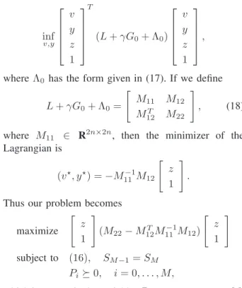
inf v,y v y z 1 T (L+γG0+ Λ0) v y z 1 ,
whereΛ0 has the form given in (17). If we define
L+γG0+ Λ0= " M11 M12 MT 12 M22 # , (18) where M11 ∈ R2n ×2n
, then the minimizer of the Lagrangian is (v⋆, y⋆) =−M−1 11 M12 " z 1 # . Thus our problem becomes
maximize " z 1 # (M22−M12TM −1 11 M12) " z 1 # subject to (16), SM−1=SM Pi 0, i= 0, . . . , M,
which is convex in the variablesPi,pi,si,i= 0, . . . , M, andλi ∈R+,νi∈R+n,τi∈Rn+,i= 0, . . . , M.
To implement the policy, at each timetwe solve the above optimization problem (as an SDP) with z =xt, and let ut=− h Im 0 i M⋆−1 11 M ⋆ 12 " xt 1 # , whereM⋆
11andM12⋆ denote the matricesM11andM12,
computed fromP⋆
0,p⋆0,s⋆0,λ⋆0,ν0⋆,τ0⋆.
C. Numerical instance
We consider a numerical example with n= 8assets andγ= 0.96. The initial portfoliox0is Gaussian, with
zero mean. The returns follow a log-normal distribution, i.e., log(ρt) ∼ N(˜µ,Σ)˜ . The parameters µ and Σ are given by
µi= exp(˜µi+ ˜Σii/2), Σij =µiµjexp( ˜Σij). Table II compares the performance of the min-max policy forM = 40andM = 5, and certainty equivalent model predictive control with horizon T = 40, over 1150 simulations each consisting of 150 time steps. We
can see that the min-max policy significantly outper-forms MPC, which actually makes a loss on average (since the average cost is positive). The cost achieved by the min-max policy is close to the lower bound, which shows that both the policy and the bound are nearly optimal. In fact, the gap is small even forM = 5, which corresponds to a relatively myopic policy.
Bound / Policy Value MPC policy,T = 40 25.4 Min-max policy,M = 5 -224.1 Min-max policy,M = 40 -225.1 Lower bound,M = 40 -239.9 Lower bound,M = 5 -242.0
TABLE II:Performance comparison, portfolio example.
VII. CONCLUSIONS
In this paper we introduce a control policy which we refer to asmin-max approximate dynamic programming. Evaluating this policy at each time step requires the solution of a min-max or saddle point problem; in addition, we obtain a lower bound on the value function, which can used to estimate (via Monte Carlo simulation) the optimal value of the stochastic control problem.
We demonstrate the method with two examples, where the policy can be evaluated by solving a convex opti-mization problem at each time-step. In both examples the lower bound and the achieved performance are very close, certifying that the min-max policy is very close to optimal.
REFERENCES
[1] R. Kalman, “When is a linear control system optimal?”Journal of Basic Engineering, vol. 86, no. 1, pp. 1–10, 1964.
[2] S. Boyd and C. Barratt, Linear controller design: Limits of performance. Prentice-Hall, 1991.
[3] D. Bertsekas, Dynamic Programming and Optimal Control: Volume 1. Athena Scientific, 2005.
[4] ——,Dynamic Programming and Optimal Control: Volume 2. Athena Scientific, 2007.
[5] D. Bertsekas and S. Shreve, Stochastic optimal control: The discrete-time case. Athena Scientific, 1996.
[6] D. Bertsekas and J. Tsitsiklis, Neuro-Dynamic Programming, 1st ed. Athena Scientific, 1996.
[7] W. Powell, Approximate dynamic programming: solving the curses of dimensionality. John Wiley & Sons, Inc., 2007. [8] Y. Wang and S. Boyd, “Performance bounds for linear stochastic
control,”Systems & Control Letters, vol. 58, no. 3, pp. 178–182, Mar. 2009.
[9] A. Manne, “Linear programming and sequential decisions,”
Management Science, vol. 6, no. 3, pp. 259–267, 1960. [10] D. De Farias and B. Van Roy, “The linear programming approach
to approximate dynamic programming,” Operations Research, vol. 51, no. 6, pp. 850–865, 2003.
[11] P. Schweitzer and A. Seidmann, “Generalized polynomial ap-proximations in markovian decision process,”Journal of mathe-matical analysis and applications, vol. 110, no. 2, pp. 568–582, 1985.
[12] Y. Wang and S. Boyd, “Approximate dynamic programming via iterated bellman inequalities,” 2010, manuscript.
[13] C. Garcia, D. Prett, and M. Morari, “Model predictive control: theory and practice,” Automatica, vol. 25, no. 3, pp. 335–348, 1989.
[14] J. Maciejowski,Predictive Control with Constraints. Prentice-Hall, 2002.
[15] S. Boyd, L. E. Ghaoui, E. Feron, and V. Balakrishnan,Linear Matrix Inequalities in System and Control Theory. Society for Industrial Mathematics, 1994.
[16] S. Boyd and L. Vandenberghe,Convex optimization. Cambridge University Press, Sept. 2004.
[17] Y. Wang and S. Boyd, “Fast model predictive control using online optimization,” IEEE Transactions on Control Systems Technology, vol. 18, pp. 267–278, 2010.
[18] ——, “Fast evaluation of quadratic control-lyapunov policy,”
IEEE Transactions on Control Systems Technology, pp. 1–8, 2010.
[19] J. Mattingley, Y. Wang, and S. Boyd, “Code generation for receding horizon control,” inIEEE Multi-Conference on Systems and Control, 2010, pp. 985–992.
[20] J. Mattingley and S. Boyd, “CVXGEN: A code generator for embedded convex optimization,” 2010, manuscript.
[21] D. Cohn,Measure Theory. Birkh¨auser, 1997.
[22] A. Ben-Tal, L. E. Ghaoui, and A. Nemirovski,Robust optimiza-tion. Princeton University Press, 2009.
[23] A. Gattami, “Generalized linear quadratic control theory,” Pro-ceedings of the 45th IEEE Conference on Decision and Control, pp. 1510–1514, 2006.