Out-of-Sample Forecast Tests Robust to the Choice of
Window Size
Barbara Rossi
and
Atsushi Inoue
(
ICREA,UPF,CREI,BGSE,Duke) (NC State)
April 1, 2012
Abstract
This paper proposes new methodologies for evaluating out-of-sample forecasting performance that are robust to the choice of the estimation window size. The method-ologies involve evaluating the predictive ability of forecasting models over a wide range of window sizes. We show that the tests proposed in the literature may lack the power to detect predictive ability and might be subject to data snooping across di¤erent window sizes if used repeatedly. An empirical application shows the usefulness of the methodologies for evaluating exchange rate models’forecasting ability.
Keywords: Predictive Ability Testing, Forecast Evaluation, Estimation Window.
Acknowledgments: We thank the editor, the associate editor, two referees as well as S. Burke, M.W. McCracken, J. Nason, A. Patton, K. Sill, D. Thornton and seminar par-ticipants at the 2010 Econometrics Workshop at the St. Louis Fed, Bocconi University, U. of Arizona, Pompeu Fabra U., Michigan State U., the 2010 Triangle Econometrics Conference, the 2011 SNDE Conference, the 2011 Conference in honor of Hal White, the 2011 NBER Summer Institute and the 2011 Joint Statistical Meetings for useful comments and suggestions. This research was supported by National Science Founda-tion grants SES-1022125 and SES-1022159 and North Carolina Agricultural Research Service Project NC02265.
1
Introduction
This paper proposes new methodologies for evaluating the out-of-sample forecasting perfor-mance of economic models. The novelty of the methodologies that we propose is that they are robust to the choice of the estimation and evaluation window size. The choice of the estimation window size has always been a concern for practitioners, since the use of di¤er-ent window sizes may lead to di¤erdi¤er-ent empirical results in practice. In addition, arbitrary choices of window sizes have consequences about how the sample is split into in-sample and out-of-sample portions. Notwithstanding the importance of the problem, no satisfactory solution has been proposed so far, and in the forecasting literature it is common to only report empirical results for one window size. For example, to illustrate the di¤erences in the window sizes, we draw on the literature on forecasting exchange rates (the empirical application we will focus on): Meese and Rogo¤ (1983a) use a window of 93 observations in monthly data, Chinn (1991) a window size equal to 45 in quarterly data, Qi and Wu (2003) use a window of 216 observations in monthly data, Cheung et al. (2005) consider windows of 42 and 59 observations in quarterly data, Clark and West’s (2007) window is 120 observations in monthly data, Gourinchas and Rey (2007) consider a window of 104 obser-vations in quarterly data, and Molodtsova and Papell (2009) consider a window size of 120 observations in monthly data. This common practice raises two concerns. A …rst concern is that the “ad hoc” window size used by the researcher may not detect signi…cant predic-tive ability even if there would be signi…cant predicpredic-tive ability for some other window size choices. A second concern is the possibility that satisfactory results were obtained simply by chance, after data snooping over window sizes. That is, the successful evidence in favor of predictive ability might have been found after trying many window sizes, although only the results for the successful window size were reported and the search process was not taken into account when evaluating their statistical signi…cance. Only rarely do researchers check the robustness of the empirical results to the choice of the window size by reporting results for a selected choice of window sizes. Ultimately, however, the size of the estimation window is not a parameter of interest for the researcher: the objective is rather to test predictive ability and, ideally, researchers would like to reach empirical conclusions that are robust to the choice of the estimation window size.
This paper views the estimation window as a “nuisance parameter”: we are not interested in selecting the “best” window; rather we would like to propose predictive ability tests that are “robust” to the choice of the estimation window size. The procedures that we
propose ensure that this is the case by evaluating the models’ forecasting performance for a variety of estimation window sizes, and then taking summary statistics of this sequence. Our methodology can be applied to most tests of predictive ability that have been proposed in the literature, such as Diebold and Mariano (1995), West (1996), McCracken (2000) and Clark and McCracken (2001). We also propose methodologies that can be applied to Mincer and Zarnowitz’s (1969) tests of forecast e¢ ciency, as well as more general tests of forecast optimality. Our methodologies allow both for rolling as well as recursive window estimation schemes and let the window size to be large relative to the total sample size. Finally, we also discuss methodologies that can be used in the Giacomini and White’s (2005) and Clark and West’s (2007) frameworks, where the estimation scheme is based on a rolling window with …xed size.
This paper is closely related to the works by Pesaran and Timmermann (2007) and Clark and McCracken (2009), and more distantly related to Pesaran, Pettenuzzo and Timmermann (2006) and Giacomini and Rossi (2010). Pesaran and Timmermann (2007) propose cross val-idation and forecast combination methods that identify the "ideal" window size using sample information. In other words, Pesaran and Timmermann (2007) extend forecast averaging procedures to deal with the uncertainty over the size of the estimation window, for example, by averaging forecasts computed from the same model but over various estimation win-dow sizes. Their main objective is to improve the model’s forecast. Similarly, Clark and McCracken (2009) combine rolling and recursive forecasts in the attempt to improve the forecasting model. Our paper instead proposes to take summary statistics of tests of predic-tive ability computed over several estimation window sizes. Our objecpredic-tive is not to improve the forecasting model nor to estimate the ideal window size. Rather, our objective is to assess the robustness of conclusions of predictive ability tests to the choice of the estimation window size. Pesaran, Pettenuzzo and Timmermann (2006) have exploited the existence of multiple breaks to improve forecasting ability; in order to do so, they need to estimate the process driving the instability in the data. An attractive feature of the procedure we propose is that it does not need to impose nor determine when the structural breaks have happened. Giacomini and Rossi (2010) propose techniques to evaluate the relative performance of com-peting forecasting models in unstable environments, assuming a “given”estimation window size. In this paper, our goal is instead to ensure that forecasting ability tests be robust to the choice of the estimation window size. That is, the procedures that we propose in this paper are designed for determining whether …ndings of predictive ability are robust to the choice of the window size, not to determine which point in time the predictive ability shows up:
the latter is a very di¤erent issue, important as well, and was discussed in Giacomini and Rossi (2010). Finally, this paper is linked to the literature on data snooping: if researchers report empirical results for just one window size (or a couple of them) when they actually considered many possible window sizes prior to reporting their results, their inference will be incorrect. This paper provides a way to account for data snooping over several window sizes and removes the arbitrary decision of the choice of the window length.
After the …rst version of this paper was submitted, we became aware of independent work by Hansen and Timmermann (2011). Hansen and Timmermann (2011) propose a sup-type test similar to ours, although they focus on p-values of the Diebold and Mariano’s (1995) test statistic estimated via a recursive window estimation procedure for nested models’ comparisons. They provide analytic power calculations for the test statistic. Our approach is more generally applicable: it can be used for inference on out-of-sample models’forecast comparisons and to test forecast optimality where the estimation scheme can be either rolling, …xed or recursive, and the window size can be either a …xed fraction of the total sample size or …nite. Also, Hansen and Timmermann (2011) do not consider the e¤ects of time-varying predictive ability on the power of the test.
We show the usefulness of our methods in an empirical analysis. The analysis re-evaluates the predictive ability of models of exchange rate determination by verifying the robustness of the recent empirical evidence in favor of models of exchange rate determination (e.g., Molodtsova and Papell, 2009, and Engel, Mark and West, 2007) to the choice of the window size. Our results reveal that the forecast improvements found in the literature are much stronger when allowing for a search over several window sizes. As shown by Pesaran and Timmermann (2005), the choice of the window size depends on the nature of the possible model instability and the timing of the possible breaks. In particular, a large window is preferable if the data generating process is stationary but comes at the cost of lower power, since there are fewer observations in the evaluation window. Similarly, a shorter window may be more robust to structural breaks, although it may not provide as precise an estimation as larger windows if the data are stationary. The empirical evidence shows that instabilities are widespread for exchange rate models (see Rossi, 2006), which might justify why in several cases we …nd improvements in economic models’forecasting ability relative to the random walk for small window sizes.
The paper is organized as follows. Section 2 proposes a framework for tests of predictive ability when the window size is a …xed fraction of the total sample size. Section 3 presents tests of predictive ability when the window size is a …xed constant relative to the total sample
size. Section 4 shows some Monte Carlo evidence on the performance of our procedures in small samples, and Section 4 presents the empirical results. Section 5 concludes.
2
Robust Tests of Predictive Accuracy When the
Win-dow Size is Large
Let h 1 denote the (…nite) forecast horizon. We assume that the researcher is interested in evaluating the performance of h steps-ahead direct forecasts for the scalar variable yt+h
using a vector of predictorsxt using either a rolling, recursive or …xed window direct forecast
scheme. We assume that the researcher hasP out-of-sample predictions available, where the …rst prediction is made based on an estimate from a sample1;2; :::; R, such that the last out-of-sample prediction is made based on an estimate from a sample ofT R+1; :::; R+P 1 = T
whereR+P+h 1 =T+his the size of the available sample. The methods proposed in this paper can be applied to out-of-sample tests of equal predictive ability, forecast rationality and unbiasedness.
In order to present the main idea underlying the methods proposed in this paper, let us focus on the case where researchers are interested in evaluating the forecasting performance of two competing models: Model 1, involving parameters , and Model 2, involving parameters . The parameters can be estimated either with a rolling, …xed or a recursive window estimation scheme. In the rolling window forecast method, the true but unknown model’s parameters and are estimated bybt;R and bt;R using samples of R observations dated
t R+1; :::; t, fort =R; R+1; :::; T. In the recursive window estimation method, the model’s parameters are instead estimated using samples of t observations dated 1; :::; t, for t = R; R+ 1; :::; T. In the …xed window estimation method, the model’s parameters are estimated only once using observations dated 1; :::; R. Let nL(1)t+h bt;R
oT
t=R and
n
L(2)t+h bt;R oT
t=R
denote the sequence of loss functions of models 1 and 2 evaluating h steps-ahead relative out-of-sample forecast errors, and let n Lt+h bt;R;bt;R
oT
t=R denote their di¤erence.
Typically, researchers rely on the Diebold and Mariano (1995), West (1996), McCracken (2000) or Clark and McCracken’s (2001) test statistics for inference on the forecast error loss di¤erences. For example, in the case of the Diebold and Mariano’s (1995) and West’s (1996) test, researchers evaluate the two models using the sample average of the sequence of
standardized out-of-sample loss di¤erences: LT (R) 1 bR P 1=2 T X t=R Lt+h(bt;R;bt;R); (1)
where b2R is a consistent estimate of the long run variance matrix of the out-of-sample loss di¤erences, which di¤ers in the Diebold and Mariano’s (1995) and West’s (1996) approaches. The problem we focus on is that inference based on eq. (1) relies crucially on R, which is the size of the rolling window in the rolling estimation scheme or the way the sample is split into the in-sample and out-of-sample portions in the …xed and recursive estimation schemes. In fact, any out-of-sample test for inference regarding predictive ability does require researchers to choose R: The problem we focus on is that it is possible that, in practice, the choice ofR may a¤ect the empirical results. Our main goal is to design procedures that will allow researchers to make inference about predictive ability in a way that does not depend on the choice of the window size.
We argue that the choice of R raises two types of concerns. First, if the researcher tries several window sizes and then reports the empirical evidence based on the window size that provides him the best empirical evidence in favor of predictive ability, his test may be over-sized. That is, the researcher will reject the null hypothesis of equal predictive ability in favor of the alternative that the proposed economic model forecasts the best too often, thus …nding predictive ability even if it is not signi…cant in the data. The problem is that the researcher is e¤ectively "data-mining" over the choice ofR, and does not correct the critical values of the test statistic to take into account the search over window sizes. This is mainly a size problem.
A second type of concern arises when the researchers has simply selected an ad-hoc value of R without trying alternative values. In this case, it is possible that, when there is some predictive ability only over a portion of the sample, he may lack to …nd empirical evidence in favor of predictive ability because the window size was either too small or large to capture it. This is mainly a lack of power problem.
Our objective is to consider R as a nuisance parameter, and develop test statistics to perform inference about predictive ability that does not depend on R. The main results in this paper follow from a very simple intuition: if partial sums of the test function (either forecast error losses, or adjusted forecast error losses, or functions of forecast errors) obey a Functional Central Limit Theorem (FCLT), we can take any summary statistic across window sizes to robustify inference and derive its asymptotic distribution by applying the
Continuous Mapping Theorem (CMT). We consider two appealing and intuitive types of weighting schemes over the window sizes. The …rst scheme is to choose the largest value of the LT (R)test sequence, which corresponds to a “sup-type”test. This mimics to the case
of a researcher experimenting with a variety of window sizes and reporting only the empirical results corresponding to the best evidence in favor of predictive ability. The second scheme involves taking a weighted average of the LT (R) tests, giving equal weight to each test.
This choice is appropriate when researchers have no prior information on which window sizes are the best for their analysis. This choice corresponds to an average-type test. Alternative choices of weighting functions could be entertained and the asymptotic distribution of the resulting test statistics could be obtained by arguments similar to those discussed in this paper.
The following proposition states the general intuition behind the approach proposed in this paper. In the subsequent sub-sections we will verify that the high-level assumption in Proposition 1, eq. (2), holds for the test statistics we are interested in.
Proposition 1 (Asymptotic Distribution.) Let ST(R) denote a test statistic with
win-dow size R. We assume that the test statistic ST ( ) we focus on satis…es
ST([ ( )T]) ) S( ) (2)
where ( ) is the identity function, that is, (x) =x, and ) denotes weak convergence in the
space of cadlag functions on [0;1] equipped with the Skorokhod metric. Then,
sup [ T] R [ T] ST(R) d ! sup S( ); (3) 1 [ T] [ T] + 1 [ T] X R=[ T] ST(R) d ! Z S( )d (4) where 0< < <1.
Note that this approach assumes that R is growing with the sample size and, asymp-totically, becomes a …xed fraction of the total sample size. This assumption is consistent with the approaches by West (1996), West and McCracken (1998) and McCracken (2001). The next section will consider test statistics where the window size is …xed. Note also that based on Proposition 1 we can construct both one-sided as well as two-sided test statistics; for example, as a corollary of the Proposition, one can construct two-sided test statistics in
the “sup-type” test statistic by noting that sup[ T] R [ T]jST(R)j d
! sup jS( )j, and similarly of the average-type test statistic.
In the existing tests, = lim
T!1
R
T is …xed and condition (2) holds pointwise for a given
. Condition (2) requires that the convergence holds uniformly in rather than pointwise, however. It turns out that this high-level assumption can be shown to hold for many of the existing tests of interest under their original assumptions. As we will show in the next sub-sections, this is because existing tests had already imposed assumptions for the FCLT to take into account recursive, rolling and …xed estimation schemes and because weak convergence to stochastic integrals can hold for partial sums (Hansen, 1992).
Note also that the practical implementation of (3) and (4) requires researchers to choose and . To avoid data snooping over the choices of and , we recommend researchers to impose symmetry by …xing = 1 , and to use = [0:15]in practice. The recommendation is based on the small sample performance of the test statistics that we propose, discussed in Section 4.
We next discuss how this result can be directly applied to widely used measures of relative forecasting performance, where the loss function is the di¤erence of the forecast error losses of two competing models. We consider two separate cases, depending on whether the models are nested or non-nested. Subsequently we present results for regression-based tests of predictive ability, such as Mincer and Zarnowitz’s (1969) forecast rationality regressions, among others. For each of the cases that we consider, Appendix A in Inoue and Rossi (2012) provides a sketch of the proof that the test statistics satisfy condition (2) provided the variance estimator converges in probability uniformly in R. Our proofs are a slight modi…cation of West (1996), Clark and McCracken (2001) and West and McCracken (1998) and extend their results to weak convergence in the space of functions on [ ; ]. The uniform convergence of variance estimators follows from the uniform convergence of second moments of summands in the numerator and the uniform convergence of rolling and recursive estimators, as in the literature on structural change (see Andrews, 1993, for example).
2.1
Non-Nested Model Comparisons
Traditionally, researchers interested in doing inference about the relative forecasting perfor-mance of competing, non-nested models rely on the Diebold and Mariano’s (1995), West’s (1996) and McCracken’s (2000) test statistics. The statistic tests the null hypothesis that the expected value of the loss di¤erences evaluated at the pseudo-true parameter values
equals zero. That is, let LT (R) denote the value of the test statistic evaluated at the true parameter values; then the null hypothesis can be rewritten as: E[ LT (R)] = 0. The test statistic that they propose relies on the sample average of the sequence of standardized out-of-sample loss di¤erences, eq. (1):
LT (R) 1 bR P 1=2 T X t=R Lt+h(bt;R;bt;R); (5)
where b2R is a consistent estimate of the long run variance matrix of the out-of-sample loss
di¤erences. A consistent estimate of 2 for non-nested model comparisons that does not take into account parameter estimation uncertainty is provided in Diebold and Mariano (1995). Consistent estimates of 2 that take into account parameter estimation uncertainty in recursive windows are provided by West (1996) and in rolling and …xed windows are provided by McCracken (2000, p. 203, eqs. 5 and 6). For example, a consistent estimator when parameter estimation error is negligible is:
^2R = q(XP) 1 i= q(P)+1 (1 ji=q(P)j)P 1 T X t=R Ldt+h bt;R;bt;R L d t+h i bt i;R;bt i;R ; (6) where Ld t+h bt;R;bt;R Lt+h bt;R;bt;R P 1 PT t=R Lt+h bt;R;bt;R and q(P) is a
bandwidth that grows with P (e.g., Newey and West, 1987). In particular, a leading case where (6) can be used is when the same loss function is used for estimation and evaluation. For convenience, we provide the consistent variance estimate for rolling, recursive and …xed estimation schemes in Appendix A in Inoue and Rossi (2012).
Appendix A in Inoue and Rossi (2012) shows that Proposition (1) applies to the test sta-tistic (5) under broad conditions. Examples of typical non-nested models satisfying Propo-sition 1 (provided that the appropriate moment conditions are satis…ed) include linear and non-linear models estimated by any extremum estimator (e.g. Ordinary Least Squares, Gen-eral Method of Moments and Maximum Likelihood); the data can have serial correlation and heteroskedasticity, but are required to be stationary under the null hypothesis (which rules out unit roots and structural breaks). McCracken (2000) shows that this framework allows for a wide class of loss functions.
Our proposed procedure specialized to two-sided tests of non-nested forecast model com-parisons is as follows. Let
RT = sup
R2fR;:::Rg
and AT = 1 R R+ 1 R X R=R j LT (R)j; (8)
where LT (R)is de…ned in eq. (5), R = [ T]; R= [ T]; R = [ T]; and ^2R is a consistent
estimator of 2. Reject the null hypothesis H
0 : limT!1E[ LT (R)] = 0 for all R in favor
of the alternativeHA: limT!1E[ LT (R)]6= 0 for some R at the signi…cance level when
RT > kR or when AT > kA; where the critical values kR and kA are reported in Table 1,
Panel A, for = 0:15. The critical values of these tests as well as the other tests when = 0:20;0:25;0:30;0:35 can be found in the working paper version; see Inoue and Rossi (2011).
Researchers might be interested in performing one-sided tests as well. In that case, the tests in eqs. (7) and (8) should be modi…ed follows: RT = supR2[R;:::R] LT (R); AT =
1 R R+1
R
X
R=R
LT (R). The tests reject the null hypothesis H0 : limT!1E[ LT (R)] = 0 for
allR in favor of the alternativeHA: limT!1E[ LT (R)]<0for someR at the signi…cance
level when RT > kR or whenAT > kA; where the critical values kR and kA are reported
in Table 1, Panel B, for = 0:15.
Finally, it is useful to remind readers that, as discussed in Clark and McCracken (2011b), (5) is not necessarily asymptotically normal even when the models are not nested. For example, whenyt+1 = 0+ 1xt+ut+1 andyt+1 = 0+ 1zt+vt+h withxt independent ofzt
and 1 = 1 = 0, the two models are non-nested but (5) is not asymptotically normal. The asymptotic normality result does not hinge on whether or not two models are nested but rather on whether or not the disturbance terms of the two models are numerically identical in population under the null hypothesis.
2.2
Nested Models Comparison
For the case of nested models comparison, we follow Clark and McCracken (2001). Let Model 1 be the parsimonious model, and Model 2 be the larger model that nests Model 1. Letyt+h denote the variable to be forecast and let the period-tforecasts ofyt+h from the two
models be denoted byyb1;t+h and yb2;t+h: the …rst ("small") model usesk1 regressorsx1;t and
(2001) ENCNEW test is de…ned as: LET (R) PP 1PT t=R (yt+h yb1;t+h) 2 (yt+h by1;t+h) (yt+h yb2;t+h) P 1PT t=R(yt+h yb2;t+h) 2 ; (9)
where P is the number of out-of-sample predictions available, and yb1;t+h;yb2;t+h depend on
the parameter estimates ^t;R;^t;R. Note that, since the models are nested, Clark and
Mc-Cracken’s (2001) test is one sided.
Appendix A in Inoue and Rossi (2012) shows that Proposition 1 applies to the test statistic (9) under the same assumptions as in Clark and McCracken (2001). In particular, their assumptions hold for one-step-ahead forecast errors (h= 1) from linear, homoskedastic models, OLS estimation, and MSE loss function (as discussed in Clark and McCracken (2001), the loss function used for estimation has to be the same as the loss function used for evaluation).
Our robust procedure specializes to tests of nested forecast model comparisons as follows. Let RET = sup R2fR;:::Rg LET (R); (10) and AET = 1 R R+ 1 R X R=R LET (R): (11)
Reject the null hypothesis H0 : limT!1E[ LET (R)] = 0 for allR at the signi…cance level
against the alternativeHA: limT!1E[ LET (R)]>0for someRwhenRET > kRorAET > kA;
where the critical values kR and kA for = 0:15 are reported in Table 2.
2.3
Regression-Based Tests of Predictive Ability
Under the widely used MSFE loss, optimal forecasts have a variety of properties. They should be unbiased, one step-ahead forecast errors should be serially uncorrelated, and h -steps-ahead forecast errors should be correlated at most of orderh 1(see Granger and Newbold, 1986, and Diebold and Lopez, 1996). It is therefore interesting to test such properties. We do so in the same framework as West and McCracken (1998). Let the forecast error evaluated at the pseudo-true parameter values be vt+h( ) vt+h, and its estimated
value be vt+h bt;R bvt+h. We assume one is interested in the linear relationship between
the prediction error, vt+h, and a(p 1)vector function of data at time t.
For the purposes of this section, let us de…ne the loss function of interest to beLt+h( ),
De…nition(Special Cases of Regression-based tests of Predictive Ability)The following are special cases of regression-based tests of predictive ability:
(i) Forecast Unbiasedness Tests: Lbt+h =bvt+h:
(ii) Mincer-Zarnowitz’s (1969) Tests (or E¢ ciency Tests): Lbt+h = bvt+hXt, where Xt is a
vector of predictors known at time t (see also Chao, Corradi and Swanson, 2001). One
important special case is when Xt is the forecast itself.
(iii) Forecast Encompassing Tests (Chong and Hendry, 1986, Clements and Hendry, 1993,
Harvey, Leybourne and Newbold, 1998): Lbt+h = bvt+hft; where ft is the forecast of the
en-compassed model.
(iv) Serial Uncorrelation Tests: Lbt+h =bvt+hbvt:
More generally, let the loss function of interest be the (p 1) vector Lt+h( ) =vt+hgt,
whose estimated counterpart is Lbt+h = bvt+hbgt, where gt( ) gt denotes the function
describing the linear relationship betweenvt+h and a(p 1) vector function of data at time
t, with gt(bt) bgt. In the examples above: (i)gt= 1; (ii)gt =Xt; (iii) gt =ft; (iv) gt=vt.
The null hypothesis of interest is typically:
E(Lt+h( )) = 0: (12)
In order to test (12), one simply tests whether Lbt+h has zero mean by a standard Wald test
in a regression of Lbt+h onto a constant (i.e., testing whether the constant is zero). That is,
WT (R) =P 1 T X t=R b L0t+hb 1 R T X t=R b Lt+h; (13)
where bR is a consistent estimate of the long run variance matrix of the adjusted
out-of-sample losses, , typically obtained by using West and McCracken’s (1998) estimation procedure.
Appendix A in Inoue and Rossi (2012) shows that Proposition 1 applies to the test statistic (13) under broad conditions, which are similar to those discussed for eq. (5). The framework allows for linear and non-linear models estimated by any extremum estimator (e.g. OLS, GMM and MLE), the data to have serial correlation and heteroskedasticity as long as stationary is satis…ed (which rules out unit roots and structural breaks), and forecast errors (which can be either one period or multi-period) evaluated using continuously di¤erentiable loss functions, such as MSE.
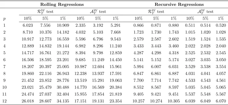
Our proposed procedure specialized to tests of forecast optimality is the following. Let RWT = sup R2fR;:::Rg [LbT(R)0bR1LbT (R)]; (14) and AWT = 1 R R+ 1 R X R=R [LbT(R)0bR1LbT (R)]; (15) where LbT (R) P 1=2 PT
t=RLbt+h;and bR is a consistent estimator of . Reject the null
hypothesisH0 : limT!1E(Lt+h( )) = 0for allRat the signi…cance level whenRWT > kR
for the sup-type test and when AW
T > kA;p;W for the average-type test, where the critical
valueskR;p;W and kA;p;W for = 0:15are reported in Table 3.
A simple, consistent estimator for can be obtained by following West and McCracken (1998). West and McCracken (1998) have shown that it is very important to allow for a general variance estimator that takes into account estimation uncertainty and/or correcting the statistics by the necessary adjustments. See West and McCracken’s (1998) Table 2 for details on the necessary adjustment procedures for correcting for parameter estimation uncertainty. The same procedures should be implemented to obtain correct inference in regression-based tests in our setup. For convenience, we discuss in detail how to construct a consistent variance estimate in the leading case of Mincer and Zarnowitz’s (1969) regressions in Appendix B in Inoue and Rossi (2012) in either rolling, recursive or …xed estimation schemes.
Historically, researchers have estimated the alternative regression: bvt+h =bgt0 b(R)+bt+h,
where b(R) = P 1PT t=Rbgtbg0t
1
P 1PT
t=Rbgtbvt+h and bt+h is the …tted error of the
regression, and tested whether the coe¢ cients equal zero. It is clear that under the additional assumption that E(gtg0t) is full rank (a maintained assumption in that literature) the two
procedures share the same null hypothesis and are therefore equivalent. However, in this case it is convenient to de…ne the following re-scaled Wald test:
WT(r)(R) = b(R)0 Vb 1(R)
b(R);
where Vb (R) is a consistent estimate of the asymptotic variance of b(R); V : We propose the following tests:
RWT = sup R2fR;:::Rg b(R)0 Vb 1(R)b(R); (16) and AWT = 1 R R+ 1 R X R=R b(R)0 Vb 1(R)b(R): (17)
Reject the null hypothesis H0 : limT!1E[b(R)] = 0 for all R when RT > kR;p;W for the
sup-type test and when AT > kA;W
;p for the average-type test. Simulated values ofkR;p;W and
kA;W
;p for = 0:15 and various values ofp are reported in Table 3.
Under more general speci…cations for the loss function, the properties of forecast errors previously discussed may not hold. In those situations, Patton and Timmermann (2007) show that a “generalized forecast error” does satisfy the same properties. The procedures that we propose can also be applied to Patton and Timmermann’s (2007) generalized forecast error.
3
Robust Tests of Predictive Accuracy When the
Win-dow Size is Small
All the tests considered so far rely on the assumption that the window is a …xed fraction of the total sample size, asymptotically. This assumption rules out the tests by Clark and West (2006, 2007) and Giacomini and White (2005), which rely on a constant (…xed) window size. Propositions 2 and 3 extend our methodology in these two cases by allowing the window size to be …xed.
First, we will consider a version of Clark and West’s (2006, 2007) test statistics. Monte Carlo evidence in Clark and West (2006, 2007) and Clark and McCracken (2001, 2005) shows that Clark and West’s (2007) test has power broadly comparable to the power of an F-type test of equal MSE. Clark and West’s (2006, 2007) test is also popular because it has the advantage of being approximately normal, which permits the tabulation of asymptotic critical values applicable under multi-step forecasting and conditional heteroskedasticity. Before we get into details, a word of caution: our setup requires strict exogeneity of the regressors, which is a very strong assumption in time series application. When the window size diverges to in…nity, the correlation between the rolling regression estimator and the regressor vanishes even when the regressor is not strictly exogenous. When the window size is …xed relative to the sample size, however, the correlation does not vanish even asymptotically when the regressor is not strictly exogenous. When the null model is the no-change forecast model as required by the original test of Clark and West (2006, 2007) when the window size is …xed, the assumption of strict exogeneity can be dropped and our test statistic becomes identical to theirs.
Consider the following nested forecasting models: yt+h = 01x1t+e1;t+h; (18) yt+h = 02x2t+e2;t+h; (19) where x2;t = [x01;t zt0]0. Let ^1t(R) = ( Pt s=t R+1x1;sx01;s) 1 Pt s=t R+1x1;sys+h and ^ 2t(R) = ( Pt s=t R+1x2;sx02;s) 1 Pt
s=t R+1x2;sys+h and let ^e1;t+h(R)and ^e2;t+h(R)denote the corresponding models’h-steps-ahead forecast errors. Note that, since the models are nested, Clark and West’s (2007) test is one sided. Under the null hypothesis that 2 = [ 10 00]0, the
M SP E-adjusted of Clark and West (2007) can be written as:
M SP E-adjusted = P 1 T X t=R ^ e21;t+h(R) ^e22;t+h(R) (^y1;t+h y^2;t+h)2 = 2P 1 T X t=R ^ e1;t+h(R) [^e1;t+h(R) e^2;t+h(R)] where P 1PT
t=R(^y1;t+h y^2;t+h)2 is the adjustment term. When R is …xed, as Clark and
West (2007, p.299) point out, the mean ofM SP E-adjustedis nonzero unlessx1tis null. We
consider an alternative adjustment term so that the adjusted loss di¤erence will have zero mean. Suppose that 2 = [ 10 00]0 and that x
2;t is strictly exogenous. Then we have
E[(^e21;t+h e^2;t+h)2] = E[(yt+h y^1;t+h)2] E[(yt+h y^2;t+h)2] = E(yt2+h 2yt+hx01t^1t+ ^y 2 1;t+h) E(y 2 t+h 2yt+hx02t^2t+ ^y 2 2;t+h) = E[^y12;t+h y^22;t+h] + 2E[yt+h(x02t^2t x01t^1t)] = E[^y12;t+h y^22;t+h] + 2Efyt+h[x02t(^2t 2) x01t(^1t 1)]g (20) = E[^y12;t+h y^22;t+h] + 2E[ 10x1t(x02t(^2t 2) x01t(^1t 1))](21) = E[^y12;t+h y^22;t+h];
where the fourth equality follows from the null hypothesis, 2 = [ 10 00]0, the …fth equality follows from the null that e2;t+h is orthogonal to the information set at time t and the last
equality from the strict exogeneity assumption. Thus t+h(R) e^21;t+h(R) ^e22;t+h(R)
[^y12;t+h(R) y^22;t+h(R)] has zero mean even whenx1t is not null provided that the regressors
are strictly exogenous.
When R is …xed, Clark and West’s adjustment term is valid if the null model is the no-change forecast model, i.e., x1t is null. When x1t is null, the second term on the right-hand
side of equation (20) is zero even when x2t is not strictly exogenous, and our adjustment
Proposition 2 (Out-of-Sample Robust Test with Fixed Window Size I. ) Suppose
that: (a) either x1t is null or E(e2tjx2s) = 0 for all s and t such that t R s t+R; (b)
f[e1;t+1; x01;t+1; zt0+1]0g is -mixing of size r=(r 2); (c) [e1;t+h; x01;t; z0t; ^1;t(R)0;^1;t(R+ 1)0;
:::;^1;t(R); ^2;t(R)0;^
2;t(R+ 1)0; :::; ^2;t(R)]0 has …nite4r-th moments uniformly int; (d) R
and R are …xed constants. Then
R 2 6 6 6 6 6 4 P 1=2PT t=R t+h(R) P 1=2PTt=R+1 t+h(R+ 1) .. . P 1=2PT t=R t+h(R) 3 7 7 7 7 7 5 d ! N(0; )
where is the long-run covariance matrix, =P1j= 1 j and
j = E 8 > > > > > < > > > > > : 2 6 6 6 6 6 4 t+h(R) t+h(R+ 1) .. . t+h(R) 3 7 7 7 7 7 5 2 6 6 6 6 6 4 t+h j(R) t+h j(R+ 1) .. . t+h j(R) 3 7 7 7 7 7 5 09 > > > > > = > > > > > ; :
Let r =R R+ 1: The test that we propose is:
CWT 0Rb 1
R d
! 2r; (22)
where b is a consistent estimate of . The null hypothesis is rejected at the signi…cance
level for any R when CWT > 2r; , where 2r; is the (1 )-th quantile of a chi-square
distribution with r degrees of freedom.
The proof of this proposition follows directly from Corollary 24.7 of Davidson (1994, p.387). Assumption (a) is necessary for t+h(R)to have zero mean and is satis…ed under the
assumption discussed by Clark and West (x1t is not null) or under the assumption that x2t
is strictly exogenous. The latter assumption is very strong in the applications of interest. We also consider the Giacomini and White’s (2005) framework. Proposition 3 provides a methodology that can be used to robustify their test for unconditional predictive ability with respect to the choice of the window size.
Proposition 3 (Out-of-sample Robust Tests with Fixed Window Size II. ) Suppose the assumptions of Theorem 4 in Giacomini and White (2005) hold, and that there exists a
unique window sizeR2 fR; :::; Rgfor which the null hypothesisH0 : limT!1E h LT bt;R;bt;R i = 0 holds. Let GWT = inf R2fR;:::;Rgj LT (R)j; (23) where LT (R) b1 RT 1=2PT
t=R LT(bt;R;bt;R); R and R are …xed constants, and ^
2 R is a
consistent estimator of 2. Under the null hypothesis,
GWT d
!N(0;1);
The null hypothesis for the GWT test is rejected at the signi…cance level in favor of the
two-sided alternative limT!1E
h
LT bt;R;bt;R
i
6
= 0 for any R when GWT > z =2; where
z =2 is the 100 (1 =2) % quantile of a standard normal distribution.
Note that, unlike the previous cases, in this case we consider theinf( )over the sequence of out-of-sample tests rather than the sup( ). The reason why we do so is related to the special nature of Giacomini and White’s (2005) null hypothesis: if their null hypothesis is true for one window size then it is necessarily false for other window sizes; thus, the test statistic is asymptotically normal for the former, but diverges for the others. That is why it makes sense to take theinf( ). Our assumption that the null hypothesis holds only for one value of R may sound peculiar, but the unconditional predictive ability test of Giacomini and White (2005) typically implies a unique value of R, although there is no guarantee that the null hypothesis of Giacomini and White (2006) holds in general. For example, consider the the case where data are generated from yt = 2 +et where et
iid
(0; 2), and let the researcher be interested in comparing the MSFE of a model where yt is unpredictable
(yt =e1t) with that of a model whereyt is constant (yt= 2+e2;t). Under the unconditional
version of the null hypothesis we have E[yt2+1 (yt+1 R 1 tj=t R+1yj)2] = 0, which in
turn implies 22
2
R = 0. Thus, if the null hypothesis holds then it holds with a unique
value of R. Our proposed test protects applied researchers from incorrectly rejecting the null hypothesis by choosing an ad hoc window size, which is important especially for the Giacomini and White’s (2005) test, given its sensitivity to data snooping over window sizes. The proof of Proposition 3 is provided in Appendix A in Inoue and Rossi (2012). Note that one might also be interested in a one-sided test, whereH0 : limT!1E
h
LT bt;R;bt;R
i
= 0 versus the alternative that limT!1E
h
LT bt;R;bt;R
i
> 0. In that case, construct
GWT = infR=R;:::R LT (R); and reject when GWT > z ; where z =2 is the 100(1 ) % quantile of a standard normal distribution.
4
Monte Carlo evidence
In this section, we evaluate the small sample properties of the methods that we propose and compare them with the methods existing in the literature. We consider both nested and non-nested models’ forecast comparisons, as well as forecast rationality. For each of these tests under the null hypothesis, we allow for three choices of , one-step-ahead and multi-step-ahead forecasts, and multiple regressors of alternative models to see if and how the size of the proposed tests is a¤ected in small samples. We consider the no-break alternative hypothesis and the one-time-break alternative to compare the power of our proposed tests with that of the conventional tests. Below we report rejection frequencies at the 5% nominal signi…cance level to save space.
For the nested models comparison, we consider a modi…cation of the DGP (labeled “DGP 1”) that follows Clark and McCracken (2005a) and Pesaran and Timmermann (2007). Let
0 B B @ yt+1 xt+1 zt+1 1 C C A= 0 B B @ 0:3 dt;T 01 (k2 1) 0 0:5 01 (k2 1) 0 0(k2 1) 1 0:5 Ik2 1 1 C C A 0 B B @ yt xt zt 1 C C A+ 0 B B @ uy;t+1 ux;t+1 uz;t+1 1 C C A; t= 1; :::; T 1; where y0 = x0 = 0, z0 = 0(k2 1) 1, [uy;t+1 ux;t+1 u0z;t+1]0 iid N(0(k2+1) 1; Ik2+1) and Ik2+1
denotes an identity matrix of dimension(k2+ 1) (k2+ 1). We compare the following two nested models’forecasts foryt+h:
Model 1 forecast : b1;tyt (24)
Model 2 forecast : b1;tyt+b02;txt+b03;tzt;
and both models’ parameters are estimated by OLS in rolling windows of size R: Under the null hypothesis dt;T = 0 for all t and we consider h = 1;4;8, k2 = 1;3;5 and T = 50;100;200;500. We consider several horizons (h) to evaluate how our tests perform at both the short and long horizons that are typically considered in the literature. We consider several extra-regressors (k2) to evaluate how our tests perform as the estimation uncertainty induced by extra regressors increases. Finally, we consider several sample sizes (T) to evaluate how our tests perform in small samples. Under the no-break alternative hypothesis dt;T = 0:1 or
dt;T = 0:2 (h = 1, k2 = 1 and T = 200). Under the one-time-break alternative hypothesis,
dt;T = 0:5 I(t ) for 2 f40;80;120;160g, (h= 1, k2 = 1 and T = 200).
“DGP2”): 0 B B @ yt+1 xt+1 zt+1 1 C C A= 0 B B @ 0:3 dt;T 0:5 01 (k 2) 0 0:5 0 01 (k 2) 0(k 1) 1 0(k 1) 1 0:5I(k 1) 1 C C A 0 B B @ yt xt zt 1 C C A+ 0 B B @ uy;t+1 ux;t+1 uz;t+1 1 C C A; t= 1; :::; T 1;
where y0 =x0 = 0, z0 = 0(k 1) 1, and[uy;t+1 ux;t+1 u0z;t+1]0 iid
N(0(k+1) 1; Ik+1). We compare the following two non-nested models’forecasts for yt+h:
Model 1 forecast : b1yt+b2xt (25)
Model 2 forecast : b1yt+b02zt;
and both models’parameters are estimated by OLS in rolling windows of sizeR. Under the null hypothesis dt;T = 0:5 for all t: Again, we consider several horizons, number of
extra-regressors and sample sizes: h = 1;4;8, k = 2;4;6 and T = 50;100;200;500. We use the two-sided version of our test. Note that, for non-nested models with k > 2, one might expect that, in …nite samples, model 1 would be more accurate than model 2 because model 2 includes extraneous variables, however. Under the no-break alternative hypothesisdt;T = 1
ordt;T = 1:5(h= 1,k = 2 and T = 200). Under the one-time-break alternative hypothesis,
dt;T = 0:5 I(t ) + 0:5 for 2 f40;80;120;160g, (h= 1,k = 2 and T = 200).
“DGP3” is designed for regression-based tests and is a modi…cation of the Monte Carlo design in West and McCracken (1998). Let
yt+1 = t;T Ip+ 0:5yt+"t+1; t= 1; :::; T;
where yt+1 is a p 1 vector and "t+1 iid
N(0p 1; Ip). We generate a vector of variables
rather than a scalar because in this design we are interested in testing whether the forecast error is not only unbiased but also uncorrelated with information available up to time t, including lags of the additional variables in the model. Let y1;t be the …rst variable in the
vector yt. We estimate y1;t+h = 0yt+vt+h by rolling regressions and test E(vt+h) = 0
and E(ytvt+h) = 0 for h = 1;4;8 and p = 1;3;6. We let t;T = 0:5 or t;T = 1 under the
no-break alternative and t;T = 0:5 I(t ) for 2 f40;80;120;160g under the one-time
break alternative (h= 1, p= 1 and T = 200).
For the forecast comparison tests with a …xed window size, we consider the following DGP (labeled “DGP4”): yt+1 = Rxt +"t+1; t = 1; :::; T;where xt and "t+1 are i.i.d. standard Normal independent of each other. We compare the following two nested models’
forecasts for yt: a …rst model is a no-change forecast model, e.g. the random walk
fore-cast for a target variable de…ned in …rst di¤erences, and the second is a model with the regressor; that is, Model 1 forecast equals zero and Model 2 forecast equals bt;Rxt;where
bt;R = t P j=t R+1 x2 t ! 1 t P j=t R+1
xtyt. To ensure that the null hypothesis in Proposition 3
holds for one of the window sizes, R, we let R = (R 2) 1=2
. The number of Monte Carlo replications is 5,000. To ensure that the null hypothesis in Proposition 2 holds, we let
R = = 0.
The size properties of our test procedures in small samples are …rst evaluated in a series of Monte Carlo experiments. We report empirical rejection probabilities of the tests we propose at the 5% nominal level. In all experiments except DGP4, we investigate sample sizes whereT = 50;100;200 and500 and set = 0:05;0:15;0:25and = 1 . For DGP4, we let P = 100; 200 and 500 and let R = 20 or 30 and R = R+ 5: Note that in design 4 we only consider …ve values of R since the window size is small by assumption, and that limits the range of values we can consider. Tables 4, 5 and 6 report results for the R"
T and
A"
T tests for the nested models comparison (DGP1), the RT and AT tests for non-nested
models comparison (DGP2), and RW
T and AWT for the regression-based tests of predictive
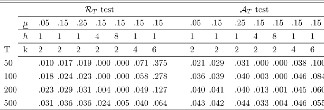
ability (DGP3), respectively. For the multiple horizon case, in nested and regression-based inference we use the heteroskedasticity and autocorrelation consistent (HAC) estimator with the truncated kernel, bandwidth h 1and the adjustment proposed by Harvey, Leybourne and Newbold (1997), as suggested by Clark and McCracken (2011a, Section 4), and then bootstrap the test statistics using the parametric bootstrap based on the estimated VAR model as suggested by Clark and McCracken (2005). Note that designs that have the same parameterization do not have exactly the same rejection frequencies since the Monte Carlo experiments are ran independently for the various cases we study, and therefore there are small di¤erences due to simulation noise. The number of Monte Carlo simulations is set to 5,000 except that it is set to 500 and the number of bootstrap replications is 199 in Tables 4 and 6 whenh >1.
Table 4 shows that the nested model comparison tests (i.e., RE
T and AET tests) have good
size properties overall. Except for small sample sizes, they perform well even in the multiple forecast horizon and multiple regressor cases. Although the e¤ect of the choice of becomes smaller as the sample size grows, the RE
T test tends to over-reject with smaller values of .
TheAE
T test is less sensitive to the choice of . The tests implemented with = 0:05tend to
recommend that = 0:15. Table 5 shows that the non-nested model comparison tests (RT
and AT tests) also have good size properties although they tend to be slightly under-sized.
They tend to be more under-sized as the forecast horizon grows, thus suggesting that the test is less reliable for horizons greater than one period. The RT test tends to reject too often
when there are many regressors (p= 6). Note that, by showing that the test is signi…cantly oversized in small samples, the simulation results con…rm that for non-nested models with
p > 1model 1 should be more accurate than model 2 in …nite samples, as expected. Table 6 shows the size properties of the regression-based tests of predictive ability (RW
T and AWT
tests). The tests tend to reject more often as the the forecast horizon increases and less often as the number of restrictions increases.
Table 7 reports empirical rejection frequencies for DGP4. The left panel shows results for the GWT test, eq. (23), reported in the column labeled “GWT test”. The table shows
that our test is conservative when the number of out-of-sample forecasts P is small, but otherwise it is controlled. Similar results hold for the CWT test discussed in Proposition 2.
Next, we consider three additional important issues. First, we evaluate the power prop-erties of our proposed procedure in the presence of departures from the null hypothesis in small samples. Second, we show that traditional methods, which rely on an “ad-hoc”window size choice, may have no power at all to detect predictive ability. Third, we demonstrate traditional methods are subject to data mining (i.e. size distortions) if they are applied to many window sizes without correcting the appropriate critical values.
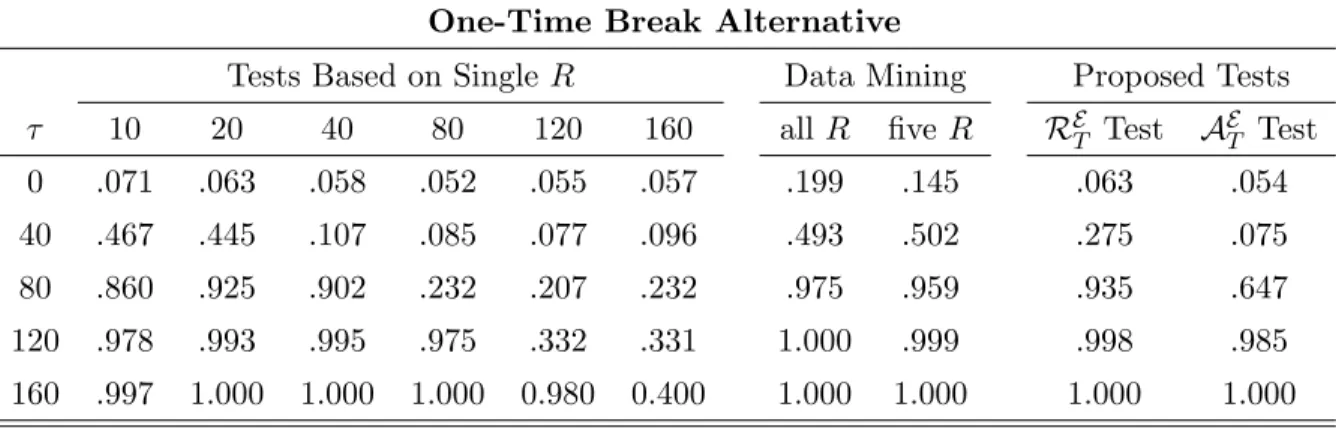
Tables 8, 9 and 10 report empirical rejection rates for the Clark and McCracken’s (2001) test under DGP1 withh= 1andp= 0, the non-nested model comparison test of Diebold and Mariano (1995), West (1996) and McCracken (2000) under DGP2 withh= 1andp= 1, and West and McCracken’s (1998) regression-based test of predictive ability under DGP3 with
h = 1 and p = 1, respectively. In each table, the columns labeled “Tests Based on Single
R” report empirical rejection rates implemented with a speci…c value of R which would correspond to the case of a researcher who has chosen one “ad-hoc”window sizeR, has not experimented with other choices, and thus might have missed predictive ability associated with alternative values ofR. The columns labeled “Data Mining”report empirical rejection rates incurred by a researcher who is searching across all values ofR2 f30;31; :::;170g(“all
R”) and across …ve values,R2 f20;40;80;120;160g. That is, the researcher reports results associated with the most signi…cant window size without taking into account the search procedure when doing inference. The critical values used for these conventional testing procedures are based on Clark and McCracken (2001) and West and McCracken (1998)
for Tables 8 and 10 and are equal to 1.96 for Table 9. Note that to obtain critical values for the ENCNEW test and regression-based test of predictive ability that are not covered by their tables, the critical values are estimated from 50,000 Monte Carlo simulations in which the Brownian motion is approximated by normalized partial sums of 10,000 standard normal random variates. For the non-nested model comparison test, parameter estimation uncertainty is asymptotically irrelevant by construction and the standard normal critical values can be used. The nominal level is set to 5%, = 0:15, = 0:85;and the sample size is 200.
The …rst row of each panel reports the size of these testing procedures and shows that all tests have approximately the correct size except the data mining procedure, which has size distortions and leads to too many rejections with probabilities ranging from 0.175 to 0.253. Even when only …ve window sizes are considered, data mining leads to falsely rejecting the null hypothesis with probability more than 0.13. This implies that the empirical evidence in favor of the superior predictive ability of a model can be spurious if evaluated with the incorrect critical values. Results in Inoue and Rossi (2012, Panel A in Tables 8, 9 and 10) show that the conventional tests and proposed tests have power against the standard no-break alternative hypothesis. Unreported results show that while the power of the RE
T test
is increasing in , it is decreasing in for the RT and RWT tests. The power of theAET,AT
and AW
T tests is not sensitive to the choice of .
The tables demonstrate that, in the presence of a structural break the tests based on an “ad-hoc” rolling window size can have low power depending on the window size and the break location. The evidence highlights the sharp sensitivity of power of all the tests to the timing of the break relative to the forecast evaluation window, and shows that, in the presence of instabilities, our proposed tests tend to be more powerful than some of the tests based on an ad-hoc window size, whose power properties crucially depend on the window size. Against the break alternative, the power of the proposed tests tend to be decreasing in . Based on these size and power results we recommend = 0:15 in Section 2, which provides a good performance overall.
Finally, we show that the e¤ects of data mining are not just a small sample phenomenon. We quantify the e¤ects of data mining asymptotically by using the limiting distributions of existing test statistics. We design a Monte Carlo simulation where we generate a large sample of data (T=2000) and use it to construct limiting approximations to the test statistics described in Appendix B in Inoue and Rossi (2012). For example, in the non-nested models comparison case withp= 1, the limiting distribution of the Diebold and Mariano (1995) test
statistic for a given = lim
T!1
R
T is(1 ) 1=2
jB(1) B( )j; the latter can be approximated in large samples by 1 RT 1=2jP 1=2 PT
t=R tj
, where t iidN(0;1). We simulate the latter for many window sizes R and then calculate how many times, on average across 50,000 Monte Carlo replications, the resulting vector of statistics exceed the standard normal critical values for a 5% nominal size. Table 11 reports the results, which demonstrate that the over-rejections of traditional tests when researchers data snoop over window sizes persist asymptotically.
5
Empirical evidence
The poor forecasting ability of economic models of exchange rate determination has been recognized since the works by Meese and Rogo¤ (1983a,b), who established that a random walk forecasts exchange rates better than any economic models in the short run. Meese and Rogo¤’s (1983a,b) …nding has been con…rmed by several researchers and the random walk is now the yardstick of comparison for the evaluation of exchange rate models. Recently, Engel, Mark and West (2007) and Molodtsova and Papell (2009) documented empirical evidence in favor of the out-of-sample predictability of some economic models, especially those based on the Taylor rule. However, the out-of-sample predictability that they report depends on certain parameters, among which the choice of the in-sample and out-of-sample periods and the size of the rolling window used for estimation. The choice of such parameters may a¤ect the outcome of out-of-sample tests of forecasting ability in the presence of structural breaks. Rossi (2006) found empirical evidence of instabilities in models of exchange rate determination; Giacomini and Rossi (2010) evaluated the consequences of instabilities in the forecasting performance of the models over time; Rogo¤ and Stavrakeva (2008) also question the robustness of these results to the choice of the starting out-of-sample period. In this section, we test the robustness of these results to the choice of the rolling window size. It is important to notice that it is not clear a-priori whether our test would …nd more or less empirical evidence in favor of predictive ability. In fact, there are two opposite forces at play. By considering a wide variety of window sizes, our tests might be more likely to …nd empirical evidence in favor of predictive ability, as our Monte Carlo results have shown. However, by correcting statistical inference to take into account the search process across multiple window sizes, our tests might at the same time be less likely to …nd empirical evidence in favor of predictive ability.
Let st denote the logarithm of the bilateral nominal exchange rate, where the exchange
rate is de…ned as the domestic price of foreign currency. The rate of growth of the exchange rate depends on its deviation from the current level of a macroeconomic fundamental. Let
ft denote the long-run equilibrium level of the nominal exchange rate as determined by the
macroeconomic fundamental, and zt=ft st. Then,
st+1 st= + zt+"t+1 (26)
where "t+1 is an unforecastable error term.The …rst model we consider is the Uncovered Interest Rate Parity (UIRP). In the UIRP model,
ftU IRP = (it it) +st; (27)
where(it it)is the short-term interest di¤erential between the home and the foreign
coun-tries.
The second model we consider is a model with Taylor rule fundamentals, as in Molodtsova and Papell (2009) and Engel, Mark and West (2007). Let tdenote the in‡ation rate in the
home country, t denote the in‡ation rate in the foreign country, denote the target level of in‡ation in each country, ytgap denote the output gap in the home country andytgap denote the output gap in the foreign country. Note that the output gap is the percentage di¤erence between actual and potential output at time t, where the potential output is the linear time trend in output, and that Taylor rule speci…cation is one for which Papell and Molodtsova (2009) …nd the least empirical evidence of predictability so our results can be interpreted as a lower bound on the predictability of Taylor rules that they consider. Since the di¤erence in the Taylor rule of the home and foreign countries impliesit it = ( t t)+ (y
gap
t y
gap t ),
we have that the latter determines the long run equilibrium level of the nominal exchange rate: ftT AY LOR = ( t t) + (y gap t y gap t ) +st: (28)
The benchmark model, against which the forecasts of both models (27) and (28) are evaluated, is the random walk, according to which the exchange rate changes are forecast to be zero. We chose the random walk without drift to be the benchmark model because it is the toughest benchmark to beat (see Meese and Rogo¤, 1983a,b). We use monthly data from the International Financial Statistics database (IMF) and from the Federal Reserve Bank of St. Louis from 1973:3 to 2008:1 for Japan, Switzerland, Canada, Great Britain, Sweden, Germany, France, Italy, the Netherlands, and Portugal. Data on interest rates were incomplete for Portugal and the Netherlands, so we do not report UIRP results for these
countries. The former database provides the seasonally adjusted industrial production index for output, and the 12-month di¤erence of the CPI for the annual in‡ation rate, and the interest rates. The latter provides the exchange rate series. The two models’rolling forecasts (based on rolling windows calculated over an out-of-sample portion of the data starting in 1983:2) are compared to the forecasts of the random walk, as in Meese and Rogo¤ (1983a,b). We focus on the methodologies in Section 2.2 since the models are nested. In our exercise, = 0:15, which implies R = T and R= (1 )T; the total sample size T depends on the country, and the values ofR and R are shown on the x-axes in Figures 1 and 2, and o¤er a relatively large range of window sizes, all of which are su¢ ciently large for asymptotic theory to provide a good approximation.
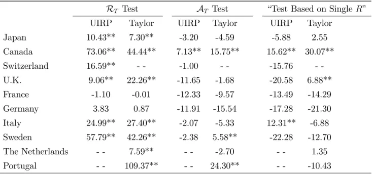
Empirical results for selected countries are shown in Table 12 and Figure 1 (see Inoue and Rossi, 2012, for detailed results on other countries/models). The column labeled “Test Based on Single R” in Table 12 reports the empirical results in the literature based on a window sizeRequal to 120, the same window size used in Molodtsova and Papell (2009). According to the “Test Based on SingleR;”the Taylor model signi…cantly outperforms a random walk for Canada and the U.K. at 5% signi…cance level, whereas the UIRP model outperforms the random walk for Canada and Italy at the 5% signi…cance level. According to our tests, instead, the empirical evidence in favor of predictive ability is much more favorable. Figure 1 reports the estimated Clark and McCracken’s (2001) test statistic for the window sizes we consider for the UIRP model. Note that the R"
T test rejects if, for any window size R
(reported on the x-axis), the test statistic is above the critical value line (dotted lines). In particular, the predictive ability of the economic models tends to show up at smaller window sizes, as the …gures show. This suggests that the empirical evidence in favor of predictive ability may be driven by the existence of instabilities in the predictive ability, for which rolling windows of small size are advantageous. One should also be aware of the possibility of data snooping over country-model pairs; we refer to Molodtsova and Papell (2009).
6
Conclusions
This paper proposes new methodologies for evaluating economic models’forecasting perfor-mance that are robust to the choice of the estimation window size. These methodologies are noteworthy since they allow researchers to reach empirical conclusions that do not depend on a speci…c estimation window size. We show that tests traditionally used by forecasters su¤er from size distortions if researchers report, in reality, the best empirical result over various
window sizes, but without taking into account the search procedure when doing inference in practice. Traditional tests may also lack power to detect predictive ability when imple-mented for an "ad-hoc" choice of the window size. Finally, our empirical results demonstrate that the recent empirical evidence in favor of exchange rate predictability is even stronger when allowing a wider search over window sizes.
References
[1] Andrews, D.W.K. (1993), “Tests of Parameter Instability and Structural Change With Unknown Change Point,”Econometrica, 61, 821–856.
[2] Billingsley, P. (1968), Convergence of Probability Measures, John Wiley & Sons: New York, NY.
[3] Chao, J.C., V. Corradi and N.R. Swanson (2001), “An Out-of-Sample Test for Granger Causality,”Macroeconomic Dynamics.
[4] Cheung, Y., M.D. Chinn and A.G. Pascual (2005), “Empirical Exchange Rate Models of the Nineties: Are Any Fit to Survive?,”Journal of International Money and Finance
24, 1150-1175.
[5] Chinn, M. (1991), “Some Linear and Nonlinear Thoughts on Exchange Rates,”Journal
of International Money and Finance 10, 214-230.
[6] Chong, Y.Y. and D.F. Hendry (1986), “Econometric Evaluation of Linear Macroeco-nomic Models,”Review of Economic Studies 53, 671-690.
[7] Clark, T.E. and M.W. McCracken (2001), “Tests of Equal Forecast Accuracy and En-compassing for Nested Models,”Journal of Econometrics 105(1), 85-110.
[8] Clark, T.E. and M.W. McCracken (2005a), “The Power of Tests of Predictive Ability in the Presence of Structural Breaks,”Journal of Econometrics 124, 1-31.
[9] Clark, T.E. and M.W. McCracken (2005b), “Evaluating Direct Multistep Forecasts,”
Econometric Reviews 24(3), 369-404.
[10] Clark, T.E. and M.W. McCracken (2009), “Improving Forecast Accuracy by Combining Recursive and Rolling Forecasts,”International Economic Review, 50(2), 363-395.
[11] Clark, T.E. and M.W. McCracken (2010), “Reality Checks and Nested Forecast Model Comparisons,”mimeo, St. Louis Fed.
[12] Clark, T.E. and M.W. McCracken (2011a), “Advances in Forecast Evaluation,” in: G. Elliott and A. Timmermann (eds.),Handbook of Economic Forecasting, Vol. 2, Elsevier, forthcoming.
[13] Clark, T.E. and M.W. McCracken (2011b), “Tests of Equal Forecast Accuracy for Over-lapping Models,”Federal Reserve Bank of St. Louis Working Paper 2011-024,.
[14] Clark, T.E. and K.D. West (2006), “Using Out-of-Sample Mean Squared Prediction Errors to Test the Martingale Di¤erence Hypothesis,”Journal of Econometrics 135, 155–186.
[15] Clark, T.E. and K.D. West (2007), “Approximately Normal Tests for Equal Predictive Accuracy in Nested Models,”Journal of Econometrics 138, 291-311.
[16] Clements, M.P. and D.F. Hendry (1993), “On the Limitations of Comparing Mean Square Forecast Errors,”Journal of Forecasting 12, 617-637.
[17] Davidson, J. (1994), Stochastic Limit Theory: An Introduction for Econometricians. Oxford: Oxford University Press.
[18] Diebold, F.X. and J. Lopez (1996), “Forecast Evaluation and Combination,” in
Hand-book of Statistics, G.S. Maddala and C.R. Rao eds., North-Holland, 241–268.
[19] Diebold, F.X. and R.S. Mariano (1995), “Comparing Predictive Accuracy,”Journal of
Business and Economic Statistics, 13, 253-263.
[20] Engel, C., N. Mark and K.D. West, “Exchange Rate Models Are Not as Bad as You Think,” in: NBER Macroeconomics Annual, Daron Acemoglu, Kenneth S. Rogo¤ and Michael Woodford, eds. (Cambridge, MA: MIT Press, 2007).
[21] Giacomini, R. and B. Rossi (2010), “Model Comparisons in Unstable Environments”,
Journal of Applied Econometrics 25(4),595-620.
[22] Giacomini, R. and H. White (2006), “Tests of Conditional Predictive Ability,”
[23] Gourinchas, P.O., and H. Rey (2007), “International Financial Adjustment,”The
Jour-nal of Political Economy 115(4), 665-703.
[24] Granger, C.W.J. and P. Newbold (1986), Forecasting Economic Time Series (2nd ed.), New York: Academic Press.
[25] Hansen, B.E. (1992), “Convergence to Stochastic Integrals for Dependent Heterogeneous Processes,”Econometric Theory 8, 489-500.
[26] Hansen, P.R. and A. Timmermann (2011), “Choice of Sample Split in Out-of-Sample Forecast Evaluation”, mimeo.
[27] Harvey, D.I., S.J. Leybourne and P. Newbold (1997), “Testing the Equality of Prediction Mean Squared Errors,”International Journal of Forecasting, 13, 281–291.
[28] Harvey, D.I., S.J. Leybourne and P. Newbold (1998), “Tests for Forecast Encompass-ing,”Journal of Business and Economic Statistics 16 (2), 254-259.
[29] Inoue, A. and B. Rossi (2011), “Out-of-Sample Forecast Tests Robust to the Choice of Window Size”, ERID Working Paper, Duke University.
[30] Inoue, A. and B. Rossi (2012), “Out-of-Sample Forecast Tests Robust to the Choice of Window Size”, JBES website.
[31] McCracken, M.W. (2000), “Robust Out-of-Sample Inference,”Journal of Econometrics
99, 195-223.
[32] Meese, R. and K.S. Rogo¤ (1983a), “Exchange Rate Models of the Seventies. Do They Fit Out of Sample?,”The Journal of International Economics 14, 3-24.
[33] Meese, R. and K.S. Rogo¤ (1983b), “The Out of Sample Failure of Empirical Exchange Rate Models,” in Jacob Frankel (ed.), Exchange Rates and International
Macroeco-nomics, Chicago: University of Chicago Press for NBER.
[34] Mincer, J. and V. Zarnowitz (1969), “The Evaluation of Economic Forecasts,” in
Eco-nomic Forecasts and Expectations, ed. J. Mincer, New York: National Bureau of
Eco-nomic Research, 81–111.
[35] Molodtsova, T. and D.H. Papell (2009), “Out-of-Sample Exchange Rate Predictability with Taylor Rule Fundamentals,”Journal of International Economics 77(2).
[36] Newey, W. and K.D. West (1987), “A Simple, Positive Semi-De…nite, Heteroskedasticity and Autocorrelation Consistent Covariance Matrix,”Econometrica 55, 703-708.
[37] Patton, A.J. and A. Timmermann (2007), “Properties of Optimal Forecasts Under Asymmetric Loss and Nonlinearity,”Journal of Econometrics 140, 884-918.
[38] Paye, B. and A. Timmermann (2006), “Instability of Return Prediction Models,”
Jour-nal of Empirical Finance 13(3), 274-315.
[39] Pesaran, M.H., D. Pettenuzzo and A. Timmermann (2006), “Forecasting Time Series Subject to Multiple Structural Breaks,”Review of Economic Studies 73, 1057-1084. [40] Pesaran, M.H. and A. Timmermann (2005), “Real-Time Econometrics,”Econometric
Theory 21(1), pages 212-231.
[41] Pesaran, M.H. and A. Timmermann (2007), “Selection of Estimation Window in the Presence of Breaks,”Journal of Econometrics 137(1), 134-161.
[42] Qi, M. and Y. Wu (2003), “Nonlinear Prediction of Exchange Rates with Monetary Fundamentals,”Journal of Empirical Finance 10, 623-640.
[43] Rogo¤, K.S. and V. Stavrakeva, “The Continuing Puzzle of Short Horizon Exchange Rate Forecasting,”NBER Working paper No. 14071, 2008.
[44] Rossi, B. (2006), “Are Exchange Rates Really Random Walks? Some Evidence Robust to Parameter Instability,”Macroeconomic Dynamics 10(1), 20-38.
[45] Rossi, B., and T. Sekhposyan (2010), “Understanding Models’ Forecasting Perfor-mance,”mimeo, Duke University.
[46] Rossi, B., and A. Inoue (2011), “Out-of-Sample Forecast Tests Robust to the Choice of Window Size,” mimeo, Duke University and North Carolina State University.
[47] Stock, J.H. and M.W. Watson (2003a), “Forecasting Output and In‡ation: The Role of Asset Prices,”Journal of Economic Literature.
[48] West, K.D. (1996), “Asymptotic Inference about Predictive Ability,”Econometrica, 64, 1067-1084.
[49] West, K.D., and M.W. McCracken (1998), “Regression-Based Tests of Predictive Abil-ity,”International Economic Review,39, 817–840.
Tables and Figures
Table 1. Critical Values for Non-Nested Model Comparisons
Panel A. Two-Sided Critical Values Panel B. One-Sided Critical Values
RT test AT test RT test AT test
10% 5% 1% 10% 5% 1% 10% 5% 1% 10% 5% 1% 0.15 2.465 2.754 3.337 1.462 1.739 2.292 2.127 2.458 3.106 1.134 1.454 2.073 0.20 2.398 2.697 3.282 1.489 1.771 2.345 2.057 2.399 3.059 1.158 1.488 2.116 0.25 2.333 2.641 3.228 1.512 1.809 2.394 1.986 2.332 3.007 1.179 1.510 2.167 0.30 2.264 2.577 3.159 1.539 1.838 2.433 1.920 2.261 2.953 1.201 1.535 2.205 0.35 2.186 2.498 3.099 1.564 1.864 2.475 1.838 2.186 2.862 1.225 1.560 2.240
Notes to Table 1. is the fraction of the smallest window size relative to T, = limT!1(R=T). The critical values are obtained by Monte Carlo simulation using 50,000 replications, approximating Brownian motions by normalized partial sums of 10,000 standard normals.
Table 2. Critical Values for Nested Model Comparisons Using ENCNEW Rolling Regressions Recursive Regressions
RET test AET test RET test AET test
k2 10% 5% 1% 10% 5% 1% 10% 5% 1% 10% 5% 1% 1 3.938 5.210 8.124 1.060 1.721 3.434 2.042 3.063 5.620 0.862 1.455 2.861 2 5.623 7.194 10.710 1.602 2.446 4.370 3.122 4.313 7.243 1.315 2.019 3.644 3 6.908 8.676 12.614 2.036 2.987 5.015 3.854 5.200 8.406 1.662 2.427 4.194 4 7.941 9.980 14.451 2.376 3.373 5.597 4.508 5.975 9.501 1.916 2.789 4.701 5 8.892 11.089 15.748 2.665 3.763 6.074 5.050 6.602 10.227 2.165 3.072 5.172 6 9.703 12.029 17.131 2.901 4.074 6.632 5.575 7.201 11.009 2.370 3.331 5.438 7 10.466 12.968 18.405 3.151 4.388 7.029 6.037 7.795 11.737 2.543 3.621 5.755 8 11.225 13.831 19.489 3.360 4.671 7.432 6.476 8.305 12.386 2.731 3.852 6.152 9 11.888 14.585 20.525 3.554 4.946 7.807 6.894 8.829 12.984 2.932 4.102 6.436 10 12.502 15.408 21.415 3.728 5.179 8.172 7.292 9.240 13.598 3.065 4.292 6.700 11 13.105 16.098 22.365 3.903 5.386 8.552 7.614 9.581 14.198 3.210 4.473 7.002 12 13.728 16.787 23.404 4.079 5.614 8.893 7.942 10.075 14.636 3.350 4.646 7.276 Notes. k2is the number of additional regressors in the nesting model. Critical values are obtained by 50,000 Monte Carlo simulations, approximating Brownian motions by normalized partial sums of 10,000 std. normals.