The Heterogeneous Effects of Parental Unemployment on Siblings’ Educational Outcomes

Contents lists available atScienceDirect

Research in Social Stratification and Mobility

The heterogeneous effects of parental unemployment on siblings’

educational outcomes

Hannu Lehti

_*

_{, Jani Erola}

_{, Aleksi Karhula}

a_{University of Turku, Department of Social Research, Assistentinkatu 7, 20014, Turku, Finland}

b_{University of Helsinki, Helsinki Institute of Sustainability Science (HELSUS), University of Turku, Department of Social Research, Assistentinkatu 7, 20100, Turku,} Finland A R T I C L E I N F O Keywords: Parental unemployment Education Register data Sibling fixed effects Relative risk aversion

A B S T R A C T

The literature on the intergenerational effects of unemployment has shown that unemployment has short-term negative effects on children’s schooling ambitions, performance and high school dropout rates. The long-term effects on children’s educational outcomes, however, are mixed. One potentially important limitation of previous studies has been that they have ignored the heterogeneous effects of parental unemployment on children’s education. We study the effects of parental unemployment on children’s grade point average, enrollment into general secondary and tertiary education by comparing the effects according to the children’s age of exposure and the parental level of education. We use high quality Finnish longitudinal register data and sibling fixed-effect models to obtain causal effects. We find that parental unemployment has negative effects on both children’s educational enrollment and performance at the educational transitional periods when children are an adolescent but parental unemployment is not detrimental in early childhood. For general secondary but not for tertiary enrollment, children’s poorer school performance due to parental unemployment explains the effect entirely. Parental unemployment is not affecting children general secondary enrollment or school performance among higher educated parents. However, children with a higher educated parent exposed to unemployment are less likely to enroll in tertiary education. The reduced amount of parental economic resources due to unemployment cannot explain any of these effects. This calls for other forms of support for children at crucial periods when educational decisions are made.

1. Introduction

Parental unemployment has been associated with lower self-esteem and well-being, higher school dropout rates, lower academic expecta-tions, less educational success and poorer health among children (for a review, see Brand, 2015). However, the evidence on the effects on children’s life-course and socioeconomic as well as educational attain-ment are somewhat mixed. Some studies find that parental unemploy-ment has a negative effect on children’s income, education and social status (e.g., Brand & Thomas, 2014; Coelli, 2011; Karhula, Lehti, & Erola, 2017; Oreopoulos, Page, & Stevens, 2008; Rege, Kjetil, & Votruba, 2011); others have failed to show any effect at all (e.g., Bratberg, Nilsen, & Vaage, 2008;Ekhaugen, 2009).

One possible explanation for the mixed evidence is that the previous studies have not considered the potentially heterogeneous effects of parental unemployment on children’s outcomes. We investigate how the effect of parental unemployment on children’s educational

outcomes varies according to age exposed to unemployment and par-ental levels of education, two factors that are not taken into account by the previous studies. Because non-twin siblings are always exposed to a specific parental unemployment episode at different ages, we are able to exhaust this within-family variation in sibling fixed-effects models to efficiently reduce unobserved family-level heterogeneity. This approach provides estimates for the causal effect of parental unemployment on children’s educational outcomes, obtaining a level of accuracy that previous studies on the topic have not been able to achieve. The com-parison of fixed-effects results to the random-effects models provides us with important information on the role of family background selection. Our approach allows us to compare the importance of the different mechanisms behind the intergenerational effects of parental un-employment on education. Because cognitive and emotional skills de-velop in early childhood, previous studies suggest that a family’s eco-nomic resources in early childhood determine later educational and socioeconomic outcomes (Duncan & Brooks-Gunn, 2000; Duncan,

https://doi.org/10.1016/j.rssm.2019.100439

Received 20 April 2018; Received in revised form 25 October 2019; Accepted 29 October 2019 ⁎_{Corresponding author.}

E-mail addresses:hannu.lehti@utu.fi(H. Lehti),jani.erola@utu.fi(J. Erola),Aleksi.karhula@utu.fi(A. Karhula).

Available online 10 November 2019

0276-5624/ © 2019 The Authors. Published by Elsevier Ltd. This is an open access article under the CC BY-NC-ND license (http://creativecommons.org/licenses/BY-NC-ND/4.0/).

Ziol‐Guest, & Kalil, 2010;Hanson et al., 2013). However, educational choices are made during adolescence, and thus, parental unemploy-ment in later youth may have an impact on children’s future prospects and educational choices (cf.Erikson & Jonsson, 1996). Moreover, older children are more sensitive to the effects of social psychological factors, such as a family’s status decline (Andersen, 2013; Brand & Thomas, 2014), and they may perceive more risks in continuing to pursue higher education when experiencing parental unemployment.

Furthermore, parents differ in their ability to compensate for the disadvantages that may arise due to their unemployment. Highly edu-cated parents are likely to have multiple types of resources, and even if unemployment is followed by a reduction in economic resources, par-ental human capital and, to some extent, social capital, are likely to remain (cf.Bernardi, 2012;Prix & Erola, 2017;Ström, 2003). It has also been argued that the negative effects are not directly related to un-employment as such but rather to the economic consequences for fa-milies (Galambos & Silbereisen, 1987;Jahoda, 1982;Oreopoulos et al., 2008;Rege et al., 2011:Coelli, 2011). In contrast, some studies have suggested that the effects are not related to family income but rather to the other negative effects of unemployment experienced within a family such as status loss, reduced family cohesion or weakened parenting (e.g.,Brand & Thomas, 2014;Andersen, 2013;Powdthavee & Vernoit, 2013).

In this study, we focus on how parental unemployment affects three educational outcomes. Grade point average (GPA) at the end of com-pulsory schooling (age 15), entry into general secondary education (academic track, after compulsory schooling), and entry into tertiary education (by age 21, after general secondary education).We distin-guish the effects according to children’s age at the first occurrence of parental unemployment and the parental level of education.

We conduct our analyses using high-quality Finnish register data, including reliable annual indicators of parental unemployment, edu-cation and income, and other individual-level factors.

2. Mechanisms behind the negative effects of unemployment 2.1. Family income

One of the most obvious results of parental unemployment is the reduction of a family’s available economic resources. The negative in-come effects are not restricted to the period when a person remains unemployed. For instance,Gangl (2006)found that, in both the US and Western Europe, unemployment reduces not only a worker’s immediate earnings but also his or her subsequent earnings. Lower parental earnings limit parents’ opportunities for financial support and chil-dren’s access to material resources.

There is some empirical evidence supporting the assumption that negative intergenerational effects are at least partially related to a fa-mily’s reduced economic resources. Using longitudinal data from Canada,Coelli (2011)found that parental job loss at high school age (16–17) reduced children’s postsecondary education enrollment. He attributed this result to the income loss of unemployed parents. This finding is consistent with an earlier finding from the US showing an association between parental income during high school and college attendance (Jencks & Tach, 2006). Similarly, Kalil and Ziol-Guest (2008), using US survey data, found an association between a father’s job loss and children’s grade repetition and school suspension.

In the literature, the effects of economic resources on education are usually explained by parents’ potential to invest such resources in their children and the material endowments available for the children to use for their own good (e.g.,Becker & Tomes, 1986). It has been argued that the rates of return on investments in disadvantaged children’s human capital have a declining curve based on the children’s age. In-vestments during early childhood produce greater returns than those that occur later in life (Heckman, 2006). Some studies have even sug-gested that reduced parental income can have a negative causal effect

on children’s cognitive achievement. These effects are even greater for children growing up in more disadvantaged families and are more re-levant if they are experienced during early childhood (Brooks-Gunn & Duncan, 1997; Duncan, Yeung, Brooks-Gunn, & Smith, 1998). There-fore, we hypothesize the following:

Hypothesis 1 (H1).If the negative effect of parental unemployment on children’s educational achievement is due to parental economic resources, then the effect is stronger during early childhood than during later childhood and is greatly reduced when adjustments are made for differences in parental income.

2.2. Cumulative disadvantages

According to the so-called Matthew effect, advantages and dis-advantages have a tendency to accumulate: a favorable or unfavorable relative position can be seen as a resource that produces further ad-vantages or disadad-vantages (Merton, 1968). This means that dis-advantageous events such as unemployment, to which children and families are exposed, may lead to other disadvantages such as a re-duction of income in the long term and parents’ weakened prospects in the labor market (DiPrete & Eirich, 2006; Gangl, 2006; Oreopoulos et al., 2008).

Indeed, recent studies have noted that unemployment also produces life-course disadvantages in other domains and in the life courses of other individuals. Thisscarring effect of unemploymenthas been shown to negatively affect long-term labor market attachment (Gangl, 2004; Nilsen & Reiso, 2011), reduce long-term income (Gangl, 2006), increase family dissolution (Hansen, 2005) and create health problems (Clark, Georgellis, & Sanfey, 2001). Although the scarring effect has been as-sociated with individuals experiencing their own unemployment, it may also have an effect at the family level. For example, parental un-employment has been shown to distract children’s schooling perfor-mance and motivation (e.g.,Andersen, 2013), which has a tendency to accumulate over time and finally affect children’s educational attain-ment and even further socioeconomic outcomes (Blau & Duncan, 1967; Mincer, 1974).

In our case, the accumulation of the disadvantages occurs as a function of the age at which parental unemployment was first experi-enced such that earlier experiences will lead to more negative out-comes. This comes close to the effect we expect to observe if a lack of economic resources was the cause of the negative effects. However, in this case, controlling for the family income during childhood and youth should not cancel the negative effects. Therefore, we suggest the fol-lowing hypothesis:

Hypothesis 2 (H2).The earlier parental unemployment is experienced, the stronger its negative effect will be, independent of family income during childhood and youth.

If accumulation is relevant, the length of parental unemployment should have a similar increasingly negative effect.

2.3. Expectations and relative risk aversion

Not only economic resources, as suggested by Hypothesis 1 but also parental social status can moderate the effect of unemployment on children. TheBreen and Goldthorpe (1997)model of education choices suggests that families from different social backgrounds face different constraints and opportunities in terms of costs and benefits and in terms of the probability of successful educational outcomes occurring when selecting among different educational options. Educational decisions made in certain transitional periods of the life course can be highly consequential in ways that children cannot easily reverse later on. Educational decisions are driven by the principle of relative risk aver-sion (RRA): families tend to prioritize avoiding downward mobility while upward mobility is only a secondary motive for educational

decisions. These assumptions are backed by empirical evidence (see, e.g., Barone, Triventi, & Assirelli, 2018; Barone, Assirelli, Abbiati, Argentin, & De Luca, 2018; Breen & Yaish, 2006; Breen, van de Werfhorst, & Jæger, 2014; Holm & Jæger, 2008). The results testing RRA are also consistent with behavioral economists’ prospect models showing that individuals have a tendency to prioritize avoiding losses over acquiring gains when (educational) decisions involve risks (Kahneman & Tversky, 1979).

The previous studies show that parents’ relative status deprivation caused by unemployment has a negative impact on children’s educa-tional ambitions and prospects (Andersen, 2013). As a consequence of parental unemployment, children may lower their expectations about the value of education, and they may exit education earlier on (Brand, 2015). This means that parental unemployment may lead to stronger time discounting preferences; thus, families and children prefer im-mediate returns over future returns. Breen et al. (2014) found that higher levels of risk aversion and time discounting preferences are as-sociated with a higher probability of entering vocational rather than academic secondary school. Signals of increased uncertainty at the fa-mily level may particularly apply to choices made regarding secondary and tertiary education. Thus, parental unemployment can function as an (negative) information channel to families and children on the benefits of education when determining whether to continue education or enter labor markets.

We assume that the uncertainty that parental unemployment pro-duces modifies children’s perceived time discounting preferences in their education decisions, making them more likely to value the short-term benefits of the educational track choice. By opting for a more rapid transition to the labor market, families and children may feel that they are reducing uncertainty and avoiding further losses, strengthening the time discounting preferences of the children of the unemployed (i.e., when making educational decisions, individuals prefer immediate re-turns over more distant future rere-turns even when future rere-turns are higher).

The theory of RRA assumes that the children of less-educated parents view continuing to a higher educational level as a risky option in-dependent of the presence of parental unemployment (see, e.g.,Barone, Triventi et al., 2018;Barone, Assirelli et al., 2018;Breen & Yaish, 2006; Holm & Jæger, 2008). In contrast, the children of better-educated parents perceive continuing higher educational level as less risky and may be more likely to change their views particularly regarding higher education when exposed to parental unemployment. Thus, when one determines whether to enroll in higher education, time discounting preferences can be expected to change only slightly for children with less-educated par-ents but more so for the children of better-educated parpar-ents. If these assumptions hold, parental unemployment provides negative informa-tion on the benefits of continuing educainforma-tion for children and becomes visible particularly among better-educated families in the years in which education choices are made.

Because RRA is based on secondary effects and is thus related to family status (and decline of it), school performance (i.e. primary ef-fects) cannot explain the association between parental unemployment and educational choices (Boudon, 1974). Thus in our case, the negative effects should show in educational choices rather than in school per-formance. Further, because education decisions are made in the final years of compulsory and secondary school, parental unemployment is effective particularly just before the transitional periods. We suggest the following two hypotheses based on RRA and time discounting pre-ferences:

Hypothesis 3a (H3a).The negative effect of parental unemployment on children’s higher education becomes stronger as the parental level of education increases.

Hypothesis 3b (H3b).The effect of parental unemployment is more detrimental if it is experienced just before educational transition periods.

2.4. Compensatory advantages

The previous studies do not provide conclusive support for an eco-nomic explanation of the negative impact of parental unemployment. For instance,Rege et al. (2011)found a negative effect between par-ental unemployment and children’s educational performance; however, it was unrelated to family income. Sometimes the negative effect is missing altogether, such as in the case of identifying the causal effect of parental unemployment on adult children’s employment status (Ekhaugen, 2009). A potential reason for the deviating results is the institutional context. In the Nordic countries—such as Finland in this study—higher education is free of charge, reducing the importance of family economic resources in socioeconomic attainment (Erola, Jalonen, & Lehti, 2016) and thus the negative effect of parental un-employment (Lindemann & Gangl, 2018). The previous studies suggest that children from low-income families growing up in the Nordic wel-fare states have wel-fared relatively well in adulthood (Jäntti et al., 2006). There is another potential reason for the lack of negative effects, specifically, the compensation of parental human capital. In addition to the existence of a strong welfare state, parents themselves may be able to compensate for economic loss with other resources they still have available. Compensatory advantages have been previously reported in cases of children’s lower academic achievement (Bernardi, 2012; Bernardi & Boado, 2014), divorce (Bernardi & Grätz, 2015; Erola & Jalovaara, 2017) and parental death (Prix & Erola, 2017).

Similar to the RRA hypothesis, the association between parental unemployment and educational decision-making should be hetero-geneous based on family background. However, in the case of com-pensation, the effects that follow from parental unemployment are likely to occur differently, thus forming a competing hypothesis for RRA (see above H3). Higher educated parents may feel less stress due to unemployment because their labor market prospects may be more fa-vorable than those of parents with lower education. Further, the pri-mary effects (Boudon, 1974) that are related to children’s educational performance may be compensated by higher parental human capital. While unemployment may reduce parental income and lower social status, it does not negatively influence such individuals’ level of edu-cation. This suggests the following hypothesis:

Hypothesis 4 (H4).Higher parental education protects children from the negative effects of parental unemployment (compensation hypothesis).

We assume that this protecting effect to be independent of the age at which parental unemployment is experienced.

Some of the earlier studies appear to provide empirical support for this type of mechanism, suggesting that the negative effects of parental unemployment on children’s attainment are concentrated among dis-advantaged families (Oreopoulos et al., 2008,Levine, 2011;Stevens & Schaller, 2011). In contrast, the findings ofBrand and Thomas (2014) studying single-parent families suggest that the negative effects of parental unemployment on children’s educational achievement are greater among children of advantaged families if the level of un-employment in a society is otherwise low.

3. Finland as an institutional context

The analysis in this study is conducted using Finnish register data. The educational system in Finland—as in the Nordic countries in gen-eral—is fairly equal. International comparisons of socioeconomic in-heritance have found the Nordic countries, including Finland, to be among the most egalitarian (Björklund, Eriksson, Jäntti, Raaum, & Österbacka, 2002; ;Erola, 2009;Grätz et al., 2019). If negative effects of parental unemployment are found in Finland, it can be assumed that in other contexts—for example, where education comes with financial costs—the negative effect is even more pronounced (e.g., see Lindemann & Gangl, 2018).

In Finland, the state together with unemployment funds provides social security for the unemployed. When the duration of employment before the start of unemployment lasted at least ten months, the em-ployee is entitled to an earnings-related unemployment allowance for 500 days of continuous unemployment. The state pays roughly 95 percent of unemployment benefits and the rest is covered by un-employment funds. This benefit is typically valued at approximately 70 % of the recipient’s pay prior to the start of unemployment. However, when an individual is not a member of the unemployment fund, he or she cannot receive the earnings-related unemployment benefit, and the state then pays somewhat lower unemployment benefits, which are not dependent on prior earnings. After 500 days, the benefits decrease to approximately one-third of the individual’s average pay. This amount is assumed to meet the minimum economic needs of an average family.

Because main unemployment benefits are earnings-related and depend on fund membership, the funds cover as many as 90 percent of all em-ployees. To receive unemployment benefits a person must be officially registered as an unemployed jobseeker. Unemployment offices can offer a job to the registered unemployed; however, until 2018 the rejection of offered jobs was not sanctioned. The labor law implemented in 1987 ob-ligated municipalities and the state to organize full-time work for at least 6 months of the year to those who have been unemployment for one year or more. However, during the recession of the early 1990s, the costs of this law grew too high. Subsequently, the employment obligation was removed and this has remained the case ever since. Thus, the state and munici-palities only provide limited support for re-employment in the form of unemployment offices assisting with the job seeking process and orga-nizing courses related to job searches for the unemployed.

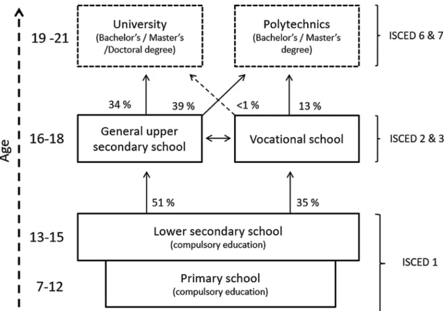
In Finland, the educational system is provided free of charge at all levels, including tertiary education, and studies are subsidized by student grants and subsidized student loans.Fig. 1provides an illustration of the Finnish educational system. Mandatory comprehensive school begins at age 7 and continues until age 15. The most significant transition occurs

after this period, when children apply for an academic (general upper secondary) or vocational track, each lasting approximately 3 years. Entry into the academic track is almost solely based on one’s GPA for the final year of comprehensive school. It is also possible to drop out after com-pleting compulsory education and not to continue with secondary edu-cation; however, only a small number of individuals choose to do so. In our dataset of cohorts for the period of 1986–1993, approximately 51 % attended general secondary school at age 16, approximately 36 % at-tended vocational secondary school and approximately 13 % did not continue to secondary-level schooling at 16 years of age.

After general secondary education, students often continue on to study at universities (mostly master’s level courses) or polytechnic schools (mostly bachelor’s level courses).Fig. 1shows that 34 % of the general secondary educated continued to universities and 39 % con-tinued to polytechnics. Thus, 27 % did not continue to tertiary-level studies from the general secondary level before they were 21 years old. From vocational secondary education, approximately 13 % continued to polytechnics and less than 1 % continued to universities. From vo-cational education, approximately 86 % did not continue to study at the tertiary level. For a more detailed account of early socioeconomic tra-jectories in Finland, seeKarhula, Erola, Raab, and Fasang (2019).

In the sample of cohorts born from 1986 to 1993, 17 % attended universities and 24 % attended polytechnics before they were 22 years old. In Finland, entry into universities and polytechnics is mostly based on entrance exams and in part on the matriculation exam of the general secondary education.

4. Data and methods 4.1. Register data

In the analyses, we use a register-basedFinnish Growth Environment dataset. The dataset is based on a 10 % sample of the Finnish

Fig. 1.Summary of the Finnish education system. Source: Ministry of Education and Culture 2015 and own calculations based on a sample of cohorts born 1986-1993. Note: ISCED 2011 classification.

population of 1980 that is matched with all the children born between 1986 and 1997. The dataset contains annual information on all applied variables from 1987 onwards so that we can observe parental un-employment yearly for every child. All persons are followed until 2014 or when they dropped out of the data because of either death or moving abroad. The analyses are restricted to biological siblings who lived in the same household with at least one biological parent (18.8 % of the children did not meet this condition). The children who started com-pulsory school one year before official age 7 (0.7 % of all children) and thus finished school one year before at the age of 14 are omitted from the analyses. The finalfull samplethat is applied in the random-effect models and therefore includes one-child families covers 113,100 in 79,151 families.

Our fixed-effects sample, which is used in the sibling fixed-effects models, is constructed in the following manner. First, we excluded singletons (N = 52,525) and twins in two-sibling families who lacked within family variation (N = 2108). Then, we omitted families in which children were not exposed to parental unemployment (N = 39,687), and we ultimately selected families in which the oldest sibling did not experience unemployment before his or her schooling was completed (a requirement for the control group), therefore excluding 16,272 cases. Thus, our final analytical sample for the fixed-effects models includes 2508 individuals in 951 families.

However, to study enrollment in tertiary education, we must be able to observe children who are older (at age 21) than for the two other outcomes (at age 15). Because of this, the data for these analyses are further restricted to the cohorts born between 1986 and 1993. In these analyses, the full sample includes 73.715 children in 53,821 families, and the fixed-effect sample includes 1855 children in 645 families. 4.2. Dependent and independent variables

We measure children’s educational achievement with the three different dependent variables:

1 Academic grade point average (GPA), based on the grades at the end of compulsory school, the year when children turn 15 (M = 7.68, SD = 1.05, Min = 4, Max = 10); the GPA is z-standardized for the analyses (M = 0, SD = 1).

2 Enrollment in general secondary school (ISCED 3) dummy variable at age 16 (M = 0.51).

3 Tertiary (ISCED-levels 6 and 7) educational enrollment dummy variable at ages 19–21 (M = 0.29).

These three different measurements give us the possibility of eval-uating how parental unemployment affects children’s schooling and thus distinguishes between the different mechanisms mentioned in the theory section. For example, grade point averages include grades for academic subjects that are evaluated when applied to the general sec-ondary school. Thus, the negative effect of parental unemployment on GPA indicates decreasing learning ambition, distraction, and cumula-tive effects, as predicted by our H2, which should be more evident in GPA than in more short-term choice-related outcomes, as indicated in the previous literature (Andersen, 2013). However, RRA should be limited to the entry into general secondary and higher education as predicted by H3a and H3b. RRA should be effective, especially before the transitional periods while controlling the grade point average (educational performance) and, in the case of tertiary education, sec-ondary school track choice (vocational or general secsec-ondary). This is because school performance can be a mediating factor behind the as-sociation between education decisions and parental unemployment.

Because the Finnish educational system is free of charge, we do not make assumptions about whether the impact of H1 on the economic ef-fects of parental unemployment applies differently across the outcomes.

Our main explanatory variable isage exposed to parental unemploy-ment for the first time. The previous research has shown that the negative

effects of parental unemployment on children’s school outcomes de-pend on the age when children experience it (Brand & Thomas, 2014). Furthermore, other disadvantageous life-course events, such as divorce (Grätz, 2015;Sigle-Rushton, Lyngstad, Andersen, & Kravdal, 2014) and poverty (Duncan & Brooks-Gunn, 2000), have also been shown to be dependent on a child’s age. Because all the siblings with a different year of birth experience parental unemployment at different ages (but in the same historical year), we can use this information in a sibling fixed-effect setup to identify the fixed-effect of parental unemployment on educa-tional outcomes. With our explanatory variable, we can study whether parental unemployment is disadvantageous for children’s education, and further, whether the negative effect is dependent on the child’s age when parental unemployment is experienced.

Parental unemployment is defined as either mothers’ or fathers’ un-employment. The auxiliary analyses (see Appendix Tables A.1a and A.1b in Supplementary material) show that there are no statistically significant differences in these effects in the Finnish context, although paternal un-employment seems to have stronger age-specific effects than maternal unemployment.1 _{We also provide histograms for the months of}

un-employment, as reported by mothers and fathers, in Appendix Fig. A.1 in Supplementary material. The histograms show very similar distributions. The information on unemployment is based on the number of months a parent has been registered as unemployed in employment offices within a single year. A parent is defined as unemployed if un-employment continues for more than one month during a year. Some of the previous studies have applied a less strict limit of 4–5 months (see Eghaugen, 2009) to exclude parents with short transitory periods of unemployment. In our case, the results do not change substantively if similar limit is applied in our analyses, although many fewer parents fall into the group of unemployed, which also subsequently broadens the confidence intervals (see results Appendix Table A.2a compared to Table A.5 in Supplementary material).

Due to the unemployment benefits received if registered, the un-derreporting of unemployment is rare. However, we are not able to observe whether unemployment is voluntary or involuntary, and this should be noted when interpreting the results. If our sample contained parents, who are voluntarily unemployed, this would lead to an un-derestimation of the results; however, this is hardly the case. A study that examined voluntarily based unemployment in Finland concluded that only 1 % can be considered to be voluntarily unemployed of all the unemployed (Martikainen, 2003). This share is likely to be even lower among the unemployed parents studied here. Because unemployment may have detrimental effects on health, we exclude the parents who were unemployed due to a disability.

In random intercept models, we can differentiate the effects based on each age of experiencing parental unemployment for the first time, starting from age 1. However, in the sibling fixed-effect models, sin-gletons and children who are not exposed to unemployment must be excluded from the analyses, which limits the number of cases con-siderably. Consequently, there are only a few cases left in which par-ental unemployment was experienced during early childhood. Therefore, in the models forGPAandgeneral secondary enrollment,we combine all those experiencing parental unemployment before age eight into one group.2_{In addition, because the number of cases was also}

too low when we modeled ages 8–10 individually, we combine ages 8–10 into same group. The separate effects for each age are differ-entiated from those experiencing unemployment at ages 11–15 while

1_{The differences of the effects and the point estimates of maternal and} pa-ternal unemployment on children’s education outcomes are discussed further in the additional analyses.

2_{Note that the gains in statistical power following from this are not as great} as they would be in random intercept models. To observe any effects, siblings must fall under different age categories; however, sample consists only few families in which siblings’ ages differ by 9 years or more.

keeping as a reference group siblings who did not experience parental unemployment by age 15 and those who finished their compulsory schooling.

In the models fortertiary education enrollment, we limit our analyses to those who continue their education to at least secondary education. Children finish compulsory school at age 15, and those not continuing to secondary education cannot continue to tertiary education. Further, in these models, we differentiate age-specific effects with four dummy indicators, one each for age 15 and younger to age 18. Further, children typically finish their secondary education by age 19, and it is relatively usual to have left the parental home for good by that age (35 % ac-cording to official statistics). Eghaugen (2009) used a similar upper-age cut-off point previously.

In the sibling fixed-effect models, we are unable to control the parental educational level because it is a constant among siblings. To compare the results by the level of parental education, we must run separate sets of models according to them. To do so, we distinguish two levels of parental education: (I) Compulsory or vocational degree, (II) Academic track degree (general secondary degree or higher).

The information on parental education is acquired from the same or the closest earlier year when one of the parents experienced employment. For those children who did not experience parental un-employment, included in our random-effect models only, we take the highest level of education of either parent by age 19.3_{We distinguished}

only two levels of parental education to gain maximum statistical power for the sibling fixed-effect models.4_{Table 1(see4.5Descriptive}

statistics) shows the descriptive statistics of parental education sepa-rated into six categories, which are used as the control variables in the random-effect models.

4.3. Control variables

We control for the set of variables between siblings that are asso-ciated with children’s educational achievement and parental un-employment. Our baseline sibling fixed-effect models control for the child’s sex, year of birth, siblings’ birth orderandduration of parental un-employmentin months. All of these factors vary between siblings and have been shown to affect educational achievement (e.g., Andersen, 2013;Brand & Thomas, 2014;Ekhaugen, 2009;Härkönen, 2014; Sigle-Rushton et al., 2014). The auxiliary analyses (see Appendix Table A.2b in Supplementary material) show that the duration of parental un-employment is not statistically significant for the outcomes. However, the duration of unemployment can play a role, albeit relatively modest, in the sibling fixed-effect models where we investigate age exposed to parental unemployment; consequently, we decided to control for it. Additionally, in random intercept models, we control for maternal and paternal education including six categories (see descriptive statistics) and family type (intact or non-intact family) during parental un-employment that is constant between siblings.

The baseline fixed-effect models—where we control for the child’s sex, birth year, siblings’ birth order and duration of parental un-employment—are compared to the additional models used to test our hypotheses. In the models for entry into general secondary- and tertiary education, we control for the grade point averages of the academic subjects and provide a dummy indicator if those data are missing (3 %).

Thus, we can analyze whether school performance mediates the effects of parental unemployment and education enrollment. If a person has not applied to any secondary education program after finalizing com-pulsory education, the GPA is never centrally registered. Additionally, the GPA is missing for a very small number of children because they never finalized their compulsory schooling (approximately one in 250 by official statistics).

Further, we control for average annual family income. The annual family income is calculated by taking the total gross income of the parents living in the same household with a child, which is then de-flated to the price level of the year 2014 and log-transformed. When estimating the models for GPA and secondary education enrollment, the average annual family income is based on the total family income of a child by the age of 15; for tertiary enrollment, it is based on the total family income of a child by the age of 18. We are not able to calculate net family income (income after taxes) for every follow-up year because the tax registers that we use do not contain tax records before the year 1991; thus, in the analyses, we use gross family income (income before taxes).

In the models, where we analyze tertiary enrollment by parental education, we also control for children’s secondary school selection (whether they enroll in general or vocational secondary schools) and GPA to study the relative risk-aversion mechanism.

4.4. Methods

One of the obvious problems in studying the association between parental unemployment and children’s later attainment is selection bias. Unemployment is not a random event; however, individuals with other disadvantageous characteristics are likely to select into un-employment. Thus, confounding factors may be behind the relationship between parental unemployment and children’s educational achieve-ment. If these factors are unobservable, the direct effect of unemploy-ment cannot be observed even if the association is found. Selection bias can lead to overestimation of the negative effect or, even worse, erro-neous conclusions about the relationship between parental unemploy-ment and children’s educational achieveunemploy-ment.

In this study, we use a register-based dataset that contains in-formation about parents and their children within families, thus, we are able to employ sibling fixed-effect models to control for the potential bias caused by unobserved confounding factors. This means that any family background-related effects shared by siblings, observed or un-observed, are controlled for in the models. Thus, our models yield fewer biased estimates than regular (between-individual) regression esti-mates. By controlling for unobserved confounding variables at the fa-mily level, the sibling fixed-effect technique reduces the unobservable heterogeneity problem and can be seen to more accurately reflect the causal relationship between independent and dependent variables (see, e.g.,Sigle-Rushton et al., 2014). A similar approach has previously been used to study the intergenerational effects of unemployment (Ekhaugen, 2009) and divorce (Sigle-Rushton et al., 2014).

The sibling fixed-effect model has been considered a simple exten-sion of the matched case-control design. All the effects that are being estimated are those that differentiate siblings from one another. In our setup, the most important of such factors is the age when each sibling experiences parental unemployment.

Siblings with different year of birth experience parental unemploy-ment periods at different ages but within the same year. We can use this information in a sibling fixed-effect design to identify the effect of parental unemployment on educational outcomes. In the models, the oldest siblings are assigned to our reference (or control) group. They experience parental unemployment only after compulsory or secondary school is finished. Thus, only the later born siblings (treatment group) are exposed to par-ental unemployment before they finish their schooling.

Sibling fixed-effect models automatically control for any measured or unmeasured factors shared by siblings at the family level. In our case,

3_{Because either mothers or fathers can be unemployed, we also tested models} with combinations of parental education. We do not find statistically significant differences, as reported in the results section.

4_{While we also created models adopting different categorizations of parental} education, the categorizations used here provide the highest levels of statistical fit and power. For example, when we categorized highly (tertiary) and less educated parents (those with a general secondary education were included in this group) into separate groups, the estimates remained the same, as the sta-tistical power decreased for the highly educated parents while the sibling FE-models assigned less statistical significance to the estimates.

these unobserved factors are a family’s shared cultural capital; parental characteristics, such as education, child-rearing practices (if the same for all siblings); neighborhood effects; and genetic variance that siblings share (Frisell, Öberg, Kuja-Halkola, & Sjölander, 2012).

In sibling fixed-effect models, children are nested into their families. We use linear probability models to estimate the average marginal ef-fects of general secondary and tertiary enrollment and linear models for the estimates of the grade point averages. We compare the estimates from the sibling fixed-effect models with the results from random in-tercept models to show how much unobservable heterogeneity con-tributes to the estimates, because the random intercept model does not control for all family-level factors and thus does not take into account all unobserved heterogeneity. In the sibling fixed-effect models, we use a robust standard errors estimator. Eq.(1)shows how the sibling fixed-effect model is estimated, and Eq.(2)shows how the random intercept model is estimated.

= + + +

Yfi Xfi Zfi af efi (1)

= + + + + +

Yfi 0 Xfi Zfi f uf efi (2)

Here,f refers to a family, andirefers to a sibling. The vector Xfiis a set of dummy variables of parental unemployment at a certain age of the sibling, Z_firefers to the vector of sibling-specific control variables, and

f refers to family-level control variables (only in random-effect

models). In the fixed-effect model, f is the family-specific intercept,

which is constant between siblings controlling all factors that are in-variant on the family level.efiis the within-sibling error term (variation

between siblings).

Although sibling fixed-effect models are an efficient method to control for omitted variable bias at the family level, they also have certain limitations. First, the models do not automatically control any confounding factors that vary between siblings but are not included in the model. Second, sibling fixed-effect models can only be estimated among families with at least two children. Thus, one-child families have omitted from the sibling fixed-effect models. Third, sibling fixed-effect models cannot control for reverse causality. For example, a child’s poor health or the birth of a younger sibling may affect a parent’s decision to become unemployed. By including certain sibling-specific control variables such as a child’s year of birth, siblings’ birth order, family income and grade point averages, some of these problems can be at least partially overcome (see, e.g.,Sigle-Rushton et al., 2014).

4.5. Descriptive statistics

The descriptive statistics of the full and fixed-effect samples in Table 1show that our dependent and independent variables are close to each other in both samples. The only variables that differ significantly are those for the age of exposure to parental unemployment. In the analytical fixed-effect sample, the average age of exposure is higher because the oldest sibling must be either over 15 or 18 (depending on the outcome), and thus the younger siblings are exposed to parental unemployment on average somewhat older.

We test the potential selection bias of the fixed-effect sample by comparing the estimates from a set of OLS regression models run for both samples and for all outcomes. The estimates for independent variables are reported in the Appendix Tables A.3a and A.3b in Supplementary material. The tables also show Wald tests for the dif-ferences between fixed-effect and total sample estimates. We find that the results for the two samples differ significantly statistically for only a single estimate of GPA. The estimate for vocationally educated mothers is effectively zero in the fixed-effect sample but positive and statistically significant in the total sample. The comparison indicates that the fixed-effect sample does not suffer from selection bias.

5. Results

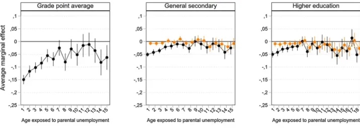
We begin the results section by showing the average effects of parental unemployment by children’s age on each outcome. We use the full sample to estimate the random-effect results and the fixed-effect sample in the sibling fixed-effect models.Fig. 2shows the results of the random-effect models andFig. 3of the sibling fixed-effect models by children’s age when exposed to parental unemployment, with baseline controls. When the dependent variable is general secondary or tertiary education enrollment, we also control for GPA to check whether the children’s school performance explains educational choices. All the estimates are reported in the Appendix Tables A.4a and A.4b in Sup-plementary material for RE models and Table A.5 for FE models. In both Figures, 95 % confidence intervals are displayed around the estimates. For GPA, the random-effects results inFig. 2show that parental unemployment is the most disadvantageous to children’s education if it is experienced in early childhood, reducing children’s GPA on average 0.15–0.055 standard deviations at age 1–5, and again just before the end of compulsory schooling at age 14–15 (the average point estimate is between −0.06 and −0.08). In the case of general secondary and tertiary enrollment, the experience of parental unemployment shows a very similar pattern. From ages 1–5, children who experience parental unemployment have, on average, a 2–5 percentage points lower prob-ability of enrolling in general secondary or tertiary education than children who do not experience parental unemployment. Again, at age 14, parental unemployment reduces general secondary enrollment by an average of 4 percentage points and tertiary enrollment by an average of 5 percentage points. Furthermore, exposure to parental Table 1

Descriptive statistics of applied variables.

Full sample FE sample

VARIABLES Mean Sd. Mean Sd. Within Sd. Tertiary enrollment 0.29 0.46 0.3 0.46 0.33 General secondary enrollment 0.51 0.5 0.51 0.5 0.32 Academic GPA 7.68 1.08 7.72 1.05 0.64 Standardized academic GPA 0 1 0.03 0.97 0.6 GPA missing 0.03 0.17 0.03 0.17 0.10 Female 0.49 0.5 0.48 0.5 0.40 Year born 1991 3.46 1991 3.25 2.41 Birth order 1.97 1.28 2.64 2.08 0.92 Age at parental unemployment

(until 15)a 2.61 3.49 6.53 6.74 6.52

Age at parental unemployment

(until 18)a 3.13 4.25 12.45 5.72 4.48

Duration of parental

unemployment (1–15) 21.01 32.66 3.92 7.89 6.11 Duration of parental

unemployment (1–18) 23.6 36.32 8.75 11.91 7.12 Log of family income 10.85 0.53 10.98 0.48 0.14 Vocational secondary enrollment 0.39 0.49 0.42 0.49 0.33 Parental separation 0.18 0.38 0.19 0.39 NA. F. Basic education 0.2 0.4 0.16 0.37 NA. F. Vocational secondary 0.42 0.49 0.4 0.49 NA. F. General secondary 0.07 0.25 0.04 0.19 NA. F. Postsecondary 0.13 0.34 0.16 0.37 NA. F. Tertiary: bachelor's degree 0.08 0.28 0.12 0.32 NA. F. Tertiary: master's degree or

higher 0.1 0.31 0.12 0.33 NA. M. Basic education 0.15 0.36 0.09 0.29 NA. M. Vocational secondary 0.38 0.48 0.4 0.49 NA. M. General secondary 0.08 0.27 0.05 0.21 NA. M. Postsecondary 0.22 0.41 0.26 0.44 NA. M. Tertiary: bachelor's degree 0.08 0.27 0.08 0.28 NA. M. Tertiary: master's degree or

higher 0.1 0.3 0.11 0.31 NA.

N 113100 2508

NA. = not applicable.

unemployment at age 18 decreases the probability of enrollment in tertiary education by 5 percentage points. In general, children who experience parental unemployment have a 2–5 percentage points lower probability of enrolling in general secondary or tertiary education.

The associations should be considered to be relatively weak for all three outcomes, The results are also in line with the previous research, also showing that parental unemployment reduces by approximately 5 percentage points postsecondary enrollment in Finland, and among European countries, the effect is one of the smallest (seeLindemann & Gangl, 2018). Finally, when we control for GPA in the models the ne-gative association of parental unemployment with general secondary education, entry becomes negligible, and the effects on tertiary en-rollment become very small (3.5 percentage points or less).

Overall, the random-effect models indicate that parental un-employment experienced in early childhood is disadvantageous, parti-cularly for children’s GPA, indicating the importance of Hypothesis 2 with regard to cumulative effects. Further, parental unemployment is disadvantageous at an age when educational choices are still made after controlling the GPA for tertiary enrollment, indicating a higher risk of

continuing in tertiary education among children who are exposed to unemployment, thus supporting Hypotheses 3a and 3b. However, be-cause the random-effect models do not entirely control for the un-observed heterogeneity at the family level, we must compare the results to the sibling fixed-effect models.

The results of sibling fixed-effect models inFig. 3show a different pattern for GPA, asFig. 2for the random-effect models. Parental un-employment is not detrimental in early childhood when children are 7 years old or younger; however, it is at the ages of 14 and 15. Parental unemployment reduces treated siblings’ GPA on average with a stan-dard deviation of 0.13–0.17. Because error terms (and confidence in-tervals) are much larger in sibling fixed-effect models, age differences are not statistically significant.

For general secondary enrollment, the negative effect of parental unemployment is found at the end of compulsory education when the treated siblings are 13–14 years old. Thus, parental unemployment again has a negative effect at the end of compulsory school. Parental unemployment decreases the probability of enrolling in general sec-ondary school by on average 10 percentage points. This is also true for Fig. 2.The estimated effect of parental unemployment on children’s GPA (left panel), general secondary enrollment (middle panel), tertiary enrollment (right panel) using random intercept models and average marginal effects. Note: Baseline models (black symbols) control for year of birth, birth order, child’s sex, duration of parental unemployment, maternal and paternal education and family type. Orange symbols control for baseline model’s variables and GPA. 95 % confidence intervals around the estimates.

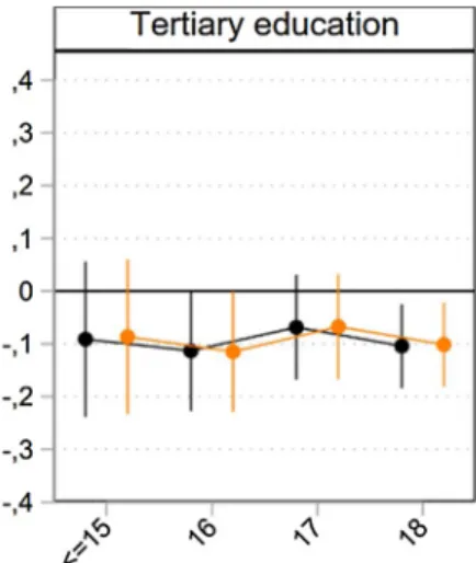
Fig. 3.The estimated effect of parental unemployment on children’s GPA (left panel), general secondary enrollment (center panel), tertiary enrollment (right panel) using sibling fixed-effects models, and average marginal effects. Note: Black symbols (baseline models) control for year of birth, birth order, child’s sex, duration of parental unemployment. Orange symbols control for baseline model’s variables and GPA. 95 % confidence intervals around the estimates.

tertiary enrollment. The negative effect of the treatment group can be observed at the very end of secondary school when children are age 18. Parental unemployment reduces the probability of enrolling in tertiary education by on average 12 percentage points. As with secondary en-rollment and GPA, this can again be observed at the age when further education choices are made.

When we control for GPA, the negative effect disappears entirely in the case of entry into general secondary education. In the case of ter-tiary education enrollment, the negative effect also decreases; however, the difference remains statistically and substantively significant, on average at 10.6 percentage points between the treatment and control groups. The previous studies have also reported the negative causal effect of parental unemployment on children’s tertiary enrollment to be on average 10 percentage points in the US and Canada (Brand & Thomas, 2014; Coelli, 2011); however, in Germany, it is on average somewhat higher at 13 percentage points (Lindemann & Gangl, 2019). We can conclude that for all three outcomes, parental unemploy-ment is disadvantageous at the age when children are adolescents and understand the meaning of parental unemployment. This is also a time when children are at the end of compulsory education and when further education decisions are made. In our analysis, parental unemployment is not significantly detrimental in early childhood, the life-course stage when children’s emotional and cognitive skills are still developing. However, our estimates at those ages have relatively large confidence intervals, and the lack of statistical power makes these conclusions less certain. Furthermore, the negative effect of parental unemployment for secondary enrollment is explained by lower school performance. However, school performance in compulsory education does not ex-plain the negative effect of parental unemployment on tertiary enroll-ment at age 18. The results for GPA (and enrollenroll-ment outcomes) also indicate that the negative effects of experiencing parental unemploy-ment in early childhood in random-effects models are explained by the selection into unemployment and not by the causal effect of un-employment on children. Thus, fixed-effects models do not support Hypothesis 2 regarding the cumulative effects of parental unemploy-ment with respect to age.

5.1. The mediating effects of family income

Next, we analyze whether family income explains the negative ef-fect of parental unemployment on children’s educational achievement as predicted by our Hypothesis 1. Because we found above that parental unemployment does not affect general secondary enrollment, these

analyses are conducted only for GPA and tertiary enrollment. Fig. 4shows how much controlling for differences in family income between treatment and control groups influences the negative effect of parental unemployment. The left-hand panel shows that family income is not related to the negative effect in the case of GPA - the black and orange lines overlap. The same can be observed for tertiary enrollment in the right-hand panel: family income does not explain the differences between siblings. In addition, the estimates for family income are small and not statistically significant (see Table A.6 in the Appendix in Sup-plementary material).

As a robustness check, we conducted the same analyses by splitting the incomes into deciles and including each decile into the models as dummy variables to test whether there are nonlinearities in the effects of family income. We found no mediating effect of family income in this analysis either (results available from the authors upon request). Finally, we conducted additional analyses by controlling for family income specifically at age 14–15 for GPA and at age 18 for tertiary education, which are the ages for which we found a negative effect of parental unemployment (see Appendix Table A.6b in Supplementary material). The results remained the same; we did not find any med-iating effects of family income.5_{Thus, we concluded that family income}

did not mediate the negative effect between parental unemployment and children’s education. It should be noted that we used family income as measured before taxes. With other measures, the results may change; unfortunately, we did not have access to data for values measured after applying taxes and subsidies. With income being measured before tax, we underestimate the incomes of poor families receiving subsidies and overestimate the incomes of single-earner families, as the income tax system is progressive, and based on individual earnings. Overall, this may create slight biases in the analysis, but we expect these to be re-latively minor.

5.2. Parental education

Finally,Table 2shows the effects of parental unemployment ac-cording to parental education level. In the table, we distinguish two education levels for parents: parental education low is for siblings whose parents have vocational or lower education, and parental Fig. 4.The estimated effects of parental un-employment on children’s GPA (left panel) and tertiary enrollment (right panel) without and with controlling for family income using sib-ling fixed-effects models and average marginal effects. Note: Black symbols (baseline models) control for year of birth, birth order, child’s sex, duration of parental unemployment and for tertiary enrollment GPA. Orange symbols control for baseline model’s variables and fa-mily income. 95 % confidence intervals around the estimates.

5_{We also conducted sensitivity analyses controlling family incomes before} the age at which a child is exposed to parental unemployment and during the exposure age. However, the results remained the same.

education high is for the siblings whose parents have general secondary or higher education. In these models, we also control for family income. The purpose of these analyses is to further study whether higher edu-cated parent’s unemployment increases time discounting preferences in tertiary education enrollment as predicted by Hypotheses 3a and 3b, and/or whether higher parental education compensates the negative effects of unemployment as predicted by Hypothesis 4.

In the first two models, our outcome variable is children’s GPA. These models show that only the children of lower educated parents are statistically significantly affected by parental unemployment at ages 12 and 14. The next two models are for general secondary education; again, parental unemployment has a statistically significant negative effect on siblings’ general secondary enrollment among lower educated parents but not higher educated parents at ages 13–14. These findings support Hypothesis 4 that higher parental education protects children from the negative effects of parental unemployment. However, one should note that differences between the point estimates are not sta-tistically significant, and thus we cannot definitively conclude the presence of differences between lower and higher levels of parental education.

However, in the next two models, which are for tertiary enrollment, we do find that parental unemployment has a detrimental effect among higher educated parents at age 18. This may indicate higher perceived risks in continuing tertiary education.

To test this further, we conducted analyses for tertiary enrollment where we controlled both GPA and education choice after compulsory school (whether the children were enrolled in the general secondary- or vocational education). The previous research indicates that, in Finland, children with advantageous educational family backgrounds have a higher probability of enrolling in the general secondary track than children do from disadvantageous educational backgrounds ( Kilpi-Jakonen, Erola, & Karhula, 2016).

Table 3shows the results when we control for GPA (model 1) and school selection (model 2) between siblings. As in the previous models inTable 2, we do not find any statistically significant estimates among siblings with lower educated parents in these models. However, we find a significant and substantial negative effect (on average 15 percentage points) among the siblings with higher educated parents when a child is 18 years old, during the last year of general secondary education, even when we control for both GPA and school selection (whether children choose vocational- or general secondary school) in model 2. However, the above mentioned differences between estimates for lower and higher levels of parental education are not statistically significant.

GPA differences and school selection between siblings among chil-dren from higher educated families do not explain away the negative effect of parental unemployment. This finding indicates that the chil-dren of better-educated parents are less likely to apply to tertiary education when they experienced parental unemployment at the very Table 2

The estimated effects of parental unemployment on children’s educational outcomes according to parental education level. Sibling fixed-effects models, average marginal effects.

GPA General secondary Tertiary

1 2 1 2 1 2

Par edu low Par edu high Par edu low Par edu high Par edu low Par edu high Age exposed to parental unemployment (ref. No unemployment)

≤7 −0,364 0,484 −0,167 0,328 0,5 0,304 0,246 0,191 8–10 −0,462 0,165 −0,212 0,046 0,245 0,177 0,126 0,108 11 −0,29 0,006 −0,009 −0,004 0,212 0,167 0,128 0,098 12 −0,404* 0,032 −0,138 0,045 0,204 0,13 0,09 0,084 13 −0,161 −0,143 −0,133 −0,078 0,139 0,113 0,073 0,071 14 −0,304* −0,094 −0,136* −0,061 0,125 0,096 0,065 0,055 15 −0,182 −0,085 −0,062 −0,037 0,114 0,078 0,055 0,049 < 15 −0,107 −0,02 0,125 0,118 16 0,098 −0,142 0,105 0,094 17 −0,024 −0,059 0,08 0,082 18 −0,066 −0,152* 0,061 0,066 Female 0,577*** 0,565*** 0,181*** 0,202*** 0,023 0,172*** 0,062 0,047 0,034 0,025 0,042 0,039

family income (log) 0,04 0,231 −0,108* 0,208 0,04 0,085

0,058 0,199 0,047 0,138 0,202 0,246 Duration of unemploymenta _{0,004 −0,004 0,004 0,001 0,003 0} 0,004 0,003 0,002 0,002 0,005 0,006 Year born 0,016 0,023 −0,023 −0,021 −0,032 −0,027 0,031 0,023 0,015 0,013 0,021 0,021 Birth order −0,024 −0,095* 0,048 0,002 0,051 0,013 0,061 0,041 0,025 0,024 0,041 0,046 GPA missing 0,286 −0,350* 0,162 0,163 BIC 1641,419 2583,136 490,53 823,675 142,588 450,559 N 927 1581 927 1581 730 1127

Standard errors in second row *p< 0.05, **p< 0.01, ***p< 0.001.

end of their secondary education careers or at the point of determining whether to prepare for entry exams for tertiary education programs. This supports Hypothesis 3a that the negative effect of parental un-employment on children becomes stronger as the parental level of education increases and Hypothesis 3b that the effect of parental un-employment is more detrimental just before educational transition periods.

Children with different levels of parental education might experi-ence different selection processes upon entry to secondary education. The children with low parental education entering the general sec-ondary track may have higher abilities on average than the children of highly educated parents, and this pattern, in turn, could bias the esti-mates of low and high parental education. We control for GPA at the end of primary school to account for this kind of selection, but un-related selection might still exist. However, we believe that such a complex selection is unlikely to cause significant bias.

5.3. Additional analyses

Because our analysis also covers children who experienced parental separation before parental unemployment (approximately 19 % of the cases in the fixed-effect models), and the parents who were unemployed in the household were not always biological parents in our analyses, we conduct sensitivity analyses only for the cases where there were intact two-biological-parent families. In these analyses, we do not find any significant differences from the results reported above (see Appendix Table A.7a in Supplementary material). Further, Appendix Table A.7b in Supplementary material shows the estimates for the interaction be-tween family type and exposure to parental unemployment without differentiating the age of exposure. The results from the Wald test show significant interaction when the outcome is GPA; however, the main

effect is significant for both intact and nonintact families but the coefficient is stronger for siblings who live in nonintact families when they experience parental unemployment. For enrollment outcomes, we do not find significant interaction terms between intact and nonintact families.

We also tested interactions between the sex of a child and age at parental unemployment. The analyses reported in Appendix Tables A.8a–A.8c in Supplementary material indicate that the effects of par-ental unemployment do not substantially differ between sons and daughters. The only interaction effect that we found to be significant was for GPA at age 15, when parental unemployment was only detri-mental for sons but not for daughters. This indicates that there are only minor differences between sons and daughters.

Although we do not find any major differences between the effects of parental unemployment for sons and daughters, the analyses show significant negative effects for daughters but not for sons at age 18 when the outcome variable is tertiary enrollment. When the outcome variable is general secondary enrollment, we find a significant negative effect for sons but not for daughters at age 15. For general secondary enrollment, the effects are also marginally significant (p < 0.10) for both sons and daughters at the age of 14, and for sons at age 13. For GPA, we find that the effects are significant for sons at age 14 and marginally significant at ages 12 and 13.

However, the results of these analyses must be interpreted with caution because the error term grows rather large due to a lack of statistical power. To obtain more power, we conducted similar gender-interaction analyses without differentiating the age of exposure to specific effects, thus comparing those experiencing parental un-employment to those who do not (see Appendix Table A.9 in Supplementary material). For GPA, the effect of sons is somewhat stronger, and we also find marginally significant interaction; however, the main effect of daughters is also marginally significant but smaller. For secondary enrollment, we find significant effects for sons and marginally significant effects for daughters, but no significant interac-tion effect. For tertiary educainterac-tion enrollment, we find significant main effects for daughters, but no significant interaction effects. Thus, we cannot argue that parental unemployment is detrimental only for daughters or sons, but most likely it is detrimental for both.

Because there can be differences between the effects of paternal or maternal unemployment, we conducted separate analyses for the fa-milies in which siblings experience only maternal or paternal un-employment. The results reported in Appendix Tables A.1a and A.1b in Supplementary material show no statistically significant differences between the effects of maternal and paternal unemployment (con-fidence intervals overlap).

Although confidence intervals overlap, paternal unemployment seems somewhat more disadvantageous for children’s GPA at ages 11 and 14. Additionally, only paternal unemployment is significant for tertiary enrollment at ages 16–18. Paternal unemployment is also sig-nificant for general secondary enrollment at ages 13–14, although it is not statistically significantly different from maternal unemployment. Thus, it seems that paternal unemployment is somewhat more dis-advantageous for children’s school performance and education selec-tion than maternal unemployment at certain ages.

We also conducted these analyses without differentiating age-specific effects (see Appendix Table A.1b in Supplementary material), and the findings provide more support for our conclusion that there are some differences between the effects of mothers’ and fathers’ unemployment for tertiary enrollment. In Appendix Table A.1b in Supplementary material, the point estimate of paternal unemployment for tertiary enrollment is lower (and thus on average has a greater effect) than maternal un-employment, and the difference between effects is statistically significant. This finding supports status deprivation, which increases children’s per-ceived risks in enrolling in tertiary education because fathers have higher occupational status and they are usually affected more by unemployment than mothers (see, e.g.,Andersen, 2013).

Table 3

The estimated effects of parental unemployment on children’s tertiary educa-tion enrollment according to parental educaeduca-tion level when adjustments are made for GPA and education selection. Sibling fixed-effects models, average marginal effects.

Par edu low Par edu high Par edu low Par edu high Age exposed to par unemployment (ref. No unemployment)

< 15 −0.107 −0.057 −0.123 −0.059 0.101 0.1 0.095 0.099 16 0.016 −0.179* 0.033 −0.151 0.079 0.082 0.08 0.083 17 −0.076 −0.051 −0.067 −0.037 0.077 0.066 0.071 0.066 18 −0.034 −0.146** −0.032 −0.147** 0.056 0.057 0.054 0.057 Female −0.097** −0.022 −0.085** −0.042 0.04 0.039 0.038 0.038 Year of birth −0.018 −0.018 −0.014 −0.002 0.019 0.02 0.019 0.02 Birth order 0.033 0.036 0.031 0.051 0.034 0.043 0.033 0.041 Duration of parental unemploymenta 0.004 0.002 0.005 0.001 0.003 0.005 0.003 0.005

log family income 0.237 0.094 0.166 0.017

0.17 0.226 0.156 0.22 GPA 0.233*** 0.263*** 0.163*** 0.215*** 0.025 0.027 0.024 0.03 GPA missing −0.149 −0.400* 0.038 −0.35*** 0.101 0.11 0.125 0.062 Vocational enrollment (ref. General sec) −0.231*** −0.204*** 0.049 0.046 BIC 13.951 235.874 −36.047 204.245 N 730 1127 730 1127

Standard errors in second row *p< 0.05, **p< 0.01, ***p< 0.001. a _{Duration of parental unemployment is calculated until children were 18.}