A Unified Theory of Tobin’s
q
, Corporate
Investment, Financing, and Risk Management
PATRICK BOLTON, HUI CHEN, and NENG WANG∗
ABSTRACT
We propose a model of dynamic investment, financing, and risk management for financially constrained firms. The model highlights the central importance of the en-dogenous marginal value of liquidity (cash and credit line) for corporate decisions. Our three main results are: (1) investment depends on the ratio of marginalqto the marginal value of liquidity, and the relation between investment and marginal
qchanges with the marginal source of funding; (2) optimal external financing and payout are characterized by an endogenous double-barrier policy for the firm’s cash-capital ratio; and (3) liquidity management and derivatives hedging are complemen-tary risk management tools.
WHEN FIRMS FACE EXTERNALfinancing costs, they must deal with complex and
closely intertwined investment, financing, and risk management decisions. How to formalize the interconnections among these margins in a dynamic setting and how to translate the theory into day-to-day risk management and real investment policies remains largely to be determined. Questions such as how corporations should manage their cash holdings, which risks they should hedge and by how much, or the extent to which holding cash is a substitute for financial hedging are not well understood.
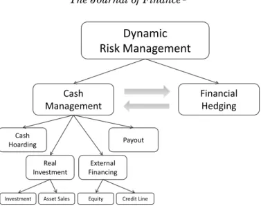
Our goal in this article is to propose the first elements of a tractable dy-namic corporate risk management framework—as illustrated in Figure 1—in which cash inventory, corporate investment, external financing, payout, and dynamic hedging policies are characterized simultaneously for a “financially constrained” firm. We emphasize that risk management is not just about fi-nancial hedging; instead, it is tightly connected to liquidity management via ∗Bolton is at Columbia University, NBER, and CEPR. Chen is at MIT Sloan School of
Man-agement and NBER. Wang is at Columbia University, NBER, and Shanghai University of Fi-nance & Economics. We are grateful to Andrew Abel, Peter DeMarzo, Janice Eberly, Andrea Eisfeldt, Mike Faulkender, Michael Fishman, Xavier Gabaix, John Graham, Dirk Hackbarth, Cam Harvey, Christopher Hennessy, Pete Kyle, Yelena Larkin, Robert McDonald, Stewart My-ers, Marco Pagano, Gordon Phillips, Robert Pindyck, Adriano Rampini, David Scharfstein, Jiang Wang, Toni Whited, two anonymous referees, and seminar participants at Boston College, Boston University, Columbia Business School, Duke, MIT Sloan, NYU Stern and NYU Economics, Uni-versity of California at Berkeley, Yale, Maryland, Northwestern, Princeton, Lancaster, Virginia, IMF, Hong Kong University of Science and Technology Finance Symposium, Arizona State Univer-sity, American Finance Association Meeting, the Caesarea Center 6th Annual Academic Confer-ence, European Summer Symposium on Financial Markets, and Foundation for the Advancement of Research in Financial Economics for their comments.
Figure 1. A unified framework for risk management.
daily operations. By bringing these different aspects of risk management into a unified framework, we show how they interact with and complement each other.
The baseline model we propose introduces only the essential building blocks, which are: (i) the workhorse neoclassical q model of investment1 featuring
constant investment opportunities as in Hayashi (1982); (ii) constant external financing costs, which give rise to a corporate cash inventory problem as in Miller and Orr (1966); and (iii) four basic financial instruments: cash, equity, line of credit, and derivatives (e.g., futures). This parsimonious model already captures many situations that firms face in practice and yields a rich set of prescriptions.
With external financing costs, the firm’s investment is no longer determined by equating the marginal cost of investing with marginal q, as in the neo-classical Modigliani and Miller (1958; MM) model (with no fixed adjustment costs for investment). Instead, investment of a financially constrained firm is determined by theratio of marginal q to the marginal cost of financing:
marginal cost of investing= marginalq
marginal cost of financing.
When firms are flush with cash, the marginal cost of financing is approximately one, so that this equation is approximately the same as the one under MM. But
1Brainard and Tobin (1968) and Tobin (1969) define the ratio between the firm’s market value and the replacement cost of its capital stock as “Q” and propose that this ratio be used to measure the firm’s incentive to invest in capital. This ratio has become known as Tobin’s averageQ. Hayashi (1982) provides conditions under which averageQis equal to marginalq. Abel and Eberly (1994) develop a unifiedqtheory of investment in neoclassic settings. Lucas and Prescott (1971) and Abel (1983) are important early contributions.
when firms are close to financial distress, the marginal cost of financing, which is endogenous, may be much larger than one so that optimal investment may be far lower than the level predicted under MM. A key contribution of our article is to analytically and quantitatively characterize the marginal value of cash to a financially constrained firm as a function of the firm’s investment opportunities, cash holding, leverage, external financing costs, and hedging opportunities.2
An important result that follows from the first-order condition above is that the relation between marginal q and investment differs depending on whether cash or credit is the marginal source of financing. When the marginal source of financing is cash, both marginal q and investment increase with the firm’s cash holdings, as more cash makes the firm less financially con-strained. In contrast, when the marginal source of financing is the credit line, we show that marginalqand investment move in opposite directions. On the one hand, investment decreases with leverage, as the firm cuts investment to delay incurring equity issuance costs. On the other hand, marginal q in-creases with the firm’s leverage, because an extra unit of capital helps relax the firm’s borrowing constraint by lowering the debt-to-capital ratio, and this effect becomes increasingly more important as leverage rises. Thus, there is no longer a monotonic relation between investment and marginalq in the pres-ence of a credit line, and averageqcan actually be a more robust indicator for investment.
A second key result concerns the firm’s optimal cash inventory policy. Much of the empirical literature on firms’ cash holdings tries to identify atarget cash inventory for a firm by weighing the costs and benefits of holding cash.3 The idea is that this target level helps determine when a firm should increase its cash savings and when it should dissave.4Our analysis, however, shows that
the firm’s cash inventory policy is much richer, as it involves a combination of a double-barrier policycharacterized by a single variable, the cash-capital ratio, and the continuous management of cash reserves in between the barriers through adjustments in investment, asset sales, as well as the firm’s hedging positions. While this double-barrier policy is not new (it goes back to the inven-tory model of Miller and Orr (1966) in corporate finance), our model provides substantial new insight on how the different boundaries depend on factors such as the growth rate and volatility of earnings, financing costs, cash holding costs, as well as the dynamics of cash holdings in between these boundaries.
2Hennessy, Levy, and Whited (2007) derive a related optimality condition for investment. As they assume that the firm faces quadratic equity issuance costs, the optimal policy for the firm in their setting is to either issue equity or pay out dividends at any point in time. In other words, the firm does not hold any cash inventory and does not face a cash management problem as in our setting.
3See Almeida, Campello, and Weisbach (2004, 2008), Faulkender and Wang (2006), Khurana, Martin, and Pereira (2006), and Dittmar and Mahrt-Smith (2007).
4Recent empirical studies find that corporations tend to hold more cash when their underlying earnings risk is higher or when they have higher growth opportunities (see, e.g., Opler et al. (1999), Bates, Kahle, and Stulz (2009)).
Besides cash inventory management, our model can also give concrete pre-scriptions for how a firm should choose its investment, financing, hedging, and payout policies, which are all important parts of dynamic corporate financial management.
For example, when the cash-capital ratio is higher, the firm invests more and saves less, as the marginal value of cash is smaller. When the firm is approaching the point where its cash reserves are depleted, it optimally scales back investment and may even engage in asset sales. This way the firm can postpone or avoid raising costly external financing. Since carrying cash is costly, the firm optimally pays out cash at the endogenous upper barrier of the cash-capital ratio. At the lower barrier, the firm either raises more external funds or closes down. The firm optimally chooses not to issue equity unless it runs out of cash. Using internal funds (cash) to finance investment defers both the cash-carrying costs and external financing costs.5 Thus, with a constant
investment/financing opportunity set, our model generates a dynamic pecking order of financing between internal and external funds. The stationary cash inventory distribution from our model shows that firms respond to financing constraints by optimally managing their cash holdings so as to stay away from financial distress situations most of the time.
A third new result is that our model integrates two channels of risk man-agement, one via a noncontingent vehicle (cash), the other via state-contingent instruments (derivatives). In the presence of external financing costs, firm value is sensitive to both idiosyncratic and systematic risk. To limit its exposure to systematic risk, the firm can engage in dynamic hedging via derivatives (such as oil or currency futures). To mitigate the impact of idiosyn-cratic risk, it can manage its cash reserves by modulating its investment out-lays and asset sales, and also by delaying or moving forward its cash payouts to shareholders. Financial hedging (derivatives) and liquidity management (cash, investment, financing, payout) thus play complementary roles in risk management. When dynamic hedging involves higher transactions costs, such as tighter margin requirements, we also show that the firm reduces its hedging positions and relies more on cash for risk management.
Only a handful of theoretical analyses examine firms’ optimal cash, invest-ment, and risk management policies. A key first contribution is by Froot, Scharfstein, and Stein (1993), who develop a static model of a firm facing external financing costs and risky investment opportunities.6Subsequent
con-tributions on dynamic risk management focus on optimal hedging policies and abstract away from corporate investment and cash management. Notable ex-ceptions include Mello, Parsons, and Triantis (1995) and Morellec and Smith (2007), who analyze corporate investment together with optimal hedging. Mello
5This result is reminiscent of not prematurely exercising an American call option on a non–dividend-paying stock.
6See also Kim, Mauer, and Sherman (1998). Another more recent contribution by Almeida, Campello, and Weisbach (2008) extends the Hart and Moore (1994) theory of optimal cash holdings by introducing cash flow and investment uncertainty in a three-period model.
and Parsons (2000) study the interaction between hedging and cash man-agement, but do not model investment. None of these models, however, con-sider external financing or payout decisions. Our dynamic risk management problem uses the same contingent-claim methodology as in the dynamic cap-ital structure/credit risk models of Fischer, Heinkel, and Zechner (1989) and Leland (1994), but, unlike these theories, we explicitly model the wedge be-tween a firm’s internal and external financing and the firm’s cash accumulation process. Our model extends these latter theories by introducing capital accu-mulation and thus integrates the contingent-claim approach with the dynamic investment/financing literature.
Our model also provides new and empirically testable predictions on in-vestment and financing constraints. Fazzari, Hubbard, and Petersen (1988) (FHP) are the first to use the sensitivity of investment to cash flow (controlling forq) as a measure of a firm’s financing constraints. Kaplan and Zingales (1997) provide an important critique of FHP and successors from both a theoretical (using a static model) and an empirical perspective. Recently, there is growing interest in using dynamic structural models to address this empirical issue, which we discuss next.
Gomes (2001) and Hennessy and Whited (2005, 2007) numerically solve discrete-time dynamic capital structure models with investment for financially constrained firms. They allow for stochastic investment opportunities and have no adjustment costs for investment.7However, these studies do not model cash
accumulation and do not consider how cash inventory management interacts with investment and dynamic hedging policies. Hennessy, Levy, and Whited (2007) characterize an investment first-order condition for a financially con-strained firm that is related to ours, but they consider a model with quadratic equity issuance costs, which leads to a fundamentally different cash manage-ment policy from ours. Using a model related to Hennessy and Whited (2005, 2007), Riddick and Whited (2009) show that saving and cash flow can be nega-tively related after controlling forq, because firms use cash reserves to invest when receiving a positive productivity shock.8
In contrast to the impressive volume of work studying how adjustment costs affect investment,9very few analytical results are available on the impact of
external financing costs on investment. Our model fills this gap by exploiting the simplicity of a framework that is linearly homogeneous in cash and capi-tal, and for which a complete analytical characterization of the firm’s optimal investment and financing policies, as well as its dynamic hedging policy and its use of credit lines, is possible. In terms of methodology, our paper is also related to Decamps et al. (2008), who explore a continuous-time model of a firm facing external financing costs. Unlike our setup, their firm only has a
7Recently, Gamba and Triantis (2008) have extended Hennessy and Whited (2007) to introduce issuance costs of debt and hence obtain the simultaneous existence of debt and cash.
8In a related study, DeAngelo, DeAngelo, and Whited (2011) model debt as a transitory financing vehicle to meet the funding needs associated with random shocks to investment opportunities.
single infinitely lived project of fixed size, and hence they do not consider the interaction of the firm’s real and financial policies.
The paper most closely related to ours is DeMarzo et al. (2010), henceforth DFHW. Both our paper and DFHW consider models of corporate investment that integrate dynamic agency frictions into the neoclassicqtheory of invest-ment (e.g., Hayashi (1982)). The approach taken in DFHW is more micro-founded around an explicit dynamic contracting problem with moral hazard, where investors dynamically manage the agent’s continuation payoff based on the firm’s historical performance. The key state variable in their dynamic contracting problem is the manager’s continuation payoff.10 Their dynamic contracting framework endogenizes the firm’s financing constraints in a simi-lar way to ours, even though firm value in their framework is expressed as a function of a different state variable. One key difference, however, between the two models is in the dynamics of the state variable measuring financial slack. In DFHW, the manager’s equilibrium effort choice affects the volatility of fi-nancial slack but not directly the drift. In our model, in contrast, the manager directly influences the drift but not the volatility of the dynamics of financial slack. As a result, investment is monotonically linked to marginalqin DFHW, while investment is linked to the ratio between marginal q and the endoge-nous marginal value of financial slack in our model. This distinction leads to different implications on corporate investment, financing policies, and payout to investors in the two models.
The remainder of the paper proceeds as follows. Section I sets up our base-line model. Section II presents the model solution. Section III continues with quantitative analysis. Sections IV and V extend the baseline model to allow for financial hedging and credit line financing. Section VI concludes.
I. Model Setup
We first describe the firm’s physical production and investment technology. Next, we introduce the firm’s external financing costs and its opportunity cost of holding cash. Finally, we state firm optimality.
A. Production Technology
The firm employs physical capital for production. The price of capital is normalized to unity. We denote byKandIthe level of capital stock and gross investment, respectively. As is standard in capital accumulation models, the firm’s capital stockKevolves according to
dKt=(It−δKt)dt, t≥0, (1) whereδ≥0 is the rate of depreciation.
10The manager’s continuation payoff gives the agent’s present value of his future payments, discounted at his own rate. Interestingly, it can be interpreted as a measure of distance to liquida-tion/refinancing and can be linked to financial slack via (nonunique) financial implementation.
The firm’s operating revenue at timetis proportional to its capital stock Kt, and is given by KtdAt, where dAt is the firm’s revenue or productivity shock over time incrementdt. We assume that after accounting for systematic risk, the firm’s cumulative productivity evolves according to
dAt=μdt+σdZt, t≥0, (2) where Z is a standard Brownian motion under the risk-neutral measure.11
Thus, productivity shocks are assumed to be i.i.d., and the parametersμ >0 andσ >0 are the mean and volatility of the risk-adjusted productivity shock
dAt. This production specification is often referred to as the “AK” technology in the macroeconomics literature.12
The firm’s incremental operating profitdYtover time incrementdtis given by dYt=KtdAt−Itdt−G(It,Kt)dt, t≥0, (3) where G(I, K) is the additional adjustment cost that the firm incurs in the investment process. We may interpretdYtas cash flows from operations. Fol-lowing the neoclassical investment literature (Hayashi (1982)), we assume that the firm’s adjustment cost is homogeneous of degree one in IandK. In other words, the adjustment cost takes the formG(I,K)=g(i)K, whereiis the firm’s investment capital ratio (i = I/K) andg(i) is an increasing and convex func-tion. While our analyses do not depend on the specific functional form ofg(i), for simplicity we adopt the standard quadratic form
g(i)= θi
2
2 , (4)
where the parameter θ measures the degree of the adjustment cost. Finally, we assume that the firm can liquidate its assets at any time. The liquidation valueLtis proportional to the firm’s capital,Lt=lKt, wherel>0 is a constant. Note that these classic AK production technology assumptions, plus the quadratic adjustment cost and the liquidation technology, imply that the firm’s investment opportunities are constant over time. Without financing frictions, the firm’s investment-capital ratio, average q, and marginal q are therefore constant over time. We intentionally choose such a simple setting in order to highlight the dynamic effects of financing frictions, keeping investment op-portunities constant. Moreover, these assumptions allow us to deliver the key
11We assume that markets are complete and are characterized by a stochastic discount factor
t, which followsdtt = −rdt−ηdBt, whereBtis a standard Brownian motion under the physical measurePandηis the market price of risk (the Sharpe ratio of the market portfolio in the CAPM). Then,Bt=Bt+ηtwill be a standard Brownian motion under the risk-neutral measureQ. Finally, Ztis a standard Brownian motion underQ, and the correlation betweenZtandBtisρ. The mean productivity shock underPis thus ˆμ=μ+ηρσ.
12Cox, Ingersoll, and Ross (1985) develop an equilibrium production economy with the “AK” technology. See Jones and Manuelli (2005) for a recent survey.
results in a parsimonious and analytically tractable way.13 See also Eberly,
Rebelo, and Vincent (2009) for empirical evidence in support of the Hayashi homogeneity assumption for the upper-size quartile of Compustat firms.
B. Information, Incentives, and Financing Costs
Neoclassical investment models (Hayashi (1982)) assume that the firm faces frictionless capital markets and that the Modigliani and Miller (1958) theorem holds. In reality, however, firms often face important external financing costs due to asymmetric information and managerial incentive problems. Following the classic writings of Jensen and Meckling (1976), Leland and Pyle (1977), and Myers and Majluf (1984), a large empirical literature seeks to measure these costs. For example, Asquith and Mullins (1986) find that the average stock price reaction to the announcement of a common stock issue is−3% and the loss in equity value as a percentage of the size of the new equity issue is−31%. Calomiris and Himmelberg (1997) estimate the direct transactions coststhat firms face when they issue equity. These costs are also substantial. In their sample, the mean transactions costs, which include underwriting, management, legal, auditing, and registration fees as well as the firm’s selling concession, are 9% of an issue for seasoned public offerings and 15.1% for initial public offerings.
We do not explicitly model information asymmetries and incentive problems. Rather, to be able to work with a model that can be calibrated, we directly model the costs arising from information and incentive problems in reduced form. Thus, in our model, we summarize the information, incentive, and transactions costs that a firm incurs whenever it chooses to issue external equity by a fixed cost and a marginal cost γ. Together, these costs imply that the firm will optimally tap equity markets only intermittently, and, when doing so, it raises funds in lumps, consistent with observed firm behavior.
To preserve the linear homogeneity of our model, we further assume that the firm’s fixed cost of issuing external equity is proportional to capital stockK, so that =φ K. In practice, external costs of financing scaled by firm size are likely to decrease with firm size. With this caveat in mind, we point out that there are conceptual, mathematical, and economic reasons for modeling these costs as proportional to firm size. First, by modeling the fixed financing costs proportional to firm size, we ensure that the firm does not grow out of the fixed costs.14Second, the information and incentive costs of external financing may,
to some extent, be proportional to firm size. Indeed, the negative announcement effect of a new equity issue affects the firm’s entire capitalization. Similarly, the negative incentive effect of a more diluted ownership may also have costs that are proportional to firm size. Finally, this assumption allows us to keep the
13Nonconvex adjustment costs and a decreasing returns to scale production function would sub-stantially complicate the analysis and do not permit a closed-form characterization of investment and financing policies.
14Indeed, this is a common assumption in the investment literature. See Cooper and Halti-wanger (2006) and Riddick and Whited (2009), among others. If the fixed cost is independent of firm size, it will not matter when firms become sufficiently large in the long run.
model tractable, and generates stationary dynamics for the firm’s cash-capital ratio.
Having said that, a weakness of our model is that it will be misspecified as a structural model of firms’ outside equity issue decisions. The model is likely to work best when applied to mature firms and worst when applied to start-ups and growth firms, as, in reality, small firms are not scaled-down versions of ma-ture firms. Sharper quantitative predictions of the effects of external financing costs would require extending the model to a two-dimensional (2-D) framework with both capital and cash as state variables. However, the main qualitative predictions of our current model are likely to be robust to this 2-D extension. In particular, the endogenous marginal value of cash will continue to play a critical role in determining corporate investment and other financial decisions. We denote by Ht the firm’s cumulative external financing up to time tand hence by dHt the firm’s incremental external financing over time interval (t,t+dt). Similarly, letXtdenote the cumulative costs of external financing up to timet, anddXtthe incremental costs of raising incremental external funds dHt. The cumulative external equity issuanceHand the associated cumulative costsXare stochastic controls chosen by the firm. In the baseline model of this section, the only source of external financing is equity.
We next turn to the firm’s cash inventory. Let Wt denote the firm’s cash inventory at time t. In our baseline model with no debt, if the firm’s cash is positive, the firm survives with probability one. However, if the firm runs out of cash (Wt =0), it has to either raise external funds to continue operating, or liquidate its assets. If the firm chooses to raise external funds, it must pay the financing costs specified above. In some situations, the firm may prefer liquidation, for example, when the cost of financing is too high or when the return on capital is too low. Let τ denote the firm’s (stochastic) liquidation time. Ifτ = ∞, then the firm never chooses to liquidate.
The rate of return that the firm earns on its cash inventory is the risk-free raterminus acarry costλ >0 that captures in a simple way the agency costs that may be associated withfree cashin the firm.15 Alternatively, the cost of
carrying cash may arise from tax distortions. Cash retentions are tax disadvan-taged as interest earned by the corporation on its cash holdings is taxed at the corporate tax rate, which generally exceeds the personal tax rate on interest income (Graham (2000), Faulkender and Wang (2006)). The benefit of a payout is that shareholders can invest at the risk-free rate r, which is higher than (r −λ), the net rate of return on cash within the firm. However, paying out cash also reduces the firm’s cash balance, which potentially exposes the firm to current and future underinvestment and future external financing costs. The tradeoff between these two factors determines the optimal payout policy. We denote byUtthe firm’s cumulative (nondecreasing) payout to shareholders up 15This assumption is standard in models with cash. For example, see Kim, Mauer, and Sherman (1998) and Riddick and Whited (2009). Ifλ=0, the firm will never pay out cash since keeping cash inside the firm incurs no costs but still has the benefits of relaxing financing constraints. If the firm is better at identifying investment opportunities than investors, we haveλ <0. In that case, raising funds to earn excess returns is potentially a positive net present value (NPV) project. We do not explore cases in whichλ≤0.
to timet, and bydUt the incremental payout over time intervaldt. Distribut-ing cash to shareholders may take the form of a special dividend or a share repurchase.16
Combining cash flow from operations dYt given in (3) with the firm’s fi-nancing policy given by the cumulative payout processU and the cumulative external financing processH, the firm’s cash inventoryWevolves according to the following cash accumulation equation:
dWt=dYt+(r−λ)Wtdt+dHt−dUt, (5) where the second term is the interest income (net of the carry costλ), the third termdHt is the cash inflow from external financing, and the last termdUtis the cash outflow to investors, so that (dHt − dUt) is the net cash flow from financing. This equation is a general accounting identity, wheredHt,dUt, and dYtare endogenously determined by the firm.
The firm’s financing opportunities are time-invariant in our model, which is not realistic. However, as we will show, even in this simple setting, the interactions of fixed/proportional financing costs with real investment generate several novel and economically significant insights.
B.1. Firm Optimality
The firm chooses its investmentI, payout policyU, external financing policy
H, and liquidation timeτ to maximize shareholder value defined below: E τ 0 e−rt(dUt−dHt−dXt)+e−rτ(lKτ+Wτ) . (6)
The expectation is taken under the risk-adjusted probability. The first term is the discounted value of net payouts to shareholders and the second term is the discounted value from liquidation. Optimality may imply that the firm never liquidates. In that case, we haveτ = ∞. We impose the usual regularity condi-tions to ensure that the optimization problem is well posed. Our optimization problem is most obviously seen as characterizing the benchmark for the firm’s efficient investment, cash inventory, dynamic hedging, payout, and external fi-nancing policy when the firm faces external fifi-nancing and cash-carrying costs.
C. The Neoclassical Benchmark
As a benchmark, we summarize the solution for the special case without financing frictions, in which the Modigliani–Miller theorem holds. The firm’s first-best investment policy is given byIFB
t =iF BKt, where17 iF B=r+δ−
(r+δ)2−2 (μ−(r+δ))/θ. (7)
16A commitment to regular dividend payments is suboptimal in our model. We exclude any fixed or variable payout costs, which can be added to the analysis.
17For the first-best investment policy to be well defined, the following parameter restriction is required: (r+δ)2−2 (μ−(r+δ))/θ >0.
The value of the firm’s capital stock isqF BK
t, whereqF Bis Tobin’sq,
qF B=1+θiF B. (8) Three observations are in order. First, due to the homogeneity property in production technology, marginalqis equal to average (Tobin’s)q, as in Hayashi (1982). Second, gross investment Itis positive if and only if the expected pro-ductivityμis higher thanr+δ. Withμ >r+δand hence positive investment, installed capital earns rents. Therefore, Tobin’s q is greater than unity due to adjustment costs. Third, idiosyncratic productivity shocks have no effect on investment or firm value. In the next section, we analyze the problem of a financially constrained firm.
II. Model Solution
When the firm faces costs of raising external funds, it can reduce future financing costs by retaining earnings (hoarding cash) to finance its future in-vestments. Firm value then depends on two natural state variables, its stock of cash W and its capital stockK. Let P(K,W) denote firm value. We show that firm decision-making and firm value depend on which of the following three regions it finds itself in: (i) an external funding/liquidation region, (ii) an internal financing region, and (iii) a payout region. As will become clear below, the firm is in the external funding/liquidation region when its cash stockWis less than or equal to an endogenouslower barrier W. It is in the payout region when its cash stockWis greater than or equal to an endogenousupper barrier W. And it is in the internal financing region whenWis in betweenW andW. We first characterize the solution in the internal financing region.
A. Internal Financing Region
In this region, firm value P(K,W) satisfies the following Hamilton–Jacobi-Bellman (HJB) equation:
r P(K,W)=maxI (I−δK)PK+[(r−λ)W+μK−I−G(I,K)]PW+σ
2K2
2 PW W. (9) The first term (the PK term) on the right side of (9) represents the marginal effect of net investment (I−δK) on firm value P(K,W). The second term (the
PW term) represents the effect of the firm’s expected savings on firm value, and the last term (the PWW term) captures the effect of the volatility of cash holdingsWon firm value.
The firm finances its investment out of the cash inventory in this region. The convexity of the physical adjustment cost implies that the investment decision in our model admits an interior solution. The investment-capital ratioi=I/K
then satisfies the following first-order condition: 1+θi= PK(K,W) PW(K,W).
With frictionless capital markets (the MM world), the marginal value of cash isPW=1, so that the neoclassical investment formula obtains:PK(K,W) is the marginalq, which at the optimum is equal to the marginal cost of adjusting the capital stock 1+θi. With costly external financing, on the other hand, equation (10) captures both real and financial frictions. The marginal cost of adjusting physical capital (1+θi) is now equal to the ratio of marginalq, PK(K,W), to the marginal cost of financing (or equivalently, the marginal value of cash),
PW(K, W). Thus, the more costly the external financing (the higher PW), the less the firm invests, ceteris paribus.
A key simplification in our setup is that the firm’s two-state optimization problem can be reduced to a one-state problem by exploiting homogeneity. That is, we can write firm value as
P(K,W)=K·p(w), (11) where w = W/K is the firm’s cash-capital ratio, and then reduce the firm’s optimization problem to a one-state problem inw. The dynamics ofw can be written as
dwt=(r−λ)wtdt−(i(wt)+g(i(wt))dt+(μdt+σdZt)−wt(i(wt)−δ)dt. (12)
The first term on the right-hand side is the interest income net of cash-carrying costs. The second term is the total flow cost of (endogenous) investment (capital expenditures plus adjustment costs). While most of the time we have
i(wt)>0, the firm may sometimes want to engage in asset sales (seti(wt)<0) in order to replenish its stock of cash and thus delay incurring external financing costs. The third term is the realized revenue per unit of capital (dA). Finally, the fourth term reflects the impact of changes in capital stock Kton the cash-capital ratio. In accounting terms, this equation provides the link between the firm’s income statement (source and use of funds) and its balance sheet.
Instead of solving for firm value P(K,W), we only need to solve for the firm’s value-capital ratio p(w). Note that marginal q is PK(K,W)=p(w)− wp(w), the marginal value of cash is PW(K,W)= p(w), andPW W= p(w)/K. Substituting these terms into (9), we obtain the following ordinary differential equation (ODE) for p(w):
rp(w)=i(w)−δ p(w)−wp(w)+(r−λ)w+μ−i(w)−g(i(w))p(w)+σ
2
2 p
(w).
(13) We can also simplify the first-order condition (10) to obtain the following equation for the investment-capital ratioi(w):
i(w)=1 θ p(w) p(w) −w−1 . (14)
Using the solutionp(w) and substituting for this expression ofi(w) in (12), we obtain the equation for the firm’s optimal accumulation ofw.
To completely characterize the solution for p(w), we must also determine the boundarywat which the firm raises new external funds (or closes down), the target cash-capital ratio after issuance (i.e., how much to raise), and the boundarywat which the firm pays out cash to shareholders.
B. Payout Region
Intuitively, when the cash-capital ratio is very high, the firm is better off paying out the excess cash to shareholders to avoid the cash-carrying cost. The natural question is how high the cash-capital ratio needs to be before the firm pays out. Let w denote this endogenous payout boundary. Intuitively, if the firm starts with a large amount of cash (w > w), then it is optimal for the firm to distribute the excess cash as a lump sum and bring the cash-capital ratio w down tow. Moreover, firm value must be continuous before and after cash distribution. Therefore, forw > w, we have the following equation forp(w):
p(w)=p(w)+(w−w), w > w. (15)
Since the above equation also holds forwclose tow, we may take the limit and obtain the following condition for the endogenous upper boundaryw:
p(w)=1. (16)
Atw, the firm is indifferent between distributing and retaining one dollar, so that the marginal value of cash must equal one, which is the marginal cost of cash to shareholders. Since the payout boundarywis optimally chosen, we also have the following “super contact” condition (see, e.g., Dumas (1991)):
p(w)=0. (17)
C. External Funding/Liquidation Region
When the firm’s cash-capital ratio wis less than or equal to the lower bar-rierw, the firm either incurs financing costs to raise new funds or liquidates. Depending on parameter values, it may prefer either liquidation or refinanc-ing by issurefinanc-ing new equity. Although the firm can choose to liquidate or raise external funds at any time, we show that it is optimal for the firm to wait until it runs out of cash, that is, w=0. The intuition is as follows. First, because investment incurs convex adjustment costs and the production is an efficient technology (in the absence of financing costs), the firm does not want to pre-maturely liquidate. Second, in the case of external financing, cash within the firm earns a below-market interest rate (r−λ), while there is also time value
for the external financing costs. Since investment is smooth (due to convex adjustment cost), the firm can always pay for any level of investment it de-sires with internal cash as long asw >0. Thus, without any benefit for early issuance, it is always better to defer external financing as long as possible. The above argument highlights the robustness of the pecking order between cash and external financing in our model. With stochastic financing cost or stochastic arrival of growth options, the firm may time the market by rais-ing cash in times when financrais-ing costs are low. See Bolton, Chen, and Wang (2011).
When expected productivityμis low and/or the cost of financing is high, the firm will prefer liquidation to refinancing. In that case, because the optimal liquidation boundary isw=0, firm value upon liquidation is p(0)K=lK. We therefore have
p(0)=l. (18)
If the firm’s expected productivityμis high and/or its cost of external financ-ing is low, then it is better off raisfinanc-ing costly external financfinanc-ing than liquidatfinanc-ing its assets when it runs out of cash. To economize fixed issuance costs (φ >0), firms issue equity in lumps. With homogeneity, we can show that the total eq-uity issue amount ismK, wherem>0 is endogenously determined as follows. First, firm value is continuous before and after equity issuance, which implies the following condition forp(w) at the boundaryw=0:
p(0)= p(m)−φ−(1+γ)m. (19) The right side represents the firm value-capital ratiop(m) minus both the fixed and the proportional costs of equity issuance, per unit of capital. Second, since
mis optimally chosen, the marginal value of the last dollar raised must equal one plus the marginal cost of external financing, 1+γ. This gives the following smooth pasting boundary condition atm:
p(m)=1+γ. (20)
D. Piecing the Three Regions Together
To summarize, for the liquidation case, the complete solution for the firm’s value-capital ratio p(w) and its optimal dynamic investment policy is given
by: (i) the HJB equation (13), (ii) the investment-capital ratio equation (14), and (iii) the liquidation condition (18) and payout boundary conditions (16) and (17).
Similarly, when it is optimal for the firm to refinance rather than liquidate, the complete solution for the firm’s value-capital ratio p(w) and its optimal
dynamic investment and financing policy is given by: (i) the HJB equation (13), (ii) the investment-capital ratio equation (14), (iii) the equity issuance boundary
Table I
Summary of Key Variables and Parameters
This table summarizes the symbols for the key variables used in the model and the parameter values in the benchmark case. For each upper-case variable in the left column (exceptK,A, and
F), we use its lower case to denote the ratio of this variable to capital. All the boundary variables are in terms of the cash-capital ratiowt.
Variable Symbol Parameters Symbol Value
Baseline Model
Capital stock K Risk-free rate r 6% Cash holding W Rate of depreciation δ 10.07% Investment I Risk-neutral mean
productivity shock μ 18% Cumulative productivity shock A Volatility of productivity shock σ 9%
Investment adjustment cost G Adjustment cost parameter θ 1.5 Cumulative operating profit Y Proportional cash-carrying
cost
λ 1%
Cumulative external financing H Capital liquidation value l 0.9 Cumulative external
financing cost
X Proportional financing cost γ 6% Cumulative payout U Fixed financing cost φ 1% Firm value P Market Sharpe ratio η 0.3 Averageq qa Correlation between market
and firm
ρ 0.8
Marginalq qm Payout boundary w Financing boundary w Return cash-capital ratio m
Hedging
Hedge ratio ψ Margin requirement π 5 Fraction of cash in margin
account
κ Flow cost in margin account 0.5% Futures price F Market volatility σm 20% Maximum-hedging boundary w−
Zero-hedging boundary w+
Credit Line
Credit line limit c 20% Credit line spread overr α 1.5%
condition (19), (iv) the optimality condition for equity issuance (20), and (v) the endogenous payout boundary conditions (16) and (17). Finally, to verify that refinancing is indeed the firm’s global optimal solution, it is sufficient to check that p(0)>l.
III. Quantitative Analysis
We now turn to quantitative analysis of the baseline model. For the bench-mark case, we set the mean and volatility of the risk-adjusted productivity shock to μ =18% andσ =9%, respectively, which are in line with the esti-mates of Eberly, Rebelo, and Vincent (2009) for large U.S. firms. The risk-free rate isr=6%. The rate of depreciation is δ =10.07%. These parameters are all annualized. The adjustment cost parameter isθ=1.5 (see Whited (1992)). The implied first-best qin the neoclassical model isqF B=1.23, and the cor-responding first-best investment-capital ratio isiF B=15.1%. We next set the cash-carrying cost parameter toλ =1%. The proportional financing cost isγ
=6% (see Altinkilic and Hansen (2000)) and the fixed cost of financing isφ= 1%, which jointly generate average equity financing costs that are consistent with the data. Finally, for the liquidation value, we takel=0.9 (as suggested in Hennessy and Whited (2007)). Table I summarizes all the key variables and parameters in the model.
Before analyzing the impact of costly external equity financing, we first con-sider the special case in which the firm is forced to liquidate when it runs out of cash. While this is an extreme form of financing constraint, it may be the relevant constraint in a financial crisis.
A. Case I: Liquidation
Figure 2 plots the solution in the liquidation case. In Panel A, the firm’s value-capital ratiop(w) starts atl=0.9 (liquidation value) when its cash bal-ance is equal to zero, is concave in the region between zero and the endogenous payout boundary w=0.22, and becomes linear (with slope one) beyond the payout boundary (w≥w). In Section II, we show that the firm will never liq-uidate before its cash balance hits zero. Panel A of Figure 2 provides a graphic illustration of this result, where p(w) lies above the liquidation valuel + w
(normalized by capital) for allw >0.
Panel B of Figure 2 plots the marginal value of cashp(w)=PW(K,W). The marginal value of cash increases as the firm becomes more constrained and liquidation becomes more likely. It also confirms that firm value is concave in the internal financing region (p (w) < 0). The external financing constraint makes the firm hoard cash today in order to reduce the likelihood that it will be liquidated in the future, which effectively induces “risk aversion” for the firm. Consider the effect of a mean-preserving spread of cash holdings on the firm’s investment policy. Intuitively, the marginal cost from a smaller cash holding is higher than the marginal benefit from a larger cash holding because the increase in the likelihood of liquidation outweighs the benefit from otherwise relaxing the firm’s financing constraints. It is the concavity of the value function that gives rise to the demand for risk management. Also, note that the marginal value of cash reaches a value of 30 aswapproaches zero. An extra dollar of cash is thus worth as much as $30 to the firm in this region. This is because more cash helps keep the firm away from costly liquidation, which
0 0.05 0.1 0.15 0.2 0.25 0.8 1 1.2 1.4 1.6 w→
A. Firm value-capital ratio: p(w)
first-best liquidation l+w 0 0.05 0.1 0.15 0.2 0.25 5 10 15 20 25 30
B. Marginal value of cash: p(w)
0 0.05 0.1 0.15 0.2 0.25 0 0.2 cash-capital ratio: w=W/K C. Investment-capital ratio:i(w) first-best liquidation 0 0.05 0.1 0.15 0.2 0.25 0 5 10 15 20 D. Investment-cash sensitivity: i(w) cash-capital ratio: w=W/K
Figure 2. Case I—liquidation.This figure plots the solution for the case in which the firm has to liquidate when it runs out of cash (w=0).
would permanently destroy the firm’s future growth opportunities. Such high marginal value of cash highlights the importance of cash in periods of extreme financing frictions, which is what we have witnessed in the recent financial crisis.
Panel C plots the investment-capital ratioi(w) and illustrates underinvest-ment due to the extreme external financing constraints. Optimal investunderinvest-ment by a financially constrained firm is always lower than first-best (iF B=15.1%), but especially when the firm’s cash inventorywis low. Whenwis sufficiently low, the firm will disinvest by selling assets to raise cash and move away from the liquidation boundary. Note that disinvestment is costly not only because the firm is underinvesting but also because it incurs physical adjustment costs when lowering its capital stock. For the parameter values we use, asset sales (disinvestments) are at the annual rate of over 60% of the capital stock whenw is close to zero! The firm tries very hard not to be forced into liquidation. Even at the payout boundary, the investment-capital ratio is onlyi(w)=10.6%, about 30% lower than the first-best level iF B. On the margin, the firm is trading
off the cash-carrying costs with the cost of underinvestment. It will optimally choose to hoard more cash and invest more at the payout boundary when the cash-carrying costλis lower.
Finally, we consider a measure of investment-cash sensitivity given byi(w). Taking the derivative of investment-capital ratioi(w) in (14) with respect tow, we get
i(w)= −1 θ
p(w)p(w)
p(w)2 >0. (21)
The concavity of pensures thati(w)>0 in the internal financing region, as shown in Panel D of Figure 2. Remarkably, the investment-cash sensitivity
i(w) is not monotonic inw. In particular, when the cash holding is sufficiently
low, i(w) actually increases with the cash-capital ratio. Formally, the slope
of i(w) depends on the third derivative ofp(w), for which we do not have an analytical characterization.
Clearly, certain liquidation when the firm runs out of cash is an extreme form of financing constraint, which is why the marginal value of cash can be as high as $30, and asset sales as high as an annual rate of 60%, when the firm runs out of cash. An important insight from this scenario, however, is that an extreme financing constraint causes the firm to hold more cash, defer payout, and cut investment aggressively even when its cash balances are relatively low. Remarkably, all of these actions help the firm stay away from states of extreme financing constraints most of the time, as our simulations below show.
B. Case II: Refinancing
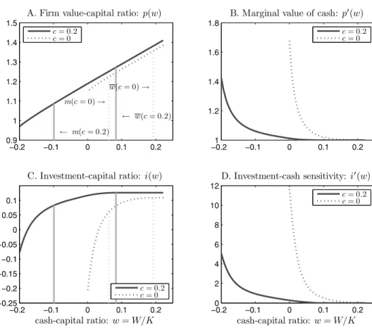
Next, we consider the setting in which the firm is allowed to issue equity. Fig-ure 3 displays the solutions for both the case with fixed financing costs (φ=1%) and the case without (φ=0). Observe that at the financing boundaryw=0, the firm’s value-capital ratiop(w) is strictly higher thanl, so that external equity financing is preferred to liquidation under this model parameterization. Com-pared with the liquidation case, we find that the endogenous payout boundary (marked by the solid vertical line on the right) isw=0.19 whenφ=1%, lower than the payout boundary for the case of liquidation (w=0.22). Not surpris-ingly, firms are more willing to pay out cash when they can raise new funds in the future. The firm’s optimalreturn cash-capital ratioism=0.06, marked by the vertical line on the left in Panel A. Without fixed costs (φ=0), the payout boundary drops further tow=0.14 and the firm’s return cash-capital ratio is zero, as the firm raises just enough funds to keepwabove zero.
Figure 3, Panel B, plots the marginal value of cash p(w), which is positive
and decreasing between zero and w, confirming thatp(w) is strictly concave in this case. Conditional on issuing equity and having paid the fixed financing cost, the firm optimally chooses the return cash-capital ratiomsuch that the marginal value of cash p(m) is equal to the marginal cost of financing 1+γ. To the left of the return cash-capital ratiom, the marginal value of cash p(w)
0 0.05 0.1 0.15 0.2 1 1.1 1.2 1.3 1.4 ← m(φ= 1%) w(φ= 1%)→ ← w(φ= 0)
A. Firm value-capital ratio: p(w)
φ= 1% φ= 0 0 0.05 0.1 0.15 0.2 1 1.2 1.4 1.6 1.8
B. Marginal value of cash: p(w)
φ= 1% φ= 0 0 0.05 0.1 0.15 0.2 0 0.1 0.2 cash-capital ratio: w=W/K C. Investment-capital ratio: i(w) φ= 1% φ= 0 0 0.05 0.1 0.15 0.2 0 2 4 6 8 10 12 cash-capital ratio: w=W/K D. Investment-cash sensitivity:i(w) φ= 1% φ= 0
Figure 3. Case II—optimal refinancing. This figure plots the solution for the case of refinancing.
lies above 1 +γ, reflecting the fact that the fixed cost component in raising equity increases the marginal value of cash. When the firm runs out of cash, the marginal value of cash is around 1.7, much higher than 1+γ =1.06. This result highlights the importance of fixed financing costs: even a moderate fixed cost can substantially raise the marginal value of cash in the low-cash region. As in the liquidation case, the investment-capital ratioi(w) is increasing inw and reaches the peak at the payout boundaryw, wherei(w)=11%. Higher fixed cost of financing increases the severity of financing constraints, therefore lead-ing to more underinvestment. This is particularly true in the region to the left of the return cash-capital ratiom, where the investment-capital ratioi(w) drops
rapidly. Asset sales go down quickly (i(w)>10) whenwmoves away from zero. This is because both asset sales and equity issuance are very costly. Remov-ing the fixed financRemov-ing costs greatly alleviates the underinvestment problem, where both the marginal value of cash and the investment-capital ratio become essentially flat except for very loww.
C. Average q, Marginal q, and Investment
We now turn to the model’s predictions for average and marginalq. We take the firm’senterprise value— the value of all the firm’s marketable claims minus cash, P(K,W)−W— as our measure of the value of the firm’s capital stock. Averageq, denoted byqa(w), is then the firm’s enterprise value divided by its capital stock:
qa(w)=
P(K,W)−W
K = p(w)−w. (22)
First, averageqincreases withw. This is because the marginal value of cash is never below one, so thatqa(w)=p(w)−1≥0. Second, averageqis concave provided thatp(w) is concave, in thatqa(w)=p (w).
In our model where external financing is costly, marginalq, denoted byqm(w), is given by qm(w)= dP(K,W)−W dK = p(w)−wp (w)=q a(w)− p(w)−1w, (23) whereqa(w)= p(w)−w(see equation (22)). An increase in capital stockK has two effects on the firm’s enterprise value. First, the larger the capital stock, the higher the enterprise value. This is the standard averageqchannel, where
qa(w) = p(w) −w. Second, increasing capital stock mechanically lowers the cash-capital ratiow=W/KforW>0, thus making the firm more constrained. The wedge between marginalqand averageq,−p(w)−1w, reflects this ef-fect of financing constraints on firm value. Withp(w)>1 andw >0, that wedge is negative, and marginal q is smaller than averageq. Third, both marginal
q and averageq increase with w for w >0, because p(w) is strictly concave. Finally, as a special case, under MM, p(w)= 1 and hence averageq equals marginalq.
Figure 4 plots the average and marginalqfor the liquidation case, the refi-nancing case with no fixed costs (φ =0), and the refinancing case with fixed costs (φ = 1%). The average and marginal q are below the first-best level,
qF B = 1.23, in all three cases, and they become lower as external financing becomes more costly.
D. Stationary Distributions of w, p(w), p(w), i(w), Average q, and Marginal q
We next investigate the stationary distributions for the key variables tied to optimal firm policies in the benchmark case with refinancing (φ=1%).18 We
first simulate the cash-capital ratio under the physical probability measure. To do so, we calibrate the Sharpe ratio of the market portfolioη=0.3, and assume that the correlation between the firm’s technology shocks and the market re-turn is ρ =0.8. Then, the mean of the productivity shock under the physical
18We conduct additional analysis of the effects of various parameters on the distributions of cash and investment in the Internet Appendix, which is available on theJournal of Financewebsite at http://www.afajof.org/supplements.asp.
0 0.05 0.1 0.15 0.2 0.25 0.9 0.95 1 1.05 1.1 1.15 1.2 cash-capital ratio:w=W/K A. Averageq case II (φ= 1%) case II (φ= 0) case I 0 0.05 0.1 0.15 0.2 0.25 0.9 0.95 1 1.05 1.1 1.15 1.2 cash-capital ratio:w=W/K B. Marginalq case II (φ= 1%) case II (φ= 0) case I
Figure 4. Averageqand marginalq. This figure plots the averageqand marginalqfrom the three special cases of the model. Case I is the liquidation case. Cases II and III are with external financing. The right end of each line corresponds to the respective payout boundary, beyond which bothqaandqmare flat.
probability is ˆμ=0.20. Figure 5 shows the distributions for the cash-capital ratiow, the value-capital ratiop(w), the marginal value of cash p(w), and the
investment-capital ratioi(w). Since p(w), p(w), andi(w) are all monotonic in this case, the densities for their stationary distributions are connected with that ofwthrough (the inverse of) their derivatives.
Strikingly, the cash holdings of a firm are relatively high most of the time, and hence the probability mass for i(w) is concentrated at the highest values in the relevant support of w, while p(w) concentrates mostly around unity. Thus, the firm’s optimal cash management policies appear to be effective at shielding itself most of the time from the states with the most severe financing constraints and underinvestment.
Table II reports the mean, median, standard deviation, skewness, and kurto-sis forw,i(w),p(w),qa(w),qm(w), andi(w). Not surprisingly, all these variables have skewness. The marginal value of cash and the investment-cash sensitivity are positively skewed, while the remaining variables have negative skewness. Interestingly, the kurtosis fori(w), p(w),qa(w), andi(w) is especially large, in contrast to their small standard deviations. Thefat tailfrom the distribution of cash holdings is dramatically magnified due to the highly nonlinear relation between these variables andw.
Empirical research on corporate cash inventory focuses mostly on firms’ av-erage holdings. As is apparent from Table II, avav-erage cash holdings provide an incomplete and even misleading picture of firms’ cash management, invest-ment, and valuation. The same is true for empirical estimates of the marginal value of cash and investment-cash sensitivity, which are generally interpreted as capturing how financially constrained a firm is. Even though the median
0 0.05 0.1 0.15 0.2 0 5 10 15 20 25 A. Cash-capital ratio: w 0 0.1 0 10 20 30 40 50 60 B. Investment-capital ratio: i(w) 1.1 1.2 1.3 1.4 0 5 10 15 20 25
C. Firm value-capital ratio: p(w)
1 1.2 1.4 1.6 0 5 10 15 20 25 30 35
D. Marginal value of cash: p(w)
Figure 5. Stationary distributions in the case of refinancing.This figure plots the prob-ability distribution functions (PDF) for the stationary distributions of cash holding, investment, firm value, and marginal value of cash for the case of refinancing withφ=1%.
and the mean of p(w) are close to one (and those ofi(w) close to zero), and even though both distributions have rather small standard deviations, the kurto-sis is huge for both, indicating that the firm could become severely financially constrained.
The impact of these low probability yet severe financing constraint states is evident. The mean and median ofqa(w) are 1.16, which is about 5% lower than qF B=1.23, the averageqfor a firm without external financing costs. Similarly, the mean and median ofi(w) is 0.104, which is about 31% lower thaniF B= 0.151, the investment-capital ratio for a firm without external financing costs. Therefore, simply looking at the first two moments for the marginal value of cash or investment-cash sensitivity provides a highly misleading description of firms’ financing constraints. Firms endogenously respond to their financ-ing constraints by adjustfinanc-ing their cash management and investment policies, which in turn reduces the time variation in investment, marginal value of cash, etc. However, the impact of financing constraints remains large on average.
Table II
Moments from the Stationary Distribution of the Refinancing Case
This table reports the population moments for the cash-capital ratio (w), the investment-capital ratio (i(w)), the marginal value of cash (p(w)), averageq(qa(w)), and marginalq(qm(w)) from the stationary distribution in the case with refinancing (φ=1%).
Cash-Capital Investment- Marginal Investment-Cash Ratio Capital Ratio Value of Cash Averageq Marginalq Sensitivity
w i(w) p(w) qa(w) qm(w) i(w) Mean 0.159 0.104 1.006 1.164 1.163 0.169 Median 0.169 0.108 1.001 1.164 1.164 0.064 Std. 0.034 0.013 0.018 0.001 0.001 0.376 Skewness −1.289 −6.866 9.333 −8.353 −3.853 8.468 Kurtosis 4.364 76.026 146.824 106.580 22.949 122.694
The analysis above highlights that, by providing a more complete picture of firms’ capital expenditures and cash holdings over the time series and in the cross-section, this model helps us better understand the empirical patterns of cash holdings. The model’s ability to match the empirical distributions can be further improved if we allow for changing investment and financing opportu-nity sets and firm heterogeneity.
IV. Dynamic Hedging
In addition to cash inventory management, the firm can also reduce its cash flow risk through financial hedging (e.g., using options or futures contracts). Consider, for example, the firm’s hedging policy using market index futures.19
Let Ftdenote the futures price on the market index at timet. Under the risk-adjusted probability, Ftevolves according to
dFt=σmFtdBt, (24) whereσmis the volatility of the aggregate market portfolio, andBtis a standard Brownian motion that is partially correlated with firm productivity shocks driven by the Brownian motionZt, with correlation coefficientρ.
Letψtdenote the hedge ratio, that is, the position in the market index futures (the notional amount) as a fraction of the firm’s total cashWt. Futures contracts often require that the investor hold cash in a margin account, which is costly. Letκtdenote the fraction of the firm’s total cashWtheld in the margin account (0 ≤ κt ≤ 1). In addition to the cash-carrying cost in the standard interest-bearing account, cash held in this margin account also incurs the additional flow cost per unit of cash. We assume that the firm’s futures position (in
19In this analysis, we only consider hedging of systematic risk by the firm. In practice, firms also hedge idiosyncratic risk by taking out insurance contracts. Our model can be extended to introduce insurance contracts, but this is beyond the scope of this article.
absolute value) cannot exceed a constant multipleπ of the amount of cashκt Wtin the margin account.20That is, we require
|ψtWt| ≤πκtWt. (25) As the firm can costlessly reallocate cash between the margin account and its regular interest-bearing account at any time, the firm will optimally hold the minimum amount of cash necessary in the margin account. That is, provided that > 0, optimality implies that the inequality (25) holds as an equality. When the firm takes a hedging position in the index future, its cash balance evolves as follows:
dWt=Kt(μdAt+σdZt)−(It+Gt)dt+dHt−dUt+(r−λ)Wtdt
−κtWtdt+ψtσmWtdBt.
(26)
Next, we investigate the special case in which there are no margin require-ments for hedging.
A. Optimal Hedging with No Frictions
With no margin requirement (π = ∞), the firm carries all its cash in the regular interest-bearing account and is not constrained in the size of the index futures positionψ. Since firm value P(K,W) is concave inW (i.e., PWW <0), the firm will completely eliminate its systematic risk exposure via dynamic hedging. The firm thus behaves in exactly the same way as the firm in our baseline model except that the firm is only subject to idiosyncratic risk with volatilityσ1−ρ2. It is easy to show that the optimal hedge ratioψis constant
in this case,
ψ∗(w)= − ρσ
wσm
. (27)
Thus, for a firm with sizeK, the total hedge position is|ψ W| = (ρ σ/σm) K, which linearly increases with firm sizeK.
B. Optimal Hedging with Margin Requirements
Next, we consider the important effects of margin requirements and hedg-ing costs. We show that financhedg-ing constraints fundamentally alter hedghedg-ing, investment/asset sales, and cash management. The firm’s HJB equation now becomes r P(K,W)= maxI,ψ,κ (I−δK)PK(K,W) +(r−λ)W+μK−I−G(I,K)−κWPW(K,W) +1 2 σ2K2+ψ2σ2 mW2+2ρσmσψW K PW W(K,W), (28)
subject to κ =min |ψ| π ,1 . (29)
Equation (29) indicates that there are two candidate solutions forκ(the fraction of cash in the margin account): one interior solution and one corner solution. If the firm has sufficient cash, so that its hedging choiceψ is not constrained by its cash holding, the firm setsκ= |ψ|/π. This choice ofκ minimizes the cost of the hedging position subject to meeting the margin requirement. Otherwise, when the firm is short of cash, it setsκ =1, thus putting all its cash in the margin account to take the maximum feasible hedging position:|ψ| =π.
The direction of hedging (long (ψ >0) or short (ψ <0)) is determined by the correlation between the firm’s business risk and futures return. Withρ >0, the firm will only consider taking a short position in the index futures as we have shown. Ifρ <0, the firm will only consider taking a long position. Without loss of generality, we focus on the case in whichρ >0, so thatψ <0.
We show that there are three endogenously determined regions for optimal hedging. First, consider the cash region with an interior solution forψ(where the fraction of cash allocated to the margin account is given byκ = −ψ/π <1). The first-order condition with respect toψis
πW PW+ σ2 mψW 2+ρσ mσW K PW W=0.
Using homogeneity, we may simplify the above equation and obtain ψ∗(w)= 1 w −ρσ σs − π p(w) p(w) 1 σ2 s . (30)
Consider next the low-cash region. The benefit of hedging is high in this region (p(w) is high whenw is small). The constraintκ ≤1 is then binding, henceψ∗(w)= −π for w≤ w−, where the endogenous cut off pointw− is the unique value satisfyingψ∗(w−)= −πin (30). We refer tow−as the maximum-hedging boundary.
Finally, whenwis sufficiently high, the firm chooses not to hedge, as the net benefit of hedging approaches zero while the cost of hedging remains bounded away from zero. More precisely, we have ψ∗(w) = 0 for w ≥ w+, where the endogenous cut off pointw+is the unique solution ofψ∗(w+)=0 using equation (30). We refer tow+as the zero-hedging boundary.
We now provide quantitative analysis for the impact of hedging on the firm’s decision rules and firm value. We choose the following parameter values:ρ = 0.8,σm=20%,π=5 (corresponding to 20% margin requirement), and=0.5%. The remaining parameters are those for the baseline case. These parameters and the key variables for the hedging case are also summarized in Table I.
Figure 6, Panel A, shows the hedging policy. We focus on the costly hedging case (depicted in solid lines). For sufficiently high cash balances (w > w+ = 0.11), the firm chooses not to hedge at all because the marginal benefit of