Statistical learning of high-dimensional directed acyclic graphical models

(1)

Statistical Learning of High-Dimensional Directed Acyclic

Graphical Models

A DISSERTATION

SUBMITTED TO THE FACULTY OF THE GRADUATE SCHOOL OF THE UNIVERSITY OF MINNESOTA

BY

Yiping Yuan

IN PARTIAL FULFILLMENT OF THE REQUIREMENTS FOR THE DEGREE OF

Doctor of Philosophy

Advised by Xiaotong Shen

(2)

c

Yiping Yuan 2015

(3)

Acknowledgements

I would like to express my endless gratitude to my advisor, Dr. Xiaotong Shen, for supporting me over the years, for teaching me the true spirit of research and for guiding me in my personal development. I have learned a great deal from working with Dr. Shen. His vision and encouragement helped me through hard times. My gratitude also goes to my other committee members, Dr. Wei Pan, Dr. Galin Jones and Dr. Charlie Geyer. It is very rewarding working with Dr. Pan, as his rigorous academic attitude and sharp questions are always inspiring. I want to thank Dr. Jones and Dr. Geyer for their advice and encouragement. In addition, I would like to thank Dr. Zizhuo Wang for bringing an outsider’s perspective and enriching the thesis with his expertise in optimization.

I would like to thank my friends at University of Minnesota with whom I have had the pleasure of working over the years. Thanks go to Yunzhang Zhu, Sen Yuan, Ben Sherwood, Yi Yang, Xin Zhang, Jie Ren as well as my other fellow students in the School of Statistics.

I also want to thank my parents for supporting me. Although I live across the pacific ocean over the years, I always feel their love and care. Finally, no words could express my special thanks to my beloved wife Jing. It has been a wonderful journey going through my five-year study with you.

(4)

Dedication

This dissertation is dedicated to my family, especially,

to my brilliant and outrageously loving and supportive wife, Jing Zhang;

to my always encouraging and supportive parents, Zhongwen Yuan and Li Cao, and parents-in law, Aibao and Chunhua Zhang.

(5)

Abstract

Directed acyclic graphs (DAGs) are widely used to describe directional relations among interacting units. Directional relations are estimated by reconstructing a DAG’s structure, which is a great challenge when the total ordering of a DAG is unknown. In such a situation, existing methods such as the neighborhood and search-and-score methods suffer greatly, as the overall estimation error accumulates super-exponentially in the number of nodes, especially when a local/sequential approach enumerates edge directions by testing or optimizing a criterion locally. In other words, a local method may break down even for moderately sized graphs. In this thesis, we propose a novel approach to simultaneously identify all estimable directed edges as well as model pa-rameters jointly. This approach uses constrained maximum likelihood with noncon-vex constraints reinforcing acyclicity. Computationally, we develop a novel reduction method that constructs a set of active constraints (cubic in the number of nodes) from the super-exponentially many constraints. This, coupled with an alternating direction method of multipliers and a difference convex method, permits efficient computation for large graph learning. Theoretically, we show that the proposed method consistently re-constructs identifiable directions of the true graph, under a degree of reconstructability assumption. This goes beyond the strong faithfulness assumption, commonly used in the literature. Moreover, the method recovers the optimal performance of the oracle es-timator in terms of parameter estimation. Numerically, the method compares favorably against its competitors.

Estimation of multiple directed graphs becomes challenging in the presence of in-homogeneous data, where directed acyclic graphs are used to represent causal relations among random variables. To infer causal relations among variables, we estimate multi-ple directed acyclic graphs given a known partial ordering in Gaussian graphical models. In particular, we propose a constrained maximum likelihood method with nonconvex constraints over elements and element-wise differences of adjacency matrices, for iden-tifying the sparseness structure as well as detecting structural changes over adjacency matrices of the graphs. Computationally, we develop an efficient algorithm based on

(6)

rithm for solving convex relaxation subproblems. Numerical results suggest that the proposed method performs well against its alternatives for simulated and real data.

For an observational study, correct reconstruction of a DAG’s structure from data is not always possible, because a DAG model is often not identifiable, which is the case for a Gaussian graphical model with unequal error variances. We study the problem of reconstruction of a DAG’s structure with the help of intervention observations. In particular, we construct a constrained likelihood to regularize intervention in addition to adjacency matrices to identify a DAG’s structure and remove redundant intervention variables. Importantly, we show that the constructed constrained likelihood yields cor-rect reconstruction of a DAG’s structure consistently provided that the candidate set of intervention variables includes the true informative ones. Computationally, we de-sign efficient algorithms for implementation. In simulations, we show that the proposed method enables to lead higher accuracy of reconstruction with the help of interventional observations.

(7)

List of Tables

2.1 Averaged false positive rate (FPR), false discover rate (FDR), Frobenius norm loss (FL), and Structural Hamming Distance (SHD), as well as their standard errors (in parenthesis), for four competing methods based on 100 simulation replications in Example 1. Here “Ours”, ”HC”, ”MMHC” and ”PC” denote ours, the HC, the MMHC and the PC methods. Note that N/A means that a method does not yield parameter estimation. . . 20 2.2 Averaged false positive rate (FPR), false discover rate (FDR), Frobenius norm

loss (FL), and Structural Hamming Distance (SHD), as well as their standard errors (in parenthesis), for four competing methods based on 100 simulation replications in Example 2. Here “Ours”, ”HC”, ”MMHC” and ”PC” denote ours, the HC, the MMHC and the PC methods. Note that N/A means that a method does not yield parameter estimation. Here∗represents no return value after 24 hour running time. . . 20 2.3 Frobenius norm loss (FL), and oracle rate (OR) for three competing methods

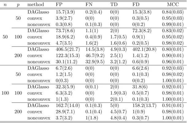
based on 100 simulation replications in Example 3. Here “Ours”, ”HC”, and ”MMHC” denote ours, the HC and the MMHC. . . 22 3.1 Estimated quantities and their corresponding estimated standard errors (in

parentheses) based on 100 simulation replications. For p = 50, there are 20 edges inG1 and 20 edges in G2 with no differences. Forp= 100, there are 88 edges inG1 and 86 edges inG2 with two differences. Forp= 200, there are 427 edges inG1 and 422 edges inG2with 5 differences. . . 37

(10)

Hamming Distance (SHD), as well as their standard errors (in parenthesis), for four competing methods based on 100 simulation replications. Here “Non-Int” and ”Int” denote the method in Chapter 2 applied to observational data only, and the proposed method applied to interventional data. . . 49

(11)

List of Figures

2.1 DAG representation of the true network in Section 5.2. . . 23 2.2 Reconstructed networks by various methods. True and false discoveries

are marked with green and red lines, where wrong directions are consid-ered to be false in this case. . . 24 2.3 Display of a consensus protein network consisting of eleven proteins. . . 25 2.4 Reconstructed networks using the proposed method and the other three

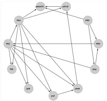
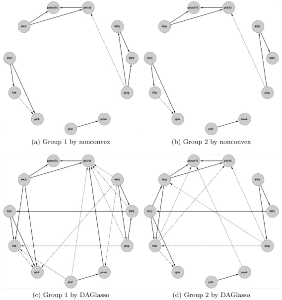
methods. Correct discoveries are marked in green, whereas false discover-ies are displayed in red. The network constructed by the PC is partially directed. . . 26 3.1 DAG representation for 11 proteins. . . 39 3.2 Analysis of cell signalling data: Correct edges are marked with solid

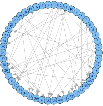
arrows, while false positives are indicated by long dashes. . . 40 4.1 The DAG used in the simulation study . . . 48

(12)

Chapter 1

Introduction

In this chapter, we briefly introduce related graph concepts and background knowledge, and then give an overview of the contribution of this thesis.

1.1 Definitions and Prelinimaries

Directed acyclic graphical models are widely used to represent and visualize directional relations, or parent-child relations, among interacting units, particularly in analyzing gene and social networks [1]. The graphical representation of the model is a directed acyclic graph (DAG), which, by definition, is a directed graph without directed cycles. Major building blocks of a DAG model are nodes, which represent random variables and edges, which encode conditional dependence relations of the enclosing vertices. A DAG G = (V, E) consists of a set of nodes V = 1, . . . , p and a set of directed edges E ⊆V ×V, that is, the edge set is a subset of ordered pairs of distinct nodes. In our setting, each node j represents a random variable Xj and an edge (i, j) ∈ E can be

denoted as i→j.

If there is a directed edge i→ j, node i is said to be a parent of nodej and nodej is called a child of node i. The set of parents of node iis denoted by pai. If there is a

directed path from nodeito nodej, then nodeiis called an ancestor ofjandjis called an descendant ofi. It can be shown that the absence of any directed cycles is equivalent to the existence of an ordering of nodes {v1, v2, . . . , vp} such that all edgesvi →vj have

i < j. Later in this thesis, we will see how the difficulty of the DAG learning differs

(13)

when the ordering of nodes is known and unknown.

The models encode graph-to-distribution correspondences through directed Markov properties. Let P denote the probabilistic distribution of (X1, X2, . . . , Xp).

Definition 1 ( Local Markov property) P is said to obey the local Markov property to the DAGGif every node is conditionally independent of its non-descendant, non-parent nodes given its parents.

∀i∈V :i⊥ {ndi\pai}|pai

where ndi are the non-descendants of i.

Definition 2 (Factorization property) We say thatP admits a factorization according to a DAG G if P(X1, . . . , Xp) = p Y j=1 P(Xj|paj).

In our case of a multivariate Gaussian distribution, both properties in Definition 1 and Definition 2 are equivalent. For more details see [2].

In this thesis, we focus on Gaussian DAGs. We assume throughout the thesis that

X = (X1, X2, . . . , Xp) follows multivariate normal distribution. The Gaussian

assump-tion implies that E(Xi|pai) is linear in pai. Statistically, the model can be written as

Xj =

X

k∈paj

AjkXk+Zj, Zj ∼N(0, σj2); j= 1, . . . , p,

whereZj represents random error andAis the parameter matrix of interest. This thesis

is devoted to infer the model from data observed for X.

1.2 Overview of the contribution in this thesis

In this thesis, we develop a simultaneous reconstruction approach to estimate the con-figuration of a DAG and model parameters jointly, especially for the high-dimensional cases. This approach overcomes the difficulties of local and sequential approaches in the literature. Specifically, we propose a constrained likelihood for reconstructing a DAG without a known ordering in Chapter 2. Our novel treatment to this seemingly impossible problem is utilizing a property of doubly stochastic matrices to derive an

(14)

equivalent form involving only p3−p2 active constraints, c.f., Theorem 1. This, com-bined with a constrained alternating direction method of multipliers [3] and difference convex programming, makes it possible to solve this problem, thus leading to efficient computation involving a complexity of orderO(p3). Theoretically, we develop a theory to quantify what the proposed method can accomplish, where the focus is equal error variance for identifiable DAG models [4]. We show that it consistently reconstructs the true directed acyclic graph under a degree of reconstructability assumption (2.19). This assumption, similar to the “beta-min” condition [5], requires that the minimum separa-tion between the target and candidate models exceeds a certain threshold. Note that the corresponding probabilistic distribution may not be identifiable in general in the pres-ence of equivalpres-ence classes of DAGs [6]. With regard to estimating model parameters, it recovers the optimal performance of the oracle estimator.

We next study multiple DAG learning when data are inhomogeneous and proposed a maximum likelihood method to jointly estimate multiple DAGs with a known order-ing. To achieve our goal of learning graphical structures, we construct two nonconvex constraints based on the truncatedL1-function (TLP, [7]), as a computational surrogate

of the L0-function, with one constraint imposing sparseness and the other encouraging

a common structure. Computationally, with difference convex programming and aug-mented Lagrange multipliers, nonconvex minimization is solved through a sequence of convex subproblems iteratively. For each subproblem, we develop a fast algorithm to treat a constrainedL1-problem, which we call pairwise coordinate descent algorithm.

In Chapter 4, we study how incorporating interventional data could make a difference in identifying causal directions. For an observational study, a DAG model is often not identifiable. In such cases, correct reconstruction of a DAG’s structure from data is impossible. In Chapter 4, we study the problem of reconstruction of a DAG’s structure with the help of intervention observations. In particular, we construct a constrained likelihood to regularize intervention in addition to adjacency matrices to identify a DAG’s structure and remove redundant intervention variables. Importantly, we show that the constructed constrained likelihood yields correct reconstruction of a DAG’s structure consistently, provided that the candidate set of intervention variables includes the true informative ones.

(15)

(16)

Chapter 2

Constrained likelihood for

reconstructing a directed acyclic

Gaussian graph

In this chapter, we introduce the constrained likelihood approach for reconstructing a directed acyclic Gaussian graph. Section 2.1 covers existing methods. Section 2.2 intro-duces the proposed method. Section 2.3 is devoted to the computational development of the proposed method. Section 2.4 presents theoretical results concerning structure pursuit and parameter estimation. Section 2.5 performs simulation studies to compare with several competing methods, and analyzes a protein network. Section 2.6 discusses the methodology. Finally, the Appendix contains technical proofs.

2.1 Background of DAG Learning

In the literature, most existing methods are designed for a low-dimensional situation, in which the size of a graph is relatively small compared with the sample size. Major approaches emerge in two categories. The first uses multiple local conditional indepen-dence tests sequentially [8, 9, 10] to enumerate possible directions through the local Markov property. Such methods usually have a worst case exponential complexity in

(17)

the number of nodes, including the most popular “PC” algorithm. [11] proposed a high-dimensional modification to the original “PC”. This modified “PC” has a complexity of order O(pq) withp nodes, whereq is the maximal neighborhood size. However, this complexity becomes super-exponential when q is large q = O(p) even if the graph is sparse; see Example 2 in Section 4. The second, referred to as “search-and-score”, op-timizes a goodness-of-fit measure for possible directions in a neighborhood of interest [12, 13, 14]. Computationally, search-and-score methods suffer greatly from the curse of dimensionality due to O(p!2p2) candidate DAGs ofp labeled nodes [15]. Moreover, due to their sequential nature, they tend to yield unstable and deteriorating performance for a large graph. The major difficulty comes from acyclicity, as pointed out in [16, 17, 18] and recently [19, 20]. As a result, the recent development of DAG models lags be-hind that of undirected graphs [21] in the high-dimensional situation. Nevertheless, we would like to mention two recent developments on special situations. [22] proposed a L1-penalization method for learning the DAG model with a known topological ordering

of the nodes. [23] used aL1-penalization method for interventional data.

Nonconvex optimization for exact learning of a DAG’s structure, for instance, [24], focuses on identifying an exact global optimizer for this NP-hard problem. Certain approximations are involved with a worst-case suboptimality bound for an anytime solution, which is an approximate solution when the algorithm can be interrupted at any time before it takes too long. As a result, it is rather difficult, if not impossible, to treat even a moderate graph with more than one hundred nodes. Recently, mixed integer linear programming (MILP) has been used together with certain branch-and-bounds [25, 26, 27, 28].When the maximal number of parent nodes is restricted to one or two, such a method may handle a larger graph than the previous exact methods. Again, such a restriction limits the scope of application. In this article, based on a difference convex algorithm, we seek a good optimizer that is shown to be local for fast convergence, although such an optimizer may be sometimes global. This is in contrast to the counterpart of our DC algorithm, such as Breiman and Cutler’s outer approximation method [29] that guarantees globality of a solution at an expense of slow convergence. Importantly, as showed in Table 3, our DC algorithm may have a good chance to identify a global optimizer. This aspect of a DC algorithm has been previously noted in [30] for a linearly constrained indefinite quadratic problem.

(18)

In addition to the computational challenges in the high-dimensional situation, theo-retical challenges remain. First, it is challenging statistically in that the error of correct reconstruction of a DAG may grow super-exponentially in p. Roughly, this error is no less than min(1,exp(plogp−b(ε)n)) in view of Bahadur’s lower bound for the error of each test [31], where b(ε) is a constant describing the least favorable situation defined by the Kullback-Leibler information. In other words, any local and sequential method, particularly the PC algorithm and its variants, may break down, which occurs roughly when plogp significantly exceeds n. Second, there is paucity of theory to guide prac-tice for reconstruction of a DAG. One relevant theory is on consistent reconstruction of a DAG’s structure for the PC-algorithm [11], which relies on one key assumption, called “strong faithfulness” [8, 32]. Unfortunately, this assumption is rather restric-tive, because it induces a small set of distributions as pointed out in [33]. Thus one open problem is whether any computationally feasible method can lead to consistent reconstruction of a DAG beyond the “strong faithfulness”.

In this chapter, we develop a simultaneous reconstruction approach to estimate the configuration of a DAG and model parameters jointly. This approach overcomes the aforementioned difficulties of local and sequential approaches. Specifically, we propose a constrained likelihood with a set of O(pp) nonconvex constraints, to quantify the pa-rameter space for DAG’s. This reinforces the local Markov property that is crucial to discovering directional relations. Our novel treatment to this seemingly impossible problem is utilizing a property of doubly stochastic matrices to derive an equivalent form involving only p3−p2 active constraints, c.f., Theorem 1. This, combined with a constrained alternating direction method of multipliers [3] and difference convex pro-gramming, makes it possible to solve this problem, thus leading to efficient computation involving a complexity of order O(p3). Theoretically, we develop a theory to quantify what the proposed method can accomplish, where the focus is equal error variance for identifiable DAG models [4]. We show that it consistently reconstructs the true directed acyclic graph under a degree of reconstructability assumption (2.19). This assumption, similar to the “beta-min” condition [5], requires that the minimum separation between the target and candidate models exceeds a certain threshold. Note that the corre-sponding probabilistic distribution may not be identifiable in general in the presence of equivalence classes of DAGs [6]. With regard to estimating model parameters, it

(19)

recovers the optimal performance of the oracle estimator.

2.2 Statistical methods

A DAG model encodes a joint probability distribution of a random vector (X1, . . . , Xp),

whose nodes and directed edges represent X1, . . . , Xp and parent-child dependence

re-lations between any two variables. The parents of Xj, denoted as paj, is the set of

variables with a direction towards Xj in the graph. The model factorizes the joint

dis-tribution of (X1, . . . , Xp),P(X1, . . . , Xp), into a product of conditional distributions of

each variable given its parents, that is,Qp

j=1P(Xj|paj), where paj denotes a parent set

of Xj and is defined to be empty if Xj has no parents. This factorization property is

equivalent to the local Markov property [34] in the DAG case, and is closely related to antedependence [35], which has been widely used in time series and longitudinal data analysis.

A DAG over nodes{1,· · ·, p}is uniquely defined by anp×padjacency matrixAin which a nonzerojk-th elementAjkofAcorresponds to a directed edge from parent node

k to child notej with its value Ajk indicating the strength of the relation. The DAG

does not contain a dicycle, where existence of a dicycle for a directed graph destroys the local Markov property of a DAG.

2.2.1 DAG parameter space

Most statistical methods focus on construction by optimizing a suitable cost function, since the parameter space is usually a simple convex space, for example, the Rp space for regression and the positive semidefinite cone Sp+ = {A ∈ Rp×p|A = AT,A

0} for Gaussian undirected graphical models [36]. In contrast, the parameter space of the Gaussian DAG models is defined as {A ∈ _Rp×p _: _G₍_A_{) is a DAG}_}_{, which is}

nonconvex as a result of nonconvex constraints reinforcing acyclicity of a graph [5]. Yet, characterization of the parameter space remains an open problem. In what is to follow, we develop a method to deal with such an irregular parameter space.

To introduce acyclicity constraints, denote a directed cycle (dicycle) by (j1, . . . , jL),

a sequence of indices of nodes, where L is the length of the dicycle, and j1 is required

(20)

example, a dicycle 1 ← 2← 3 ←1 is denoted as (1,2,3). A DAG, by definition, does not contain a dicycle. This implies that the number of directed edges is smaller than the number of involved nodes in every possible dicycle [37]. Let I(·) be the indicator function. To prevent a dicycle, say (1,2,3), from occurring, we introduce a constraint I(A1,2 6= 0) +I(A2,3 6= 0) +I(A3,1 6= 0) ≤ 2 to require that the number of directed

edges be smaller than the number of involved nodes in every possible cycles. Note that this requirement is necessary and sufficient. On this basis, we introduce constraints on entries ofA to reinforce acyclicity of any order:

X

j1=jL+1:1≤k≤L

I(Ajkjk+1 6= 0)≤L−1; any dicycle (j1, . . . , jL), L= 2, . . . , p, (2.1)

where order L is the number of nodes in a possible dicycle. It is important to remark that any orders of dicycle are permissible if the corresponding constraints are reinforced in (2.1). For instance, any dicycle of order exceeding 2 are allowed if L= 3,· · ·, p are removed from (2.1). Moreover, L = 1 corresponds to self-loops, which is characterized by nonzero diagonals. Critically, the total number of constraints in (2.1) is p₂+ p₃2! +

· · ·+ p_p

(p−1)! = O(pp), which is super-exponential in p. The parameter space of Gaussian DAG models is thus defined by the O(pp) DAG constraints over A.

Next we present our main result on constraint reduction to reduce the O(pp) con-straints in (2.1) to p3 −p2 constraints in (2.2). This result is based on duality and properties of permutation matrices, and can be used with any optimizing function.

Theorem 2.2.1 (Construction of a set of active constraints) The adjacency matrix A

satisfies the acyclicity constraints in (2.1)if and only if there exists ap×pdual variable matrix λ= (λjk)p×p∈Rp×p such that the following constraints are satisfied by A.

λik+I(j6=k)−λjk ≥I(Aij 6= 0);i, j, k = 1, . . . , p, i6=j. (2.2)

In (2.2), there arep3−p2 constraints over (A,λ) through additional slack variables. This allows us to not only reduce super-exponentially many constraints overAtop3₋_p2

active constraints over (A,λ) but also achieve simplicity in that each constraint involves only one parameter in Aand is linear in λjk and I(Aij 6= 0).

(21)

2.2.2 Constrained maximum likelihood

Statistically, we embed directional effects induced by directed edges through A into a structural equation model. A structural model can be written as:

Xj =fj(paj, Zj), j = 1, . . . , p, (2.3)

where Zj is latent error representing unexplained variation in each node, and the local

Markov property is defined through parents and latent variables in (2.3).

Now consider a Gaussian structural equation model in which each fj(·,·) in (2.3)

becomes linear in (pa_j, Zj), and eachZj follows normal distributionN(0, σ2):

Xj =

X

k6=j

AjkXk+Zj, Zj ∼N(0, σ2); j= 1, . . . , p, (2.4)

whereAjk is 0 whenk6∈paj. In (2.4), our objective is to estimate parametersAsubject

to the requirement thatAdefines a DAG. This enables us to determine zero-entries ofA

to identify all parent-child relations as well as to estimate the strengths of the relations defined by nonzero-entries of A simultaneously. Note that individual means can be incorporated by adding intercepts into (2.4) but it is less relevant to reconstruction. For simplicity, we therefore set the means to be zero in what is to follow. Note that in (2.4) an equal variance for Zj’s leads to identifiable DAGs [4]. A more general case

with different error variances will be discussed in Section 4.

Given n×p data matrix X sampled from (2.4), with its ij-th entry xij being the

i-th observation on the j-th node, the negative loglikelihood, after dropping a constant term, is l(A) = 1 2 p X j=1 n X i=1 xij − X k6=j xikAjk 2 , (2.5) which is convex inA.

For estimation ofA, we impose a constraint to regularize sparsity ofA, in addition to constraints defined in (2.1). The first constraint controls nonzero entries of A

X

j6=k

I(Ajk 6= 0)≤K,

where I(·) is the indicator function, and K is an integer-valued tuning parameter con-trolling the degree of sparsity.

(22)

The DAG learning problem can be formulated as follows: minAl(A) (2.6) subject to P j6=kI(Ajk 6= 0)≤K, P j1=jL+1:1≤k≤LI(Ajkjk+1 6= 0)≤L−1; any dicycle (j1, . . . , jL), L= 2, . . . , p.

Using the result from Theorem 1, (2.6) is equivalent to

min(A,λ)l(A) (2.7)

subject to P

j6=kI(Ajk 6= 0)≤K, (2.8)

λik+I(j6=k)−λjk ≥I(Aij 6= 0);i, j, k = 1, . . . , p, j6=i. (2.9)

Next we approximate the indicator functions to circumvent the difficulty of non-discontinuity in minimization. Specifically, in (4.4) and (2.9), we substitute the indicator functions by its computational surrogateJτ(·) where Jτ(x) = min(|x_τ|,1) is the truncated

L1-function (TLP) [7], which approximates the indicator function asτ →0+. This yields

that

min(A,λ)l(A) (2.10)

subject to P

1≤j6=k≤pJτ(Ajk)≤K, (2.11)

λik+I(j6=k)−λjk ≥Jτ(Aij);i, j, k= 1, . . . , p, j6=i. (2.12)

Minimization (2.10) subject to (2.11) and (2.12) involves p3 −p2 + 1 nonconvex constraints in (2.12). Yet, compared to the original formulation with indicator func-tions, Jτ(·) is piecewise linear and can be decomposed into the difference of two convex

functions. Next we solve this constrained minimization through difference convex pro-gramming and the alternating direction method of multipliers (ADMM).

2.3 Computation

This section develops our computational strategy to solve (2.10). Our strategy proceeds in two steps. First, we relax (2.11) and (2.12) using a sequence of approximations involving convex constraints, where each approximation is refined iteratively. Then we solve each convex subproblem with p3 −p2 + 1 linear constraints by employing a

(23)

constrained alternating direction method of multipliers. The underlying process iterates until convergence.

For convex relaxation of constraints (2.11) and (2.12), we employ the difference convex (DC) programming. In particular, we decompose Jτ into a difference of two

convex functions: Jτ(z) = S1(z)−S2(z) = |z_τ| −max(|z_τ| −1,0). On this ground, we

construct a sequence of convex approximating sets iteratively by replacing S2 in the

decomposition at iteration m by its affine majorization at iterationm−1. Specifically, we solve min (A,λ)l(A) subject to X i6=j |Aij|w (m−1) ij ≤Z (m−1)_, τ λik+τ I(j6=k)−τ λjk ≥ |Aij|w(m −1) ij +τ(1−w (m−1) ij );i, j, k = 1, . . . , p, j6=(2.13)i,

where w_ij(m−1) = I(|Aˆ_ij(m−1)| ≤ τ), and ˆA(m−1) _{is the solution at iteration} _m₋_{1; 1} _≤ i, j ≤p. Z(m−1)=τ K−P i6=j(1−w (m−1) ij )

. At iterationm, we solve a minimization problem with p3−p2+ 1 linear constraints.

To solve (2.13), we consider its equivalent form for efficient computation: min(A,λ)l(A) +µ P i6=j|Aij|w (m−1) ij subject to τ λik+τ I(j6=k)−τ λjk ≥ |Aij|w(m −1) ij +τ(1−w (m−1) ij );i, j, k= 1, . . . , p, j6=(2.14)i,

whereµis a nonnegative regularizer corresponding toZ(m−1)_{in (2.13). Their}

correspon-dence is as follows: Given a solution of (2.14) ( ˜A(µ),λ˜(µ), µ), A˜(µ), ˜λ(µ), Z(m−1)is a global minimizer of (2.13), whereZ(m−1)=P

i6=j|A˜ij(µ)|w(m

−1)

ij , and vice versa.

There-fore,Z(m−1)can be obtained through bisection ofµsuch thatZ(m−1)=P

i6=j|A˜ij(µ)|w

(m−1)

ij .

Based on our limited numerical experience, ADMM may significantly expedite con-vergence, although (2.14) may be solved by a quadratic programming solver. To pro-ceed, let ξ = {ξijk}p×p×p be a slack variable tensor, converting inequality to equality

constraints. Then (2.14) becomes

min₍_A_,_λ₎l(A) +µP i6=j|Aij|w(m −1) ij subject to τ λik+τ I(j6=k)−τ λjk− |Aij|w(m −1) ij −τ(1−w (m−1) ij )−ξijk = 0; i, j, k = 1, . . . , p, j6=i, ξijk ≥0. (2.15)

(24)

Next we introduce Bp×p to separate the differentiable from non-differentiable parts

involvingL1-norm. Then the problem can be written in the form as

min(A,λ)l(A) +µ P i6=j|Bij|w(m −1) ij subject to τ λik+τ I(j6=k)−τ λjk− |Bij|w(m −1) ij −τ(1−w (m−1) ij )−ξijk = 0; i, j, k = 1, . . . , p, j6=i, ξijk≥0,A−B=0. (2.16)

Following [38], we obtain an augmented Lagrangian by introducing the scaled dual variable tensor y={yijk}p×p×p and the scale dual variable matrix U ={yij}p×p:

Lρ(A,B,λ,ξ,y,U) =l(A) +µ(Pi6=j|Bij|w(m −1) ij ) + ρ 2kA−B+Uk2F (2.17) +P k P i6=j ρ 2 |Bij|w(m −1) ij +τ(1−w (m−1) ij ) +ξijk−λik−τ I(j6=k) +λjk +yijk 2 . Iteratively, we solve (2.17) over six blocks (A,B,λ,ξ,y,U). At iteration step s+ 1,

A(s+1) = argmin_ALρ(A,B(s),φ(s),λ(s),ξ(s),y(s),U(s)), B(s+1) = argmin_BLρ(A(s+1),B,φ(s),λ(s),ξ(s),y(s),U(s)), λ(s+1) = argmin_λLρ(A(s+1),B(s+1),φ(s),λ,ξ(s),y(s),U(s)), ξ(s+1) = argmin{ξijk≥0}Lρ(A (s+1)_,_B(s+1)_,_φ(s)_,_λ(s+1)_,_ξ_,_y(s)_,_U(s)₎_, y_ijk(s+1) = y_ijk(s)+|B_ij(s+1)|w_ij(m−1)+τ(1−w(_ijm−1)) + +ξ(_ijks+1)−τ λ(_iks+1)−τ I(j6=k) +τ λ(_jks+1), U(s+1) = U(s)+ A(s+1)−B(s+1),

where analytic formulas are given in the Appendix.

Overall, our computational algorithm is summarized as follows.

Algorithm 1:

Step 1. (Initialization) Supply a good initial estimate ˆA(0), such as ˆA(0)=0.

Step 2. (Iteration) At iterationm, compute ˆA(m)by solving (2.13) through our ADMM.

Step 3. (Termination) Terminate when l( Â(m−1))−l( Â(m)) ≤ ε, where ε is the the precision tolerance. Then the estimate Â = Â(m∗), wherem∗ is the smallest index at the termination criterion.

Proposition 1 (Computational property of Algorithm 1) Algorithm 1 converges, which yields a DAG when τ is sufficiently small such that |Aij| ≥ τ for all edge (i, j) ∈ E,

(25)

and is a local minimizer of (2.10)subject to (2.11)and (2.12)in that it satisfies a local optimality condition: For some multipliers ν≥0 and{ζijk≥0}i,j,k=1,...,p,j6=i,

∂l(A) ∂Aij +ν τsij + P 1≤k≤pζijk τ sij = 0; i, j= 1,· · ·, p, (2.18)

where sij is subdifferential defined as sij = sign(Aij) if 0 < |Aij| < τ; Aij ∈ [−1,1]

if Aij = 0; sij = 0 if |Aij| > τ; sij = ∅ if |Aij| = τ, is the regular subdifferential of

Jτ(|Aij|)atAij, and ∅is the empty set. The reader may consult [39] for subdifferentials

of continuous but nondifferentiable functions.

The computation complexity for our algorithm in one iteration over six blocks in (2.18) is roughly O(p3+np2) given p2 parameters in A. With regard to convergence, it is usually the case that ADMM converges with modest accuracy within a few tens of iterations, although ADMM can be slow to converge with high accuracy [38]. This is in contrast to fast convergence of the DC part, which has finite termination property [40]. Based on our limited experience, our DC step converged within ten iterations for our examples.

2.4 Theory

This section develops a theory for the constrained maximum likelihood (MLE) with respect to reconstruction of a DAG’s structure. We will show that the proposed method recovers the true DAG’s structure under the assumption (2.19). We will proceed under the equal variance assumption, which implies that the distributions from different DAG models are identifiable [4].

To introduce notations, let B= (G,θ) be a parametrized DAG, where θ = (A, σ), G = G(A) is a DAG induced by parameters. Let E = E(A) = {(i, j) : Ai,j 6= 0}

be the set of nonzero elements in A, which is equivalent to the edge set of the graph. Let F₀ = {θ = (A, σ) : cmin(Ω) ≥ M1 > 0; sup1≤j≤p|Ωjj| ≤ M2} be the parameter

space containing (A0, σ0), where M1, M2 > 0 are two constants, Ω = (I −A)T(I − A)/σ2 and cmin(Ω) is the smallest eigenvalue of Ω. Note that the assumption that

infA∈F0cmin(Ω)≥M1>0 and sup1≤j≤p|Ωjj| ≤M2suffices to ensure that the likelihood

(26)

In what is to follow, we will derive a finite-sample probability error bound for recon-structing the true DAG by the proposed method. As a result, the proposed method not only reconstructs the true DAG when identifiable, but also recovers the optimal param-eter estimation of the oracle estimator ( ˆAOR,σˆOR), defined as the maximum likelihood estimator assuming that the true edge setE0 (or the nonzero set ofA0 equivalently) is known as a priori.

Assumption A: For some positive constants M1 and M2, infΩcmin(Ω)≥M1 >0

and sup₁≤k≤p|Ωkk| ≤M2, wherecmin(Ω) is the smallest eigenvalue ofΩand Ωkkis the

kth diagonal of Ω.

Assumption A is a regularity condition on boundedness of entries ofΩ. Assumption A implies that σ2 ≥M₂−1 since Ωjj = _σ12 +

P

k6=j σ12A2_jk for a DAG matrix. Moreover,

from (2.4), σ2 ≤Var(Xj) = Σjj =eTjΣej ≤1/cmin(Ω)≤1/M1, whereek is a standard

basis vector with kth element being 1. Therefore,σ2 is bounded above and below. Next define the degree of reconstructability for DAGs, to be

Cmin(Ω0) = inf {ΩE=(I−AE)T(I−AE)/σ2:AE6=A0,|E|≤|E0|,AE satisfies(2.1)} −log(1−h2(ΩE,Ω0)) max(|E0_\_E_|_,₁₎ , where h2(Ω,Ω0) = 1− r (det(Ω)det(Ω0₎₎1/2

det(Ω+₂Ω0) is the Hellinger-distance between Ωand Ω 0

under (2.4). Note that under regularity conditions, a Taylor’s expansion of logdet(Ω) atA0 yields that −2 log 1−h2(ΩE,Ω0) =−1 2 log det ΩE

+ log det Ω0+ log det

Ω_E+Ω0 2 ≥ 1 8( ~ AE−A~0)TH(A~E−A~0)≥c∗|E0\E|cmin(H)γmin2 ,

for some constant c∗ > 0, where A~ is a p2 vector representation of A, where γmin ≡ γmin(A0) = min{|A0_jk|:A0_jk 6= 0, j 6=k} is the minimal of nonzero entries of A0 whose ijth element isAij, andH =

_∂2₍₋_{log det((}_I₋_A₎T₍_I₋_A₎_/σ2₎₎

∂2_A

|_A₌_A0 is thep2×p2 Hessian

matrix of−logdet(Ω). ThenCmin(Ω0)≥c∗γ_min2 cmin(H), see [41] for such an expansion.

In view of the foregoing connection, the degree of reconstructability measures the overall degree of difficulty for reconstruction, which is closely related to two terms. Whereas γ_min2 (A0) reflects the signal strength in terms of the minimal nonzero size

(27)

of Ω0, cmin(H) can be thought of as the local curvature of log-determinant of Ω0,

measuring dependency among entries of Ω0. In a sense, both the terms are critical for reconstruction.

Our key assumption requires the degree of reconstructability exceeds a certain threshold that is proportional ton−1max(logp,|E0|).

Assumption B:(Degree of reconstructability). Assume that

Cmin(Ω0)≥4c−21n

−1_max(log_p,_|_E0_|₎_, _(2.19)

for some positive constant c2 >0, sayc2= ₂₇2 ₉₆₃1 .

For reconstruction, we show that the proposed method enables us to consistently reconstruct the true DAG, yielding the optimal estimation, provided that the degree of reconstructability exceeds a certain level n−1logp.

The next theorem says that the oracle estimator ˆΩOR= (I−AˆOR)T(I−AˆOR)/(ˆσOR)2 is constructed by a global minimizer ˆθL0 _{= ( ˆ}_AL0_,_ˆ_σL0_{) of (2.7) subject to (4.4) and (2.9).}

As n, p,|E0| → ∞, the reconstructed DAG ˆGL0 _{is consistent for the true DAG} _G0_;

moreover, the optimal performance Eh2( ˆΩOR,Ω0) as measured by the Hellinger-risk is recovered byEh2_{( ˆ}_ΩL0_,_Ω0_).

Theorem 2.4.1 (L0-method) Under Assumption A, if K =|E0|in (4.4), then there

exists a constant c2>0, say c2= ₂₇2 ₉₆₃1 , such that for any (n, p,|E0|), PGˆL0 ₆₌_G0 ≤P( ˆΩL0 ₆_{= ˆ}_ΩOR₎_≤_exp ₋_c 2nCmin(Ω0) + 2 log (p(p+ 1) + 1) + 1 . (2.20) Under Assumption B, PGˆL0 ₆₌_G0 →0, and Eh2( ˆθL0,θ0) Eh2_{( ˆ}_ΩOR_,_Ω0₎ →1, asn, p,|E 0_{| → ∞.}

A similar result is established by the proposed estimator–the minimizer ˆθT = ( ˆAT,DˆT) of (2.10) subject to (2.11) and (2.12) given additional Assumption C.

Assumption C:For some positive constants d1, d2, d3,

h2(Ω,Ω0)≥d1h2(Ωτ,Ω0)−d3pτd2, (2.21)

whereΩτ = (I−Aτ)T((I−Aτ)/σ2, and theijth element ofAτ is defined asAijI(|Aij| ≥

τ).

(28)

τ ≤Cmin(Ω0)M1/4p, then there exists a constantc2 >0, sayc2 = ₂₇4 ₁₉₂₆1 , such that for any (n,|E0|, p), P ˆ GT 6=G0

≤P( ˆΩT 6= ˆΩOR)≤exp −c2nCmin(Ω0) + 2 log (p(p−1) + 1) + 1

.

Under Assumption B, PGˆT 6=G0→0, Eh2(ΩˆT,Ω0)

Eh2₍ΩˆOR_,_Ω0₎ →1, asn, p,|E

0_{| → ∞.}

The graphical structure is recovered by ˆθL0 _{and its computational surrogate ˆ}_θT _as

well as the optimal performance of the oracle estimator.

Next we comment on technical conditions in Assumptions A and B. Assumption A is a regularity condition for Ω. Assumption B may be viewed as an alternative to the strong faithfulness, which is defined as follows. Givenκ∈(0,1), a multivariate Gaussian distribution is said to be κ-strong-faithful to a DAG G= (V, E) if for any i, j∈V and any S ⊂V\{i, j}:

min{|corr(Xi, Xj|XS)|:j notd-separated from i,1≤i, j≤p}> κ, (2.22)

whereκ is of orderps0logp/n, and s0 is some kind of sparsity measure. Note that for

a pair of (i, j), the number of possible setS isPp−2

j=1

p−2

j

= 2p−2. If there is a directed edge betweeniand j, thenj is notd-separated fromigiven any of theseS. Therefore, for this (i, j) pair alone, there are actually exponentially many conditions to fulfill. In other words, theκ-strong-faithfulness condition excludes exponentially many sets of dis-tributions with nonzero Lebesgue measures. Even though these sets overlap, empirical studies in [33] show that the proportion ofκ-unfaithful distributions could approach 1 in some situations. This suggests (2.22) is very restrictive. As argued in the introduction, a PC algorithm may not work when plogp >> n in view of Bahadur’s lower bound, suggesting that (2.22) may break down in this case. It seems that Assumption B is not subject to this restriction, although a direct connection between Assumption B and (2.22) remains unclear.

As a technical remark, we note that the proposed methodology is applicable to the situation of nonequal error variances in (2.4), although the focus of this chapter is the identifiable situation assuming equal error variances. This error variance assumption seems sensible for consistent DAG reconstruction and natural for applications with variables from a similar domain, which has been commonly used in time series models.

(29)

When the error variances are not equal in (2.4), our method continue to work with a minor modification of the likelihood function. In such a situation, DAG models are no longer identifiable, and the equivalence classes are estimated as opposed to DAGs; see [6] for a detailed discussion.

2.5 Numerical Results

This section examines operating characteristics of the proposed method, and compares it against its strong competitors via simulations in terms of estimation accuracy of directed edges and parameter estimation. Specifically, the proposed method is contrasted with three top performers. They are a test-based PC algorithm [8], a score-and-search Hill Climbing method [42] and a hybrid version Max-Min Hill Climbing (MMHC, [43]), denoted as PC, HC and MMHC, respectively. For our method, we code in C and embed into an R-package. For PC, we use the R-package pcalg. For HC and MMHC, we use the R-package bnlearn. In what follows, two simulated examples are considered in Section 5.1, in addition to one real data example in Section 5.2.

For accuracy of estimating directed edges of a graph, we consider the false positive rate (FPR) and the false discovery rate (FDR), defined as FPR = FP/(FP + TN) and FDR = FP/(TP + FP), where TP, FP, TN and FN are true positive, false positive, true negative and false negative numbers of edge estimation, respectively.

For overall accuracy of estimating the DAG structure, we employ a commonly used measure–Structural Hamming Distance (SHD). The SHD between two DAGs is the required number of edge insertions, deletions or flips to transform one graph to another graph, c.f., [43]. A smaller SHD indicates closeness of two graphs. To compute the SHD, one may consider the R-package pcalg.

For accuracy of parameter estimation of the adjacency matrixA, we use the Frobe-nius norm loss (FL) to measure discrepancy between an estimator ˆAand the truth A0:

F L( ˆA,A0) = v u u t p X i=1 p X j=1 (Aij−A0ij)2 (2.23)

(30)

For the proposed method, two tuning parameters (τ, K) are estimated using a tuning set. As suggested in [7], τ needs to be sufficiently small for a good approximation. In our case, τ is set to be{0.1,0.01,0.001},K is an integer valued from 1 to 150, an upper bound of the maximum number of edges in the graph, controlling the degree of sparsity of a graph. Then we minimize the predicted log-likelihood in (2.5) over an independent tuning set Xval of size 1000 with regard to (τ, K). For the PC and the MMHC, the

level of significance is set to be 0.05 [11]. The HC method does not involve a tuning parameter.

2.5.1 Simulated examples

Example 1 considers a sparse neighborhood graph requiring each node has a sparse neighborhood [11]. Note that a sparse graph does not necessarily have sparse neighbor-hoods. Example 2 concerns a sparse graph with non-sparse neighborneighbor-hoods.

Example 1: (Sparse neighborhood) This example concerns a DAG with 100 nodes using a generation mechanism as described in [11], where a random graph is generated without any structure. First we construct the true adjacency matrix A. To begin with, set A = 0. Next, we generate the edge set. Given a prespecified ordering of the 100 nodes, we replace every matrix entry ofAin the lower triangle, or below the diagonal, by a random sample of 0 or 1 following the Bernoulli distribution with success probability s= 0.02, where 1 indicates existence of an edge andscontrols the degree of sparseness of a model. Then we parametrize the adjacency matrix by replacing all the entries of value 1 by 0.5, a value indicating the signal strength. Finally, givenA, a random sample is generated according to (2.4), where σ is set to be 1. Results are shown in Table 1.

Example 2: (Non-sparse neighborhood) This example is modified from Example 1 to generate a DAG of 100 nodes with a special structure of a “hub” node. Instead of generating the edge set from Boernoulli sampling, the only directed edges are set to be ones from the first node, the “hub” node, to the next 49 nodes. The rest 50 nodes are independent variables. Such highly connected “hub” nodes are of special interest because they are the backbones of the network architecture. Evidently, the neighborhood of the first node is not sparse. Yet, the overall graph is still sparse. The other settings remain the same as in Example 1. Results are shown in Table 2.

(31)

Table 2.1: Averaged false positive rate (FPR), false discover rate (FDR), Frobenius norm loss (FL), and Structural Hamming Distance (SHD), as well as their standard errors (in parenthesis), for four competing methods based on 100 simulation replications in Example 1. Here “Ours”, ”HC”, ”MMHC” and ”PC” denote ours, the HC, the MMHC and the PC methods. Note that N/A means that a method does not yield parameter estimation.

n p Method FPR FDR FL SHD 50 100 Ours 0.01(0.003) 0.62(0.07) 5.4(0.2) 104.37(8.8) HC 0.181(0.019) 0.92(0.01) 18.7(23.1) 895.2(91.7) mmHC 0.009(0.001) 0.49(0.06) 8.5(0.4) 94.8(8.6) PC 0.009(0.001) 0.46(0.04) NA 90.5(7.1) 100 100 Ours 0.014(0.002) 0.58(0.05) 4.9(0.1) 88.75(9.5) HC 0.05(0.004) 0.72(0.02) 4.4(0.2) 245.1(19.0) mmHC 0.009(0.001) 0.36(0.03) 8.5(0.2) 62.4(6.0) PC 0.009(0.001) 0.33(0.03) NA 57.5(5.4) 1000 100 Ours 0.007(0.002) 0.29(0.08) 3.2(0.5) 39.375(7.9) HC 0.012(0.001) 0.36(0.02) 1.6(0.2) 161.5(5.5) mmHC 0.004(0.001) 0.16(0.02) 1.6(0.2) 22.2(3.1) PC 0.010(0.001) 0.31(0.03) NA 48.1(6.5)

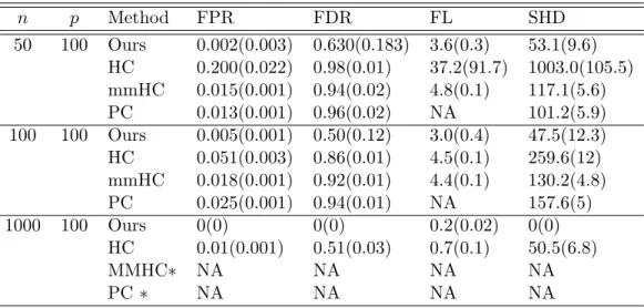
Table 2.2: Averaged false positive rate (FPR), false discover rate (FDR), Frobenius norm loss (FL), and Structural Hamming Distance (SHD), as well as their standard errors (in parenthesis), for four competing methods based on 100 simulation replications in Example 2. Here “Ours”, ”HC”, ”MMHC” and ”PC” denote ours, the HC, the MMHC and the PC methods. Note that N/A means that a method does not yield parameter estimation. Here∗represents no return value after 24 hour running time. n p Method FPR FDR FL SHD 50 100 Ours 0.002(0.003) 0.630(0.183) 3.6(0.3) 53.1(9.6) HC 0.200(0.022) 0.98(0.01) 37.2(91.7) 1003.0(105.5) mmHC 0.015(0.001) 0.94(0.02) 4.8(0.1) 117.1(5.6) PC 0.013(0.001) 0.96(0.02) NA 101.2(5.9) 100 100 Ours 0.005(0.001) 0.50(0.12) 3.0(0.4) 47.5(12.3) HC 0.051(0.003) 0.86(0.01) 4.5(0.1) 259.6(12) mmHC 0.018(0.001) 0.92(0.01) 4.4(0.1) 130.2(4.8) PC 0.025(0.001) 0.94(0.01) NA 157.6(5) 1000 100 Ours 0(0) 0(0) 0.2(0.02) 0(0) HC 0.01(0.001) 0.51(0.03) 0.7(0.1) 50.5(6.8) MMHC∗ NA NA NA NA PC∗ NA NA NA NA

(32)

by the SHD, the proposed method performs the best in Example 2, and slightly worse than the MMHC algorithm in Example 1. The HC algorithm and our method gives relatively robust results across two examples. However, the performance of the HC is not satisfactory. The poor performance of HC may be partly due to inappropriate use of the BIC for the model selection in a high-dimensional situation. while the PC and the MMHC, which relies on the PC, do not deliver robust performance across the examples. PC and MMHC perform well in Example 1 but lead to deteriorated performance in Example 2, where the non-sparse neighborhood of the “hub” node becomes the curse of the two methods. Moreover, in the case n = 1000 in Example 2, the PC and the MMHC fail to return a solution after 24 hour running time. In contrast, the proposed method gives consistent performance in Example 2 with the smallest FPR, PFD and SHD values and a large amount of improvement over other competing methods.

With regard to accuracy of parameter estimation, the proposed method performs best in most cases except one case with a large sample size (n= 1000 and p = 100) in Example 1, as measured by the Frobenius norm loss.

Overall, the proposed method compares favorably against top performers in the literature.

2.5.2 Oracle properties

In this simulation study, we demonstrate the theoretical result in Theorem 2 that the proposed method is able to correctly identify the oracle estimator asymptotically. There are two purposes for this. First, the simulation will demonstrate that the asymptotic property can be realized in a finite-sample situation. Second, an concordance between our and the oracle estimators indicates that our DC algorithm yields a global optimizer, because the oracle estimator is in fact the global optimizer of our nonconvex problem in certain sense. For comparison, HC, MMHC and PC are included. Still, the PC algorithm does not yield parameter estimation.

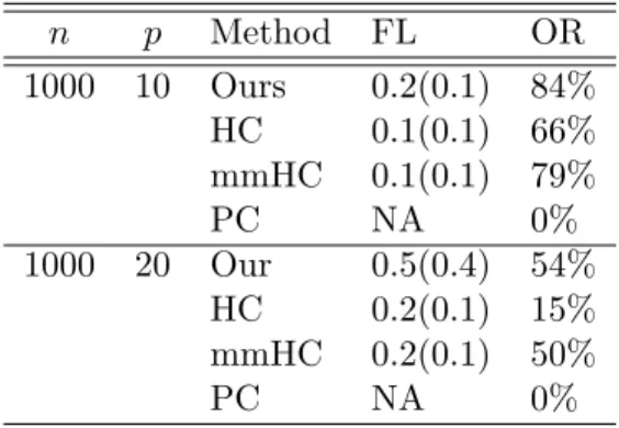
As in the setting of Example 1, we randomly generate a DAG withp= 10,20 nodes, with the number of edges equal to the number of nodes. As suggested by Table 3, the proposed method has a good agreement rate of 54% and 84% for n = 1000 and p = 10,20. This says that it has a good probability of 54% and 84% to yield a global optimizer in these cases. This aspect of a DC algorithm agrees with the finding of [30]

(33)

for a different problem.

Table 2.3: Frobenius norm loss (FL), and oracle rate (OR) for three competing methods based on 100 simulation replications in Example 3. Here “Ours”, ”HC”, and ”MMHC” denote ours, the HC and the MMHC. n p Method FL OR 1000 10 Ours 0.2(0.1) 84% HC 0.1(0.1) 66% mmHC 0.1(0.1) 79% PC NA 0% 1000 20 Our 0.5(0.4) 54% HC 0.2(0.1) 15% mmHC 0.2(0.1) 50% PC NA 0%

2.5.3 An example demonstrating consistency

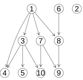
Similar to the setting of Example 1, we randomly generate a DAG with p= 10 nodes, as depicted in Figure 2.1. In this case, we study accuracy of reconstructing a DAG’s structure of the proposed method, HC and MMHC as a function of the sample size n while p= 10 is held fixed. Note that the DAG is fully identifiable. Furthermore, PC is not considered because it only gives partially directed graphs. The results are displayed in Figure 2.2 for n= 20,100,500.

Asn increases fromn= 20 ton= 500, the proposed method continues to improve until identifying all directions correctly. By comparison, HC and the MMHC recover the true skeleton but miss several directions, which remains missed asn increases.

(34)

1

2

3

4

5

6

7

8

9

10

Figure 2.1: DAG representation of the true network in Section 5.2.

2.5.4 Analysis of cell signaling data

This section applies the proposed method to analyze multivariate flow cytometry data in [44]. Data were collected after a series of stimulatory cues and inhibitory interventions, with cell reactions terminated 15 minutes after stimulation by fixation, to profile the effects of each condition on the intracellular signaling networks of human primary naive CD4+ T cells. 7466 flow cytometry measurements were made over eleven phosphory-lated proteins and phospholipids from nine experimental conditions. The primary goal of this experiment is to infer causal influences in cellular signaling networks through perturbations with molecular interventions. This requires a multivariate in lieu of uni-variate approach, which is possible given the simultaneous measurements. Note that the data is interventional from nine experiments whereas our method and the other three are designed for observational data. Therefore, we centered data from each experiment separately before combining them to remove intervention effects on means so that the data becomes more observational.

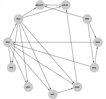
This is a well-studied example and we use the representation in Figure 3.1 from [44] as a benchmark. A direction from one node to another is interpreted as a directional influence between the corresponding two proteins. The reader may consult [44] for details about the data.

(35)

Ours with n= 20 ● ● ● ● ● ● ● ● ● ● 1 2 3 4 5 6 7 8 9 10 HC with n= 20 ● ● ● ● ● ● ● ● ● ● 1 2 3 4 5 6 7 8 9 10 MMHC with n= 20 ● ● ● ● ● ● ● ● ● ● 1 2 3 4 5 6 7 8 9 10 Ours with n= 100 ● ● ● ● ● ● ● ● ● ● 1 2 3 4 5 6 7 8 9 10 HC with n= 100 ● ● ● ● ● ● ● ● ● ● 1 2 3 4 5 6 7 8 9 10 MMHC with n= 100 ● ● ● ● ● ● ● ● ● ● 1 2 3 4 5 6 7 8 9 10 Ours with n= 500 ● ● ● ● ● ● ● ● ● ● 1 2 3 4 5 6 7 8 9 10 HC with n= 500 ● ● ● ● ● ● ● ● ● ● 1 2 3 4 5 6 7 8 9 10 MMHC with n= 500 ● ● ● ● ● ● ● ● ● ● 1 2 3 4 5 6 7 8 9 10

Figure 2.2: Reconstructed networks by various methods. True and false discoveries are marked with green and red lines, where wrong directions are considered to be false in this case.

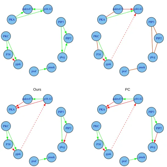
We fit (2.4) with one tenth samples for training and nine tenths for tuning. The learned networks are shown in Figure 2.4. An edge is marked in green if it matches one in Figure 3.1; otherwise it is red, including wrong orientation cases. If an edge does not even match the skeleton in Figure 3.1, then it is marked in dashes. All four methods give similar results due to the large sample size relative to the number of nodes. The proposed

(36)

method identifies nine true edges, one wrong edge. All the other three methods have more false discoveries. In addition, the PC has fewer correct directions. Unfortunately, however, all methods miss several known edges. One possible reason is that many directional relations in protein-signaling networks may behave nonlinearly, which can not be captured by a linear model. Analysis based on discretization data [44, 19] tends to capture such nonlinearity and thus more true edges. Another possible reason is that we removed, before the analysis, intervention effects, which may be crucial in identifying directional relations. Incorporating interventional data is one future direction to extend our method. PIP2 pmek p44.42 PKC pjnk pakts473 PKA praf plcg PIP3 P38

Figure 2.3: Display of a consensus protein network consisting of eleven proteins.

2.6 Discussion

This article proposes a method for reconstructing the graphical structure of a directed acyclic graph. The method identifies the true DAG by estimating the adjacency matrix of the graph using a constrained likelihood maximization incorporating acyclicity of a DAG through constraints.

(37)

Ours PIP3 plcg PIP2 PKC PKA praf P38 pjnk pmek p44.42 pakts473 PC PIP3 plcg PIP2 PKC PKA praf P38 pjnk pmek p44.42 pakts473 HC PIP3 plcg PIP2 PKC PKA praf P38 pjnk pmek p44.42 pakts473 MMHC PIP3 plcg PIP2 PKC PKA praf P38 pjnk pmek p44.42 pakts473

Figure 2.4: Reconstructed networks using the proposed method and the other three methods. Correct discoveries are marked in green, whereas false discoveries are displayed in red. The network constructed by the PC is partially directed.

For reconstruction of directional relations, we introduce a method that is dramati-cally different from conventional methods to overcome two major difficulties. The first concerns super-exponentially many constraints, which is addressed by a novel constraint reduction method reducing to cubic in the number of nodes. The second is identifia-bility of directional relations. The proposed method enables us to reconstruct all the

(38)

directional relations when possible through the acyclicity constraints.

The proposed method, particularly the idea of identifying active constraints from super-exponentially many constraints, may be useful and generalized to other problems, especially for nonlinear models. Further investigation is necessary.

(39)

Chapter 3

Maximum likelihood estimation

of multiple directed acyclic

graphs

In this chapter, we go beyond the single DAG reconstruction discussed in Chapter 2 and propose a constrained likelihood approach to learning multiple DAGs from inho-mogeneous data. Another deviation from Chapter 2 is that we assume the ordering of nodes is known. The rest of this chapter is organized as follows.Section Section 3.1 introduce the background of DAG learning when the ordering is known. 3.2 introduces the methodology, followed by our computational development in 3.3. Operating char-acteristics of the proposed method are examined on simulated and real data in Sections 3.4 and3.5, respectively.

3.1 Background

Reconstruction of a DAG given a partial ordering is equivalent to sparse estimation of Cholesky decomposition of a covariance matrix, and thus is computationally fea-sible [22]. The ordering information is usually determined by a natural ordering of temporal observations, previous experiments and prior knowledge. In this article, we

(40)

reconstruct multiple DAGs given a known partial ordering. To our knowledge, estima-tion of structural changes over multiple DAGs has not been yet explored, although that over multiple undirected graphs has been studied in [45, 46, 47]. In practice, identifica-tion of a change in causality structure arises from detecting a change corresponding to that of experimental conditions or responding to a certain event or treatment.

This chapter focuses on maximum likelihood estimation of multiple DAGs under a structural equation model. It is known that maximum likelihood estimation breaks down when the number of variables exceeds the sample size. Even for a moderately sized problem, it always yields a complete graph and does not estimate graphical structures well. Therefore, different methods using penalization have been proposed for sparse estimation of graphical models [48, 49, 36, 22]. To achieve our goal of learning graphical structures, we construct two nonconvex constraints based on the truncatedL1-function

(TLP, [7]), as a computational surrogate of the L0-function, with one constraint

im-posing sparseness and the other encouraging a common structure. Computationally, with difference convex programming and augmented Lagrange multipliers, nonconvex minimization is solved through a sequence of convex subproblems iteratively. For each subproblem, we develop a fast algorithm to treat a constrained L1-problem, which we

call pairwise coordinate descent algorithm.

3.2 Statistical methodology

Given L p-dimensional vectors of random variables X(l) _{= (}_X(l)

1 , . . . , X (l)

p )T with a

known partial ordering, one from each population, we use L DAGs to describe causal relations within each population and to explore differences among the populations. That is, each component X_i(l) corresponds to one node in the lth DAG, with a directed edge between two nodes indicating a causal relation between them. Without loss of generality,we assume that X(l) has been sorted according to its partial order, which means a causal relation is only possible from X_i(l) toX_j(l) fori < j.

To model causality among the components of X(l)_{, consider a structural equation}

model of the form

(41)

whereA(l) is an adjacency matrix in which a nonzerojk-th element ofA(l)corresponds to a directed edge from parent node k to child note j with its value A(_jkl) indicating the strength of the relationship, and (l) = (₁(l),· · · , (pl))T is an independent latent

variable vector representing unexplained variations in the nodes and acting as random noises. Note that A(_i,jl) = 0 for i < j, since X(l)’s are assumed to be ordered. In addition, A(_iil) = 0, for all i, as a self-loop is not allowed in a DAG. Therefore, the adjacency matrices A(l),l= 1, . . . , L, are lower triangular with zero diagonal elements, that is, A(_i,jl) = 0, j ≥ i. The model basically says that each X_j(l) depends linearly on its parent variables and some latent variable (_jl). Here we assume that ₁(l),· · · , (pl)

follow independent normal distributions, that is, (_jl) ind∼ N(0,(σ(_jl))2). This implies that X(l)’s follow multivariate normal distributions. Note that (3.1) becomes Gaussian autoregressive model when the subscript of X_i(l) denotes the consecutive time. Our likelihood method is readily generalizable to other distributions. The reader may consult [50] for (3.1) and structural equations.

In (3.1), nonzero entries of A(l) _{are uniquely specified by the} _l_{th DAG. Thus, we}

estimate (A(1), . . . ,A(L)) to preserve a common structure and identify differences among them.

For a total of n = PL

l=1nl random samples, nl samples are drawn according to

(3.1) for each l to form an n×p data matrix X(l) = (x₁(l), . . . ,x(pl)), where eachx(_jl) =

(x(₁l_,j), . . . , x(_nl)

l,j)

T _{is an} _n

l-dimensional column vector for each node, and samples from

different populations X(l)are assumed to be independent. Note that an arbitrary mean vector can be incorporated by adding an intercept to (3.1).

Let k−={j = 1, . . . , k−1} be a set of indices, with k = 1 indicating the null set. Let X(_jl−) = (x (l) 1 , . . . ,x (l) j−1), A (l) j,j− =

A(_j,l₁), . . . , A_j,j(l)₋₁. The likelihood of X(l) can be written as fX(1), . . . ,X(L)= L Y l=1 fX(l)= L Y l=1 p Y j=1 fx(_jl)|X(_jl−) = p Y j=1 L Y l=1 fx(_jl)|X(_jl−) . (3.2)

(42)

−logf X(1), . . . ,X(L) = p X j=1 L X l=1 −logf x(_jl)|X(_jl−) ! . (3.3)

Using the fact that X_j(l)|X_j(l−) follows N A(_j,jl)−X (l) j−,(σ (l) j )2

from (3.1), we obtain that

−logf X(1), . . . ,X(L) = p X j=1 L X l=1 1 2(σ_j(l))2 x(_jl)−X(_jl−) A(_j,jl)− T 2 +njlogσ_j(l) !! . (3.4) Maximizing (3.2), equivalently minimizing (3.4), may result in over-fitting and lead to fully connected DAGs, especially when the number of unknown parameters exceeds the sample size. We therefore regularize (3.3) through nonconvex constraints to pursue sparsity and detect structural changes. Note that the constrained approach is not equivalent to its penalized regularization counterpart because of nonconvexity in this case.

Our method is to regularize the number of nonzeros of the adjacency matrices as well as the number of pairwise differences between the corresponding entries across adjacency matrices. Let L be a set of index pairs in which a pair (l, s) indicates the possibility that A(l) andA(s) share some common entries and can be grouped or collapsed if data suggest so. Constraints are used to regularize, which are in the form:

L X l=1 kA(l)k0 ≤t1, X (l,s)∈L kA(l)−A(s)k0≤t2. (3.5)

wherekAk0:=Pp_i₌₁Pp_j₌₁I(|Ai,j| 6= 0), is theL0-norm ofA, or the number of nonzero

entries of A, t1 ≥ 0 and t2 ≥ 0 are tuning parameters corresponding to the number

of nonzeros of the adjacency matrices and the number of element-wise differences with respect to L. A complete set L = {(l, s) : 1≤ l < s ≤L} is used unless additional information is available. For example, a temporal set L ={(l, l+ 1) : 1 ≤l≤L−1}

is used in dynamic networks with l representing consecutive times.

To allow for different degrees of sparsity over different rows of lower triangular matrices A(l), we replace (3.5) by p pairs of row-wise sparsity through 2p different tuning parameters {t1,j, t2,j}:

(43)

L X l=1 j−1 X k=1 A (l) j,k 0≤t1,j, X (l,s)∈L j−1 X k=1 A (l) j,k−A (s) j,k 0≤t2,j, j= 1,· · · , p. (3.6)

This is computationally feasible because the log-likelihood (3.3) is separable or decom-posable in j. In fact, minimizing (3.3) subject to (3.6) reduces top subproblems.

To circumvent computational difficulty of minimizing (3.3) subject to (3.6), we ap-proximate theL0 funtion there by a surrogate function, the truncatedL1function (TLP,

[7]), defined as Pλ(x) = min

_|

x|

λ,1

. Asλtends to 0, the TLP recovers theL0-function

exactly. Now the constraints in (3.6) become

L X l−1 j−1 X k=1 Pλ(A (l) j,k)≤t1,j, X (l,s)∈_L j−1 X k=1 Pλ(A (l) j,k−A (s) j,k)≤t2,j, j= 1,· · · , p. (3.7)

To simplify tuning, we introduce a single constraint for each row as opposed to the two constraints in (3.7), with new tuning parameters (κj, tj) corresponding to (t1,j, t2,j),

L X l=1 j−1 X k=1 Pλ(A(j,kl)) +κj X (l,s)∈_L j−1 X k=1 Pλ(A(j,kl) −A (s) j,k)≤tj j = 1, . . . , p, (3.8)

where κj seeks a trade-off between sparsity and grouping.

Based on the foregoing discussion, we solve (3.3) subject to (3.8) by solving its equivalent form through psubproblems:

min L X l=1 1 2(σ(_jl))2 x(_jl)−X(_jl−) A(_j,jl)− T 2 +nllogσ_j(l) ! , subject to L X l=1 j−1 X k=1 Pλ(A(_j,kl)) +κj X (l,s)∈L j−1 X k=1 Pλ(A(_j,kl) −A_j,k(s))≤tj, j= 1, . . . , p. (3.9)

These p subproblems are of the same type, hence we only need to consider a general form. Let Y(l) _{be a vector of length} _n

l, corresponding to x(jl) in (3.9), X(l) be an nl

by m matrix, corresponding toX(_jl−) withm =j−1, andβ(l) be m-dimensional vector corresponding to A(_j,jl)−. Then, a general form is,

(44)

min L X l=1 1 2σ2 l kY(l)−X(l)β(l)k2+nllogσl , subject to L X l=1 m X j=1 min |β (l) j | λ ,1 ! +κ X (l,s)∈L m X j=1 min |α (ls) j | λ ,1 ! ≤t. (3.10) where α(_jls) =β(_jl)−β_j(s), and ζ = (β_j(l)j=1,...,m l=1,...,L, α (ls) j (l,s)∈_L

j=1,...,m) is our new set of variables

to be optimized. In addition, a new constraint T ζ = 0 is imposed, namely,β_j(l)−β_j(s)−

α(_jls)= 0, forj = 1, . . . , m, (l, s)∈L.

3.3 Computation

This section develops a computational method for nonconvex minimization (3.10) through difference convex programming, augmented Lagrange multipliers and our pairwise co-ordinate descent algorithm.

3.3.1 Difference convex programming

For minimization in (3.10), we employ difference convex (DC) programming, which leads to a finite-step termination due to piecewise linearity of the TLP function [7]. Here Pλ

can be decomposed into a difference of two convex functions:

Pλ(x) = min _| x| λ ,1 = |x| λ −max _| x| λ −1,0 . (3.11)

This in turn yields a decomposition of the left-hand side of (3.10) into a difference of two convex part, that is,