1
Review
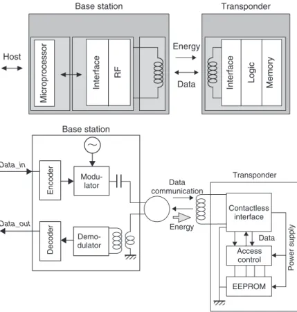
Before going into the details, let us briefly review how the components of an RFID system are organized and how they operate.Figures 1.1a and1.1bshow the structure of a system of this kind.
Base station Host Microprocessor Interface RF Energy Data Transponder
Interface Logic Memory
Base station Data_in Data_out Encoder Modu-lator Decoder Demo-dulator EEPROM Access control Data Power supply Contactless interface Energy Data communication Transponder
Figure 1.1a Block diagram of a contactless system
Note: for more detailed information, you should refer to the author’s very compre-hensive book on the subject, published previously by Dunod.
RFID and Contactless Smart Card Applications D. Paret 2005 John Wiley & Sons, Ltd
Magnetic field lines
Energy
Coil axis Transponder
Data
Antenna
Figure 1.1b Operating principle of a “base station – transponder” system
1.1 The Elements of a Contactless Device
1.1.1 The transponder
Let us start with the transponder, which uses a remote memory (ROM, PROM, E2PROM, etc.) to store data for the application in question, and which also controls communication and contains the part used for the RF link.
1.1.2 The air interface
The air forms the communication medium. The electromagnetic RF waves carry the data. The air also plays a part in the (magnetic) coupling between the antennae of the transponder and the base station.
1.1.3 The base station
The base station comprises an analogue part used for receiving and transmitting RF signals, the circuits controlling the protocol for communication with the transponder, the communication management (management of possible collisions, authentication, cryptography, etc.) and finally an interface for dialogue with the host system.
1.1.4 The host system
Finally, to complete this brief survey, we have the host system, providing the higher level control of the application.
Now that the general picture is in place, let us examine each of these elements in more detail.
1.2 General Operating Principles of the ‘‘Base
Station–Transponder’’ Pair
For applications in which the remote element – the transponder – has no on-board power supply and therefore operates with a remote power supply,Figures 1.2a to1.2c provide a summary of the physical principles of the three main stages of operation of a “base station–transponder” system.
1.2.1 Transfer, energy supply and remote power supply
An alternating electrical signal at radio frequency, called the “carrier”, creates a mag-netic field, by means of the winding forming the base station antenna, to remotely induce a voltage in the antenna of the transponder; this voltage is rectified and filtered to provide a local power supply for the transponder (seeFigure 1.2a).
Ub Ut
lb
lt
Energy
Figure 1.2a Energy transfer phase
1.2.2 Data transfer from the base station
to the transponder: the ‘‘uplink’’
In order to transmit commands and data to the transponder, the carrier is modulated with a binary stream based on specific bit codings (seeFigure 1.2b).
Demodulator l Energy Data lb lt Ub Ut Data
Figure 1.2b Uplink phase
1.2.3 Data transfer from the transponder to the base
station: the ‘‘downlink’’
The transponder can communicate with the base station by means of a modulation carried out by varying the load that it represents in the field (seeFigure 1.2c).
lb lt Ub Ut Energy Data Demodulator VZ1 VZ2 (VZ2<VZ1) Data
To explain the operation of the “base station–transponder” pair more simply, I shall look inside most of its constituent parts and try to explain the general principles as clearly as possible, breaking the process down into two main sections, namely, the transfer of energy on the one hand and the operation of the uplink and downlink on the other.
1.2.4 Energy transfer
The transponder can only operate if it is supplied with power. In the present case, this is done by the remote power supply principle, which will be described in detail in this section.
Figure 1.3 shows how the energy transfer is carried out by means of an alternating magnetic fieldH(t) produced by the flow of an alternating currentI(t) in the antenna of the base station, according to the general equation
H =NI,
whereNrepresents the number of turns per metre of the antenna carrying the currentI. The strength of the magnetic fieldH is expressed in amperes per metre (A/m).
Magnetic field lines
Energy
Antenna axis Transponder
Data
Antenna
Figure 1.3 Energy transfer
In the medium in which this magnetic field develops, there is a corresponding associated inductionB(t) having the general form
B(t)=µ H (t),
where µ represents the magnetic permeability of the medium(s) through which the field passes. This magnetic permeability is expressed by
where µ0 represents the permeability of the air (µ0 =4π×10−7 henrys/metre) and
µr is the relative permeability of the medium concerned (water, metal, etc.). The value of the magnetic inductionB is expressed in teslas (T).
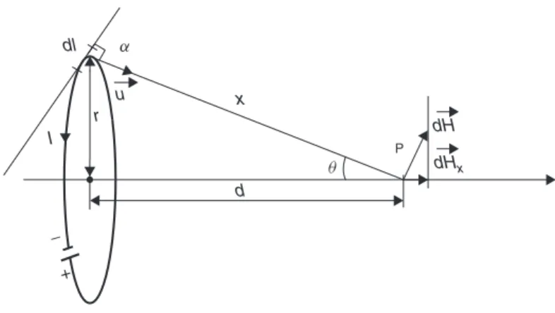
The Biot–Laplace and Biot–Savart laws establish the relationship between the cur-rentI flowing in an elementdl of an electrical circuit having a lengthland the intensity of the magnetic inductionB as a function of the distancexbetween the measurement point (of unit vectoru) and the elementdlproducing the field according to the formula:
−→ dH = (I · −→ dl)∧ u 4π(x2) Therefore, B=µH = (µI ) 4π −→ dl∧ u x2
where is a line integral calculated over the whole lengthl and ∧is the notation of the vector product.
−→ dH = (I· −→ dl)∧ u 4π x2 ⇒dH = I·dl·sinα 4π x2 Now, α= π 2 ⇒sinα=1 and therefore dH = I ·dl 4π x2 In the axis of the coil, we find
dHx = I 4π x2 dlsinθ Now, x= r sinθ and therefore dHx = 1 4π r2sin 3 θdl
On the other hand, at a distance d in the axis of the coil, (seeFigure 1.4)
x=r2+d2 and
sin3θ = r
3
dH dHx P q x d dl a I + − u r
Figure 1.4 Magnetic field strength as a function of distance and antenna radius
and therefore sin3θ = r 3 (r2+d2)3/2 This gives us dHx = 1 4π · r (r2+d2)3/2dl ⇒Hx = I 4π · r (r2+d2)3/2 2π r 0 dl = I r 2 2(r2+d2)3/2 Solving this equation for a circular base station antenna with the radiusr having a flat configuration, withN turns, at a point P located at a distanced along the axis of the antenna, we find:
B(d, r)=µ r
2
2[(r2+d2)3/2]NI =µ·H (d, r) Examples, in air, withµ=µ0=4×3.14×10−7:
−ifH =1 A/m, thenB =µ0H =1.256µT; −if B=1µT, thenH = B
µ0 =
0.796 A/m.
NOTE
To ensure that the following chapters are understood, it will be useful to review the following concepts, which are in fact simply different aspects of the equation shown above.
B(d) atr=constant
It is useful to examine the variations of magnetic induction as a function of the distance between the base station antenna and the transponder, since there are numerous applications for which the radius of the base station antenna is constant and the distance between the base station and the transponder is variable (e.g. ticket presentation, access control, object identification, etc.). We shall therefore examine in detail the general equation of magnetic induction,
B(d, r)=µ r
2
2[(r2+d2)3/2]NI
assuming in this case that the value ofr is constant. It is therefore a functionB(d). To investigate its variations, we calculate its derived functionB(d), which is of the type−v/v2. After expansion and reduction, we have
B(d)= −3(µNI)r
2
2 ·
d (r2+d2)5/2
This first derivativeB(d)is cancelled ford=0, andB(d,r) has a maximum with the value
B(d =0)=Bmax=
(µNI)
2r
Now we calculate the second derivativeB(d) to determine whether any points of inflection are present. This derivative is of the type(uv−vu)/v2. After expansion and reduction, we have
B(d)= −3(µNI)r
2
2 ·
r2−4d2 (r2+d2)7/2
This second derivative B(d) is cancelled for 4d2=r2, signifying that the curve of the variations of B(d) therefore has two symmetrical points of inflection for d =
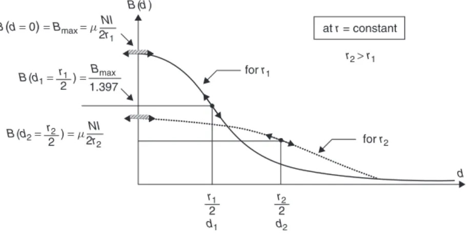
±(r/2). B d= r 2 =µ 1 2r 5 4 3/2NI =B(d=0) 1 5 4 3/2 = B(d1.397=0)
The curve of the variations ofB(d) for a constant radius of the base station antenna is shown inFigure 1.5.
In this figure, these variations are deliberately shown with respect to two differ-ent radii of the antenna, r1 and r2, where r2> r1, to illustrate the content of the following text.
Still considering B(d) for a constant radius, we shall now examine two common cases of application.
B(d = 0) =Bmax =m B(d1= ) = NI 2r1 NI 2r2 Bmax 1.397 r1 2 B(d2= ) r22 =m r1 2 d1 r2 2 d2 B(d) for r1 for r2 r2 > r1 at r = constant d
Figure 1.5 Variation ofB(d) with constant radius of base station antenna Operation of the transponder at a specified distance
If the transponders have to operate at a specified distance d1, it will be necessary to produce a closely specified magnetic inductionB(d1), which, having a constant product (NI), will be obtained for a specified value ofr1.
Operation of the transponder in a specified range of distances
We shall now examine the case in which transponders are required to operate, not at a fixed distance from the base station but within a specified range of distances. In this case, to obtain the greatest possible reproducibility of operation, it is generally desirable for the transponder to be exposed as far as possible to a magnetic inductionB that is, “virtually” constant over the desired range of distances. To do this, as indicated in the figure, the curve representing the variations of magnetic induction B as a function of the distanced must be as flat as possible over the range of distances fromd1 tod2.
In this case, still with a constant product (NI), it is preferable to increase the value
r of the radius of the antenna, since, even if the maximum induction decreases as a result, in the range of distancesd1,d2, its variations change more slowly as a function of the distance. In this type of application, the designer must therefore calculate the literal expressions of B(d1) and B(d2)– with r as the parameter – to enable him to determine the exact value ofr that minimizes the difference=B(d1)−B(d2).
We should note in passing that the “delta” () equation takes into account the variables r, d1 and d2 (where d2 =d1+const) and that at a desired value of the value of r will depend on d1 and on const, in other words on the two parameters “initial minimum distance and desired range of distances”, and not solely on the value of the desired range.
B(r)at d=constant
It is also useful to examine the variations ofB(r) atd=constant, since this repre-sentative case is found in many applications where the operating distance between the base station and transponders is constant (e.g., in the identification of objects moving on a conveyor in a production line).
We shall now examine the general equation for magnetic induction, to find the optimal value for the radius of the base station antenna for this kind of application.
Returning to the general equation,
B(d, r)=µ r
2
2[(r2+d2)3/2]NI
let us now assume that in this case the value ofd is constant. It is therefore a function
B(r).
To study its variations, we calculate its derived function B(r), which is of the type
(uv−vu)/v2.
After expansion and reduction, we have
B(r)= µNI
2 ·
r(2d2−r2) (r2+d2)5/2
This derivative is cancelled forr =0 and forr= ±d√2= ±1.414d.
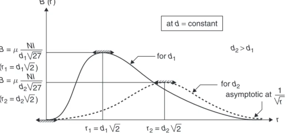
Examining the changes of signs in this derivative, we see that B(r) passes through a minimum at r =0 (which was physically predictable, since B(r=0)=0!) and through a maximum forr = ±1.414d. The value of this maximum is
(r =1.414d)=µNI 1
d√27
The curve of the variations of B(r) at the distance d=constant is shown in Figure 1.6. B = m NI d1 27 B = m NI d2 27 2 (r1 = d1 ) 2 r1 = d1 2 (r2 = d2 ) r 2 r2 = d2 at d= constant for d1 for d2 asymptotic at B (r) d2 > d1 r 1
Figure 1.6 Variation ofB(r) with constant distanced
Now you know what needs to be done to optimize a system operating at a fixed distance. Everything else being equal, if you specifyr =1.414d you will obtain the greatest induction; alternatively, for a given induction, you simply decrease the value of the currentI to obtain it.
Rationalized equation of induction B(d,r) To generalize the argument con-cerning the relative values ofd andr, we shall now rationalize this general magnetic
field strength or magnetic induction equation. To do this, we assume that d=a·r. The general equation then takes the form
B(a, r)=µ 1
[(1+a2)3/2]· NI
2r =µ·H (a, r)
Now, the valueNI/2rrepresents the value ofH (a, r)fora=0, that is,H (0, r)in the centre of the flat circular antenna, and therefore
H (a, r)= 1
(1+a2)3/2H (0, r)
We can now look at some specific examples according to the relative values of r
andd or values of the ratioa=d/r.
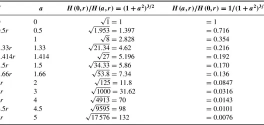
Table 1.1 shows, for a given value ofr, the values of the correction factor(1+a2)3/2
and its reciprocal as a function of the ratioa=d/r.
Table 1.1 d a H(0,r)/H(a,r)=(1+a2)3/2 H(a,r)/H(0,r)=1/(1+a2)3/2 0 0 √1=1 =1 0.5r 0.5 √1.953=1.397 =0.716 r 1 √8=2.828 =0.354 1.33r 1.33 √21.34=4.62 =0.216 1.414r 1.414 √27=5.196 =0.192 1.5r 1.5 √34.33=5.86 =0.170 1.66r 1.66 √53.8=7.34 =0.136 2r 2 √125=11.8 =0.0847 3r 3 √1000=31.62 =0.0316 4r 4 √4913=70 =0.0143 4.5r 4.5 √9595=98 =0.0101 5r 5 √17 576=132 =0.0076
Very near field (d r, or a1) If the distanced between the base station antenna and the transponder is very small compared with the radius r (dr, that is, has a very small value ofa), the transponder is in the “very near field” of the transmitting antenna and the equation takes a form of the type const/r and the induction B(d) changes to 1/r.
Note that ford=0 (anda=0), we return to the well-known formula for induction in the centre of a flat circular coil:
B(0, r)=µNI
2r =µ·H (0, r)
Near field (d of the order of r, or a of the order of 1) The special case whered=r
(a=1) is frequently encountered in contactless applications. In this case, the value of
B(d, r)becomes B(d, r)=µ 1 2r√8NI = B(0) √ 8
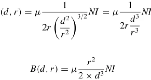
Near field (d>r, or a>1) If the distance d is large (but not enormously large!) with respect to the radius of the antennaa (e.g. a=2,3, . . . ,5, . . .), the transponder is still in the “near field” of the transmitting antenna. The value ofa2 is therefore large with respect to 1, and the equation is reduced to the form
B(d, r)=µ 1 2r d2 r2 3/2NI =µ 1 2rd 3 r3 NI and therefore B(d, r)=µ r 2 2×d3NI
and for a specific constant value ofrit takes a form of the type const/d3. The induction
B(d) then changes to 1/d3.
By way of a summary, Figure 1.7 shows the trend of the variations of the general functionB=f (d), in the very near and near fields, wherer is constant.
B mH H NI or 1 2r max = max / 8 max / 125 max / 1000 at r= constant r 2r 3r 4r d × × ×
Figure 1.7 General variation ofB(d) (near and far fields)
Far field (d≫r, or a≫1) In Chapter 6 we shall examine in detail what are known as far (or very far) fields, in other words those in whichd≫r, which, as we will show, are no longer subject to the Biot and Savart law but relate to the standard propagation of radio waves.
In this case, the predominance of the fieldH is reduced, and radiated fields Eand
H are present.
1.2.5 Remote power supply
The principle of the remote power supply to the transponder will now be summarized. The magnetic inductionB causes the appearance of a magnetic flux. At a distance
d, in a conductor having a total cross section S=N·s (where N is the number of turns), this flux is equal to=B(d)·S.
The instantaneous variation of magnetic flux causes the appearance of an induced potential difference (pd),u(t), across the terminals of the conducting element acting as the receiving antenna, which is affected by the variation of the flux according to the well-known equation
u(t)= −d
dt .
That is the essential description of the appearance of a pd across the terminals of the transponder antenna, corresponding to an inductionB present in the vicinity of the transponder, generally ranging from a few tens of nanoteslas (nT) to a few hundred microteslas (µT).
When the transponder has been tuned to the carrier frequency by means of tuned resonant circuits of the LC type, a voltage (derived from this induced voltage) of the order of several volts will be applied to the terminals of the integrated circuit.
The next step is to rectify this incident-induced alternating sinusoidal voltage, to recover a unidirectional voltage, after which it must be filtered and regulated to provide a continuous voltage, using filter capacitors whose values are, evidently, functions of the received carrier frequency (e.g., of the order of a nanofarad (nF) for 125 kHz, or several tens of picofarads (pF) for 13.56 MHz).
The quality and quantity of the energy transfer depend on the frequencies to which the two antenna circuits (base station and transponder) are tuned; their precision, tol-erances, fluctuations and so on; the coupling coefficient (distances, geometrical shape of the antennae, etc.); and, of course, the quality factors of the tuned circuits of the base station and transponder.
However, if everything else is equal, the critical value – the threshold – for a good supply is achieved and corresponds on the one hand to a certain minimum induction
Bmin but also, on the other hand, to a particular magnetic coupling (which of course depends on the distance, among other factors) related to the possibility of providing a sufficient quantity of energy, which will be denotedke.
1.2.6 Communication between the base station
and transponder
We shall now look at the exchanges that have to take place between the base station and transponder, and more precisely the exchanges from the base station to the transponder, which will be referred to as the “uplink”, and those from the transponder to the base station, known as the “downlink”.
NOTE
The technical literature provides many definitions of the “direction” of the “uplink” and “down-link”. In this book, it is simply assumed that the base station system supplying energy to the transponder is the reference point of the system, and that the links originating from the base station are “uplinks”.
The uplink In the upward direction, the base station communicates with the transponder by means of a coding (binary) and a carrier modulation system that must not affect (or must only slightly affect) the quality of its remote power supply function.
In this case, the value of the couplingkeis sufficient to provide the remote energy and power supply to the transponder, and also to provide the uplink for the communication between the base station and the transponder.
The downlink In the downward direction, from the transponder to the base station, the transponder must be able to communicate with the base station. The technical principle implemented in most commercially available transponders is that of “load modulation”. The most widely used principle is that of a type of modulation based on a variation of resistive load.
By varying this load, the transponder modifies the energy consumption that it rep-resents in the magnetic field and, because of the magnetic coupling between the transponder and the base station, tends to modify the current flowing in the circuit of the base station antenna.
Minimum coupling I have written “tends to modify”, rather than “modifies”. This is because, in order for this modulation/load variation of the transponder to be sensed and detected in the base station circuits used for this purpose, it is necessary for a minimum magnetic couplingkapplicationto be present between the transponder and the base station antenna. We must distinguish between the concept of the coupling required for the energy transferkefor the remote power supply of the transponder and the coupling required to establish the downlink to enable the application to operate correctlykapplication.
1.3 Before We Continue
. . .
Conventional
Notation
Before we continue, let me summarize the conventional notation used throughout the book:
• subscript 1 for everything relating to the base station (the “primary” physical event);
• subscript 2 for everything relating to the transponder (the “secondary” physical event);
• a lower-cases for everything relating to “serial” physical representations;
• a lower-casep for everything relating to “parallel” physical representations;
• lower-case letters for instantaneous values or values of the complex variable;
• upper-case letters for values of permanent or rms parameters.
NOTE
In order to avoid cumbersome arrays of symbols when explaining specific points, I have sim-plified the notation (which is still adequate, and certainly much clearer).