HAL Id: hal-01544239
https://hal.archives-ouvertes.fr/hal-01544239
Submitted on 21 Jun 2017
HAL
is a multi-disciplinary open access
archive for the deposit and dissemination of
sci-entific research documents, whether they are
pub-lished or not. The documents may come from
teaching and research institutions in France or
abroad, or from public or private research centers.
L’archive ouverte pluridisciplinaire
HAL, est
destinée au dépôt et à la diffusion de documents
scientifiques de niveau recherche, publiés ou non,
émanant des établissements d’enseignement et de
recherche français ou étrangers, des laboratoires
publics ou privés.
Constraint Programming for Multi-criteria Conceptual
Clustering
Maxime Chabert, Christine Solnon
To cite this version:
Maxime Chabert, Christine Solnon. Constraint Programming for Multi-criteria Conceptual
Cluster-ing. 23rd International Conference on Principles and Practice of Constraint Programming (CP), Aug
2017, Melbourne, Australia. pp.460-476. �hal-01544239�
Constraint Programming for Multi-criteria
Conceptual Clustering
Maxime Chabert1,2and Christine Solnon1
1
Université de Lyon, INSA Lyon, LIRIS, F-69622, France
2
Infologic, France
Abstract. A conceptual clustering is a set of formal concepts (i.e., closed itemsets) that defines a partition of a set of transactions. Finding a conceptual clustering is anN P-complete problem for which Constraint Programming (CP) and Integer Linear Programming (ILP) approaches have been recently proposed. We introduce new CP models to solve this problem: a pure CP model that uses set constraints, and an hybrid model that uses a data mining tool to extract formal concepts in a preprocessing step and then uses CP to select a subset of formal concepts that defines a partition. We compare our new models with recent CP and ILP ap-proaches on classical machine learning instances. We also introduce a new set of instances coming from a real application case, which aims at extracting setting concepts from an Enterprise Resource Planning (ERP) software. We consider two classic criteria to optimize,i.e., the frequency and the size. We show that these criteria lead to extreme solutions with either very few small formal concepts or many large formal concepts, and that compromise clusterings may be obtained by computing the Pareto front of non dominated clusterings.
1
Introduction
Clustering is a non-supervised classification approach which aims at partitioning a set of objects into homogeneous clusters. Conceptual clustering provides, in addition to clusters, a description of clusters by means of formal concepts [15,5]. In this paper, we introduce new Constraint Programming (CP) models to solve this problem, and we evaluate these models on classical academic instances, but also on a new set of instances that comes from a real application case.
Presentation of the applicative context. Enterprise Ressource Planning (ERP) softwares are generic softwares for managing companies. They address many functional goals ranging from commercial management to production or stock management [11]. While the same ERP can be used by many companies, it has to be customized specifically to fit each company needs. This is done thanks to pa-rameters which are used to customize the ERP functionalities to each company depending on his structural and organizational needs. However, the large range of functional goals makes the customization process complex and time consum-ing. We have studied the customization process of theCopiloteERP, developed
by Infologic and specialized in food industry management. As pointed out in [21], it appears that most of the time of the customization process is dedicated to the parameterization step: this step basically involves assigning values to pa-rameters in such a way that the ERP fulfills the client needs. The complexity of this step comes from the fact that the ERP has a large number of parame-ters with strong implicit interactions. Moreover, several studies have shown that this time-consuming parameterization step is less important than human factors (user training, personalized support, for example) [16,1]. Therefore, an impor-tant challenge is to reduce the time needed to parameterize an ERP in order to spend more time on human factors.
To reduce the time needed to parameterize an ERP, our goal is to (partially) automate this step. To this aim, we have collected a database of existing pa-rameter settings, corresponding to recent installations of the CopiloteERP for 400 clients. We propose to identify relevant groups of parameter settings, and to associate them with functional needs. As many functional needs are common to several clients, these parameter setting groups will be reused when customiz-ing the ERP for a new client with similar needs. To identify relevant parameter setting groups, we propose to partition the database of parameter settings into clusters. As we do not have a relevant measure to evaluate the similarity of dif-ferent parameter settings, and as most parameters are symbolic ones, we propose to use conceptual clustering to achieve this task: this approach does not assume that there exists a similarity measure, and allows us to describe each cluster by a set of parameter values which are shared by all parameter settings in the cluster.
Contributions and organization of the paper. We introduce the background on conceptual clustering in Section 2. In particular, we describe two declarative approaches which have been recently proposed: [4], that uses Constraint Pro-gramming (CP), and [17], that uses Integer Linear Programming (ILP). These declarative approaches are very relevant in our applicative context because they allow us to easily model new constraints or objective functions: a main issue is to find relevant objective functions and constraints to extract setting concepts which make sense for our ERP experts.
In Section3, we introduce two new CP models to compute optimal conceptual clusterings: the first one is a full CP model; the second one is an hybrid model that uses a dedicated tool to extract formal concepts and uses CP to select the subset of formal concepts that defines an optimal partition.
We experimentally evaluate these models in Section 4. This evaluation is done on some classical academic instances. We also introduce a new benchmark composed of seven instances that have been extracted from our database of parameter settings. In this first evaluation, we mainly consider two objective functions to optimize: the size of the concepts (corresponding to the number of parameters that are common to several clients), and the frequency of the concepts (corresponding to the number of clients that share a common setting). We evaluate scale-up properties of the different approaches when the number of clusters is fixed and when it is not fixed, for each of these objectives separately.
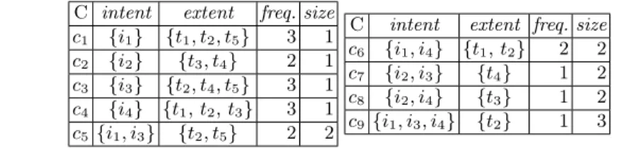
Table 1. Left: Example of transactional dataset withm= 5 transactions and n= 4
items. Right: SetF of formal concepts for this dataset.
i1 i2 i3 i4 t1 1 0 0 1 t2 1 0 1 1 t3 0 1 0 1 t4 0 1 1 0 t5 1 0 1 0
C intent extent freq. size
c1 {i1} {t1, t2, t5} 3 1
c2 {i2} {t3, t4} 2 1
c3 {i3} {t2, t4, t5} 3 1
c4 {i4} {t1,t2,t3} 3 1
c5 {i1, i3} {t2, t5} 2 2
C intent extent freq. size
c6 {i1, i4} {t1,t2} 2 2
c7 {i2, i3} {t4} 1 2
c8 {i2, i4} {t3} 1 2
c9 {i1, i3, i4} {t2} 1 3
The two objective functions that we consider are complementary and are related to the number of clusters: when maximizing concept sizes, optimal clus-terings have many clusters of small frequencies; when maximizing concept fre-quencies, optimal clusterings have very few clusters of small sizes. In Section5, we propose to compute the Pareto front of all non-dominated solutions, and we introduce and compare different ways for achieving this with our CP models.
2
Background on Conceptual Clustering
Formal Concepts. Formal Concept Analysis is a way of grouping together objects sharing a same set of attribute values [5]. In this paper, we use the transactional database terminology: objects are called transactions, and attribute values are calleditems. More formally, letT be a set ofmtransactions (numbered from 1 to
m),Ia set ofnitems (numbered from 1 ton), andR ⊆ T × I a binary relation that relates transactions to items: (t, i) ∈ R denotes the fact that transaction
t has item i. We note itemset(t) the set of items associated with t, i.e., ∀t ∈ T,itemset(t) ={i∈ I : (t, i)∈ R}. Given a set E, we noteP(E)the set of all its subsets, and#E its cardinality.
The intent of a subset T ⊆ T of transactions is the intersection of their itemsets, i.e., intent(T) =∩t∈Titemset(t). Theextentof a set I⊆ I of items is
the set of transactions whose itemsets contain I, i.e.,extent(I) ={t ∈ T :I⊆
itemset(t)}. These two operators induce a Galois connection betweenP(T)and
P(I),i.e.,∀T ⊆ T,∀I⊆ I, T ⊆extent(I)⇔I⊆intent(T). Aformal conceptis a couple(T, I)∈ P(T)× P(I)such thatT =extent(I)andI=intent(T). We note F the set of all formal concepts. The frequencyof a formal concept(T, I)
is the number of transactions,i.e.,f req(T, I) = #T, and itssizeis the number of items,i.e.,size(T, I) = #I.
For example, we display in table1a transactional dataset and its associated setF of formal concepts. The couple({t1, t2},{i1})is not a formal concept
be-causeintent({t1, t2}) ={i1, i4} 6={i1}andextent({i1}) ={t1, t2, t5} 6={t1, t2}.
Formal concepts and closed itemset mining. Formal concepts correspond to closed itemsets[18] and the set F may be computed by using algorithms dedi-cated to the enumeration of frequent closed itemsets, provided that the frequency threshold is set to 1. In particular, LCM [24] is able to extract all formal concepts
of F in linear time with respect to #F. As there is usually a huge number of closed itemsets, we may add constraints or optimization criteria to identify rele-vant concepts. For example, we may search for closed itemsets whose frequency is greater than some threshold and whose size is maximal. We may also combine several criteria, and search for the Pareto front of non dominated formal con-cepts (where a conceptc1is dominated by another conceptc2ifc2is at least as
good asc1 on all criteria but one, and strictly better on this last criterion). This
Pareto front is also called theskyline[2].
CP for itemset mining. Using CP to model and solve itemset search problems is a topic which has been widely explored during the last ten years [20,12,8,7]. Indeed, CP allows one to easily model various constraints on the searched item-sets, corresponding to application-dependent constraints for example. These con-straints are used to filter the search space during the mining process, and allow CP to be competitive with dedicated mining tools such as LCM. Most recently, [14] introduced a global constraint for extracting frequent closed itemsets. This global constraint enforces domain consistency in polynomial time, and it is quite competitive with LCM: if it is an order slower on basic queries, it is more effi-cient for complex queries where extra constraints are added. Also, [23] proposed to use CP to extract skyline patterns,i.e., non-dominated patterns according to several criteria: they use a dynamic approach, where constraints are added each time a new solution is found in order to forbid solutions dominated by it. Conceptual Clustering. Clustering is an unsupervised classification approach the goal of which is to group objects into homogeneous clusters. Conceptual clus-tering provides, in addition to clusters, a description of clusters by means of formal concepts: each cluster corresponds to a formal concept. More precisely, a conceptual clustering is a set of kformal conceptsC={(T1, I1), . . . ,(Tk, Ik)}
such that{T1, . . . , Tk} is a partition of the setT of transactions.
Different optimization criteria may be considered. In this article, we consider two classical criteria :minFreq, to maximize the minimal frequency of a cluster; and minSize, to maximize the minimal size of a cluster. For example, let us consider the set F of formal concepts displayed in table 1. Two examples of clusterings are P1 = {c1, c2} and P2 = {c1, c7, c8}. According to minFreq, the
best clustering isP1(as the minimal frequency is 2 forP1and 1 forP2). According
tominSize, both clusterings are equivalent as their minimal size is 1.
The numberkof clusters is an important parameter which has a great influ-ence on the size and the frequency of the clusters: small values forkfavor clusters with larger frequencies and smaller sizes, whereas large values favor clusters with smaller frequencies and larger sizes.
CP for conceptual clustering. Conceptual clustering is related to closed itemset mining, as each cluster corresponds to a closed itemset. However, the goal is no longer to find closed itemsets that satisfy some constraints or optimize some criteria, but to find a subset of closed itemsets which partitions the set of trans-actions and optimizes some criteria. Conceptual clustering is a special case of
k-pattern set mining, as introduced in [9]: the conceptual clustering problem is defined by combining a cover and a non-overlapping constraint, and a CP model based on boolean variables is proposed to solve this problem.
[3] describes a CP model for clustering problems where a dissimilarity mea-sure between objects is provided. In this case, the goal is to find a partition of the objects which satisfies some constraints and optimizes an objective function defined by means of this dissimilarity measure. This CP model has been ex-tended to conceptual clustering in [4]. Experimental results reported in [4] show that this model outperforms the binary model of [7]. This model assumes that the number of clusters is defined by a constant k. There is an integer variable
Gt for each transaction t ∈ T: Gt represents the cluster of t and its domain
is D(Gt) = [1, k]. Symmetries (due to the fact that cluster numbers may be
swapped) are broken by adding aprecede(G,[1, k])constraint [13]. Each cluster is enforced to have at least one transaction by the constraint: atLeast(1, G, k). For each clusterc∈[1, k], a set variableIntentc represents the intent of the set
of transactions inc,i.e., the intersection of their itemsets. Its domain is the set of all possible itemsets,i.e.,D(Intentc) =P(I). The extent constraint is expressed
by:∀c∈[1, k],∀t∈ T, Gt=c⇔Intentc⊆itemset(t). It is implemented thanks
to k×mreified constraints (withm= #T). The intent constraint is expressed by: ∀c ∈ [1, k], Intentc = ∩t∈T,Gt=citemset(t). It is implemented thanks to k constraints, and each of these k constraints needsnreified domain constraints to build the set of all transactions in cluster c, and a set element global con-straint to select the corresponding itemsets and intersect them. An objective variable is introduced. Depending on the optimization criterion, this variable is constrained to be equal either to the minimal cardinality of allIntentc variables
(minSize), or the minimal number of G variables assigned to a same cluster thanks toatLeast(obj, G, c)constraints (minFreq).
The model proposed in [4] assumes that the number of clusters is fixed to a constant valuek. It may easily be extended to the case where this number is not known, by introducing an integer variablek, whose domain is bounded between
2 andm−1. However, performance is degraded whenkis not fixed.
ILP for Conceptual Clustering. [17] proposes to compute conceptual clusterings by combining two exact techniques: in a first step, a dedicated closed itemset mining tool (i.e., LCM [24]) is used to compute the setF of all formal concepts and, in a second step, ILP is used to select a subset ofFthat is a partition of the set T of transactions and that optimizes some given criterion. More precisely, for each formal conceptf ∈ F, there is a binary variablexf such thatxf = 1iff
f is selected. The subset of selected formal concepts is constrained to define a partition ofT by posting the constraint:∀t∈ T,P
f∈Fatfxf = 1, whereatf = 1
if transactiontbelongs to the extension of conceptf, and 0 otherwise. Contrary to the CP approaches of [7,3], the number of clusters is not fixed and it is a variable k which is constrained to be equal to the number of selected concepts by posting the constraint: k = P
f∈Fxf. In [17], the goal is to maximize the
sum of the sizes of the selected concepts. Therefore, the objective function to maximize is:P
explicitly discussed in [17], we may easily extend this ILP model to maximize the minimal size (resp. frequency) of the selected concepts: we introduce a variable
vmin and enforce this variable to be smaller than or equal to the size (resp.
the frequency) of the selected concepts by adding the constraint∀t∈T, vmin≤
vfxf+M(1−xf), whereM is a positive constant greater than the largest possible
size (resp. frequency), andvf is the size (resp. frequency) of the conceptf.
3
New CP models
In this section, we introduce two new CP models for computing optimal concep-tual clusterings. The first model (described in Section 3.1) may be seen as an improvement of the CP model of [3]. The second model (described in Section 3.2) follows the two step approach of [17]: the first step is exactly the same; the second step uses CP to select formal concepts. These models are experimentally evaluated and compared with the approaches of [3] and [17] in Section4.
For both models, we do not assume that the number of clusters is fixed: k
is a variable whose domain is[kmin, kmax], wherekmin and kmax are two given
bounds such that2≤kmin≤kmax< m.
3.1 New full CP model
Like the CP model of [3], we useGcinteger variables to model clusters. However,
we associate theIntentset variables to transactions instead of associating them to clusters. This simplifies the propagation of the intent constraint. Another reason for associating Intent set variables to transactions instead of clusters is that, when k is strictly lower than kmax, each Intentc set variable such that
c > k should be empty. This would imply to use reification to compute the minimal intent size, as we must not consider Intentc variables such thatc > k
(otherwise, the minimal size would be equal to 0 wheneverk < kmax). Also, we
introduce new set variables to explicitly model extents and these set variables are associated with transactions to ease the computation of the minimal frequency. Finally, we introduce redundant set variables which model concept extents and are associated with clusters: these variables are used to add a redundant partition constraint which improves the solution process.
More formally, we use the following variables:
– an integer variablek(withD(k) = [kmin, kmax]), which represents the
num-ber of clusters;
– for each transactiont∈ T:
• an integer variable Gt(with D(Gt) = [1, kM ax]), which represents the
cluster oft;
• a set variableIntentt (withD(Intentt) =P(itemset(t))), which
repre-sents the set of items in the intent of the cluster oft;
• a set variableExtentt(withD(Extentt) =P(T)), which represents the
– for each clusterc∈[1, kmax], a set variableExtentClusterc (with
D(ExtentClusterc) =P(T)), which represents the set of transactions inc; – two integer variablesminF req(withD(minF req) = [1, m−1]) andminSize
(withD(minSize) = [1, n−1]), which represent the minimal frequency and size, respectively.
As proposed in [4,3], we break symmetries (due to the fact that clusters may be swapped) by posting the constraint:precede(G,[1, kmax]).
We relate extentt and extentClusterc variables by posting the constraint: ∀t ∈ T, Extent[t] =ExtentCluster[Gt], and we relateExtentClusterc and Gt
variables by posting the constraint
∀t∈ T,∀c∈[1, kmax], t∈ExtentClusterc⇔Gt=c
We add a redundant partition constraint that enforces extentto be a partition of T: partition(ExtentCluster,T). This constraint is redundant because each transaction is already enforced to belong to exactly one cluster by Gvariables. However, its propagation both reduces the search space and the CPU time.
We reifym(m−1)/2equality constraints betweenGvariables to ensure that two transactions are in a same cluster iff they have the same intent, and this intent is included in their itemsets:∀{t1, t2} ⊆ T
(Gt1 =Gt2)⇔(Intentt1 =Intentt2)⇔(Intentt1 ⊆itemSet(t2))
This constraint ensures the extent property as any transaction t1 such that
itemset(t1)⊇Intentt2 is constrained to be in the same cluster ast2. However,
this constraint only partially ensures the intent property: for each transactiont, it ensuresIntentt⊆ ∩t0∈T,G
t=Gt0itemset(t
0)whereas the intent property requires
that Intentt is equal to the itemset intersection. However, given any solution
that satisfies the constraint Intentt ⊆ ∩t0∈T,G
t=Gt0itemset(t
0), we can easily
transform it to ensure that it fully satisfies the intent property by adding to
Intenttevery item i ∈(∩t0∈T,G
t=Gt0itemset(t
0))\Intent
t. Hence, each time a
solution is found, for each clusterc, we compute its actual intent by intersecting the intersection of all its transaction itemsets. This ensures that each cluster actually is a formal concept, and therefore this ensures correction. Completeness is ensured by the fact that our constraint is a relaxation of the initial constraint. Finally, we compute the minimal size and frequency by posting the con-straints:minSize= mint∈T #IntenttandminF req= mint∈T #Extentt.
The search strategy depends on the objective function: if the goal is to max-imize minF req, then we first assignk to its lower values (as a smaller number of clusters usually leads to concepts with larger frequencies), whereas if the goal is to maximizeminSize, then we first assign k to its higher values (as a larger number of clusters usually leads to concepts with larger sizes).
3.2 New hybrid model
This model solves the problem in two steps as in [17]: in a first step, we extract the setF of all formal concepts with a dedicated tool (LCM), and in a second step we use CP to select the subset ofF forming an optimal clustering.
We have designed and compared several CP models for this second step. In particular, we have designed a model that associates a set variableExtentc with
each cluster c (such thatExtentc contains all transactions in the extent ofc),
and then post a partition global constraint on these variables to ensure that they form a partition of T. This model is always outperformed by the model described below.
Our CP model for the second step uses the following variables:
– an integer variablek(withD(k) = [kmin, kmax]), which represents the
num-ber of clusters (i.e., the number of selected concepts);
– a set variableP (with D(P) =P(F)), which represents the set of selected formal concepts that define an optimal clustering;
– for each transactiont∈ T, an integer variableConceptt(withD(Conceptt) = {f ∈ F |t∈extent(f)}), which represents the concept that containstin its extent (each transaction must belong to exactly one selected concept); – two integer variablesminF req(withD(minF req) = [1, m−1]) andminSize
(withD(minSize) = [1, n−1]), which represent the minimal frequency and size, respectively.
To ensure thatConceptt belongs to P, for each transactiont∈ T, we post the
constraint: ∀t∈ T, member(Conceptt, P).
To ensure that the selected concepts define a partition ofT, we ensure that each transactiontis contained in the extent of exactly one selected formal con-cept. To this aim, we compute, for each transaction t, the set CF(t)of all the concepts ofF that containtin their extent,i.e.,
∀t∈ T, CF(t) ={f ∈ F:t∈extent(f)}
and we ensure that the set variableP contains exactly one element ofCF(t)by posting the constraint:∀t∈ T,#(CF(t))∩P) = 1.
Finally, we compute the minimal size and frequency by posting the con-straints:minSize= mint∈T #intent(Ct)andminF req= mint∈T#extent(Ct).
The number of clusters of the solution is constrained in two different ways according to the objective function:
– If the goal is to maximize minF req, optimal solutions often have a small number of clusters and, in this case, we ensure thatkis equal to the number of distinct values contained inC by posting the constraint:nV alue(C, k). – If the goal is to maximizeminSize, optimal solutions often have a large
num-ber of clusters and, in this case, we ensure thatkis equal to the cardinality ofP by posting the constraint#P =k.
The search strategy also depends on the objective function. The idea is to first select concepts with large sizes (resp. frequency) when the goal is to maximize
minSize (resp.minF req). To this aim, we sort formal concepts by decreasing size (resp. frequency), and use this order as value ordering heuristic forCt. We
use a First failstrategy to select the variable with the smallest domain as next variable.
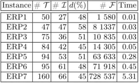
Table 2.Test instances: each row gives the number of transactions (#T), the number of items (#I), the density (d), the number of formal concepts (#F), and the CPU time (in seconds) spent by LCM to extract all formal concepts.
Instance #T #Id(%) #F Time ERP1 50 27 48 1 580 0.01 ERP2 47 47 58 8 1337 0.03 ERP3 75 36 51 10 835 0.03 ERP4 84 42 45 14 305 0.05 ERP5 94 53 51 63 633 0.28 ERP6 95 61 48 71 918 0.45 ERP7 160 66 45 728 537 5.31 Instance #T #Id(%) #F Time zoo 59 36 44 4 567 0.01 vote 341 48 34 227 031 0.54 tic-tac-toe 958 27 33 42 711 0.05 soybean 303 116 29 817 534 6.7
Furthermore, when the goal is to maximizeminF req, we use the ObjectiveS-trategy proposed by Choco [19], which performs a dichotomous branching over the domain ofminF req.
4
Experimental comparison for single objective problems
We compare our new models with the CP model of [3] and the ILP model of [17] for computing conceptual clusterings that optimize a single objective.
Experimental protocol. All experiments were conducted on Intel(R) Core(TM) i7-6700 with 3.40GHz of CPU and 65GB of RAM. The approach of [4] (called FullCP1) is implemented in Gecode v4.3. The approach of [17] (calledILP) uses LCM to extract formal concepts and Cplex v12.7 to solve the selection problem. Our CP model described in Section3.1(calledFullCP2) is implemented in Choco v.4.0.3 [19]. Our hybrid approach described in Section3.2(calledHybridCP) uses LCM v5.3 to extract formal concepts and Choco v.4.0.3 to solve the selection problem. We have limited the CPU time of each run to 1000 seconds.
Test instances. We consider four classical machine learning instances, coming from the UCI database: zoo, vote, tic-tac-toe, and soybean. We also introduce seven new instances (called ERPi, withi∈[1,7]) that have been extracted from our ERP database. Our ERP database contains 400 parameter settings: each setting corresponds to the customization of the ERP for a different client, and specifies the values of almost 450 different parameters. Each parameter can only take a finite number of values, and most of them are symbolic attributes. For each parameter/value couple, we have created a boolean item (set to 1 iff the parameter is assigned to the value in the setting). We have split this database into smaller ones by focusing on different groups of parameters, thus obtaining seven instances of various sizes3. All instances are described in Table 2.
3
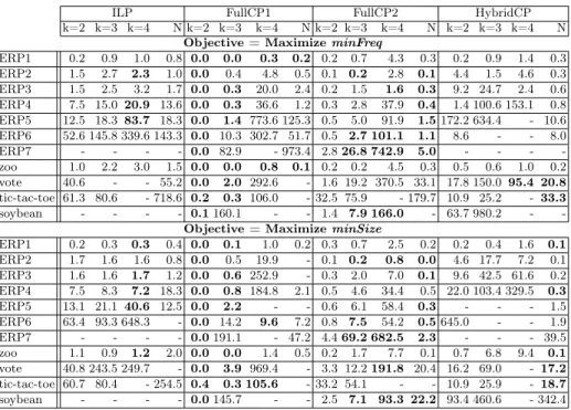
Table 3.Times when the goal is to optimizeminFreq(upper part) andminSize(lower part): each line gives the time of the four approaches whenk is fixed to 2, 3, and 4, respectively, and whenkis not fixed (N). ’-’ is reported when time exceeds 1000s.
ILP FullCP1 FullCP2 HybridCP
k=2 k=3 k=4 N k=2 k=3 k=4 N k=2 k=3 k=4 N k=2 k=3 k=4 N
Objective = MaximizeminFreq
ERP1 0.2 0.9 1.0 0.8 0.0 0.0 0.3 0.2 0.2 0.7 4.3 0.3 0.2 0.9 1.4 0.3 ERP2 1.5 2.7 2.3 1.0 0.0 0.4 4.8 0.5 0.1 0.2 2.8 0.1 4.4 1.5 4.6 0.3 ERP3 1.5 2.5 3.2 1.7 0.0 0.3 20.0 2.4 0.2 1.5 1.6 0.3 9.2 24.7 2.4 0.6 ERP4 7.5 15.0 20.9 13.6 0.0 0.3 36.6 1.2 0.3 2.8 37.9 0.4 1.4 100.6 153.1 0.8 ERP5 12.5 18.3 83.7 18.3 0.0 1.4 773.6 125.3 0.5 5.0 91.9 1.5172.2 634.4 - 10.6 ERP6 52.6 145.8 339.6 143.3 0.0 10.3 302.7 51.7 0.5 2.7 101.1 1.1 8.6 - - 8.0 ERP7 - - - - 0.0 82.9 - 973.4 2.826.8 742.9 5.0 - - - -zoo 1.0 2.2 3.0 1.5 0.0 0.0 0.8 0.1 0.2 0.2 4.5 0.3 0.5 0.6 1.0 0.2 vote 40.6 - - 55.2 0.0 2.0 292.6 - 1.6 19.2 370.5 33.1 17.8 150.0 95.4 20.8 tic-tac-toe 61.3 80.6 - 718.6 0.2 0.3 106.0 - 32.5 75.9 - 179.7 10.9 25.2 -33.3 soybean - - - - 0.1160.1 - - 1.4 7.9 166.0 - 63.7 980.2 -
-Objective = MaximizeminSize
ERP1 0.2 0.3 0.3 0.4 0.0 0.1 1.0 0.2 0.3 0.7 2.5 0.2 0.2 0.4 1.6 0.1 ERP2 1.7 1.6 1.6 0.8 0.0 0.5 19.9 - 0.1 0.2 0.8 0.0 4.6 17.7 7.2 0.1 ERP3 1.6 1.6 1.7 1.2 0.0 0.6 252.9 - 0.3 2.0 7.0 0.1 9.6 42.5 61.6 0.2 ERP4 7.5 8.3 7.2 18.3 0.0 0.8 184.8 2.1 0.5 4.6 34.4 0.5 22.0 103.4 329.5 0.3 ERP5 13.1 21.1 40.6 12.5 0.0 2.2 - - 0.6 6.1 58.4 0.3 - - - 1.5 ERP6 63.4 93.3 648.3 - 0.0 14.2 9.6 7.2 0.8 7.5 54.2 0.5645.0 - - 1.9 ERP7 - - - - 0.0191.1 - 47.2 4.469.2 682.5 2.3 - - - 39.5 zoo 1.1 0.9 1.2 2.0 0.0 0.0 1.4 0.5 0.2 1.7 7.7 0.1 0.7 6.8 9.4 0.1 vote 40.8 243.5 249.7 - 0.0 3.9 969.4 - 3.3 12.2191.8 20.4 16.2 69.0 -17.2 tic-tac-toe 60.7 80.4 - 254.5 0.4 0.3 105.6 - 33.2 54.1 - - 10.9 25.9 -18.7 soybean - - - - 0.0145.7 - - 2.5 7.1 93.3 22.2 93.4 460.6 - 342.4
Computation ofFwith LCM. Table2displays the time spent by LCM to extract all formal concepts, for each instance. This time is proportional with the size of
F, as the complexity of LCM is linear with respect to#F. CPU time is smaller than one second for all instances but two, and it is smaller than seven seconds for the instance that has the largest number of formal concepts (soybean). Comparison of scale-up properties of the different approaches. Table 3displays the times for computing optimal clusterings when the goal is to maximize min-Freq (upper part) orminSize (lower part). We report times when k is fixed to 2, 3, and 4, respectively, and then when k is not fixed (with kmin = 2 and
kmax =m−1). Times displayed for ILP and HybridCP both include the time
spent by LCM to extract all formal concepts.
For all approaches and all instances, time increases when increasingk from
2 to 4. FullCP1 and FullCP2 are more efficient when k = 2 than when k is not fixed, and they are more efficient when k is not fixed than when k = 4. HybridCP approach needs more time to solve the problem when k = 2 than when k is not fixed for all instances but three (vote, tic-tac-toe and soybean) whereas ILP approach needs more time only for the smallest ERP instances.
Whenk= 2, the best approach is FullCP1, which is able to solve all instances in less than 0.1 second (except tic-tac-toe). However, when increasingk from 2
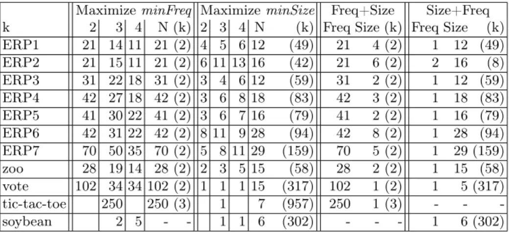
Table 4.Experimental comparison of frequencies, sizes, and number of clusters: each line displays the optimal values of minFreq and minSize when k is set to 2, 3, and 4, and when k is not fixed (N), followed by the value of k in the optimal solution (in brackets). Finally, it displays the optimal values of minFreq and minSize when maximizingminFreqand breaking ties withminSize(Freq+Size), and when maximizing
minSize and breaking ties withminFreq(Size+Freq). In this case, k is not fixed and its value in the optimal solution is displayed in brackets.
MaximizeminFreq MaximizeminSize Freq+Size Size+Freq k 2 3 4 N (k) 2 3 4 N (k) Freq Size (k) Freq Size (k) ERP1 21 14 11 21 (2) 4 5 6 12 (49) 21 4 (2) 1 12 (49) ERP2 21 15 11 21 (2) 6 11 13 16 (42) 21 6 (2) 2 16 (8) ERP3 31 22 18 31 (2) 3 4 6 12 (59) 31 2 (2) 1 12 (59) ERP4 42 27 18 42 (2) 3 6 8 18 (83) 42 3 (2) 1 18 (83) ERP5 41 30 22 41 (2) 3 6 7 16 (79) 41 2 (2) 1 16 (79) ERP6 42 31 22 42 (2) 8 11 9 28 (94) 42 8 (2) 1 28 (94) ERP7 70 50 35 70 (2) 5 8 11 29 (159) 70 5 (2) 1 29 (159) zoo 28 19 14 28 (2) 2 3 5 15 (58) 28 2 (2) 1 15 (58) vote 102 34 34 102 (2) 1 1 1 15 (317) 102 1 (2) 1 5 (317) tic-tac-toe 250 250 (3) 1 7 (957) 250 1 (3) - - -soybean 2 5 - - 1 1 6 (302) - - - 1 6 (302)
to 3, times of FullCP1 are strongly increased (up to 191 seconds for ERP7 with minSize) and FullCP1 is outperformed by FullCP2 for 8 instances. When further increasingkto 4, FullCP2 becomes the only approach able to solve all instances but tic-tac-toe, though ILP is able to solve 8 instances quicker.
Whenk is not fixed, the best performing approaches are fullCP2 (which is able to solve all instances but soybean for minFreq) and HybridCP (which is able to solve all instances forminSize).
Maximization of the sum of sizes. In [17], the objective function to maximize is the sum of the sizes of the selected concepts, and the proposed ILP model scales well for this objective: when k is not fixed, the time needed to find the optimal solution is 0.1, 0.4, 0.7, 1.7, 5.9, 14.0, and 183.2 for ERP1 to ERP7, respectively, and it is 0.3, 51.9, 32.0, and 120.0 for zoo, vote, tic-tac-toe, and soybean, respectively. Hence, ILP is more efficient for maximizing the sum of the sizes than for maximizingminSize. None of the CP models considered here scales well when the goal is to maximize the sum of the sizes, and they are far slower than ILP in this case: they usually very quickly find the optimal solution, but they are not efficient to prove optimality. However, we noticed that the optimal solutions found with the two criteria sum of sizes andminSizeare very similar (and often equal). Indeed, when maximizing the minimal size, we also tend to maximize the size of all concepts.
Comparison of frequencies, sizes, and number of clusters of optimal solutions. Table4displays the values ofminFreq,minSize, andkfor the optimal solutions
(tic-tac-toe does not have clusterings when k ∈ {2,4}, and soybean does not have clusterings when k = 2). It shows us that when k is fixed, the optimal values of minFreq and minSizeoften greatly vary when modifying the value of
k. For example, let us consider instance ERP4:minFreqdecreases from 42 to 27 and 18 (resp.minSize increases from 3 to 6 and 8) when k is increased from 2 to 3 and 4. From an applicative point of view, finding the relevant value for k
is not straightforward. When kis not fixed, we obtain extreme solutions: when the goal is to maximizeminFreq, there are only 2 clusters (except for tic-tac-toe, as there is no solution with k= 2), and when the goal is to maximize minSize, there arem−1clusters for all instances but 4 (ERP2, ERP3, ERP5 and vote), whereas for the remaining instances the value ofk is rather high.
Table4 also displays the values ofminFreq,minSize, andkwhen optimizing the two criteria in a lexicographic order and not fixingk. Let us call Freq+Size the solution that maximizes MinFreq while breaking ties with MinSize, and Size+Freq the solution that maximizes MinSize while breaking ties with Min-Freq. These solutions correspond to very different situations: for Freq+Size, k
is always equal to 2 (except for tic-tac-toe) andminSize is rather low (ranging between 1 and 8); for Size+Freq,kis equal tom−1for 6 instances, and rather large for the other instances, whileminFreqis always equal to 1, except for ERP2. From an applicative point of view, these solutions are not very interesting, and we need to find better compromises between size and frequency.
5
Multi-criteria optimization
As the two optimization criteria tend to produce extreme solutions which are not very meaningful for our application, we propose to compute the Pareto front of non dominated solutions. A clusteringC1is dominated by another clusteringC2
if the size and the frequency ofC1 are smaller than or equal to the size and the
frequency ofC2. Non dominated solutions correspond to different compromises
between the two criteria. The two extrema of the Pareto front are the solutions called Size+Freq and Freq+Size in the previous Section. In Section5.1, we ex-perimentally evaluate the efficiency of our two CP models for computing these extrema. Then, in Section5.2, we propose and compare different approaches for computing the whole Pareto front.
5.1 Computation of extrema solutions
Table5 displays the time spent by FullCP2 and HybridCP to compute the two extrema solutions of the Pareto front: Size+Freq is computed by first maximizing MinSize, fixing MinSize to its optimal value, and then maximizing MinFreq; Freq+Size is obtained by first maximizingMinFreq, fixingMinFreqto its optimal value, and then maximizingMinSize.
For Freq+Size, FullCP2 outperforms HybridCP on 6 instances and it is able to solve all instances except soybean while HybridCP is not able to solve ERP7, vote and soybean. However, for Size+Freq, FullCP2 is not able to solve 5 in-stances, while HybridCP is able to solve all instances but 2.
Table 5.Times needed to compute Size+Freq (left part) and Freq+Size (rightpart) for FullCP2 and HybridCP. For each solution, we first give the time needed to optimize the first criterion (1st), then the time needed to optimize the second criterion (2nd), and finally the total time (’-’ if total time exceeds 1000s).
Size+Freq Freq+Size
Instance FullCP2 HybridCP FullCP2 HybridCP 1st 2nd Total 1st 2nd Total 1st 2nd Total 1st 2nd Total ERP1 0.1 0.2 0.3 0.3 0.3 0.6 0.4 0.2 0.7 0.2 0.1 0.4 ERP2 - - - 0.1 0.3 0.4 0.2 0.1 0.3 0.3 0.3 0.6 ERP3 - - - 0.2 0.4 0.6 0.4 0.3 0.7 0.7 0.3 1.0 ERP4 0.4 6.9 7.3 0.6 1.5 2.1 0.5 0.5 1.0 0.8 0.1 0.9 ERP5 - - - 1.6 34.7 36.3 1.1 0.6 1.610.6 13.0 23.5 ERP6 0.5 1.4 1.9 4.0 94.2 98.2 1.6 0.7 2.3 8.0 59.8 67.9 ERP7 3.7 975.1978.8 - - - 6.3 2.9 9.2 - - -zoo 0.1 1.0 1.1 0.2 0.2 0.4 0.4 0.3 0.7 0.3 0.0 0.3 vote 20.0 6.2 26.2 18.3 648.7 667.0 26.5 13.5 40.0 - - -tic-tac-toe - - - 230.9 152.1 383.0 31.6 19.1 50.7 soybean - - - 325.0 342.1667.1 - - -
-5.2 Computation of the Pareto front
[3] describes a CP approach to compute non dominated bi-criteria clusterings by iteratively solving single criterion optimization problems while alternating between the two criteria. [6] describes a more dynamic CP approach to compute Pareto front: the idea is to search for all solutions, and dynamically add a con-straint each time a new solution is found to prevent the search from computing solutions that are dominated by it. This idea has been improved in [22,10]. We have experimentally compared these two approaches, and found that the dy-namic approach of [6] is more efficient than the static approach of [3] for our problem. Hence, we only consider this approach in this section. It proceeds as follows: we build an initial model as described in Section 3, and ask the solver to search for all solutions. Each time a solutionsol is found, we dynamically post the constraint(minFreq > f)∨(minSize > s)where f ands are the values of minFreq and minSizein sol, and go on the search for all solutions. The search stops when there is no more non-dominated solutions.
We have evaluated this dynamic approach with FullCP2 and HybridCP. FullCP2 is able to solve ERP1 in ten minutes, but fails to solve all other in-stances within a time limit of two hours. HybridCP is much more efficient, and is able to solve 6 instances within this time limit. Hence, we only consider Hy-bridCP in our experiments.
We have compared different variants of this dynamic approach. For all vari-ants, we use the two extrema solutions to reduce the search space in ana priori way. More precisely, letfFreq+SizeandsFreq+Size (resp.fSize+Freq andsSize+Freq) be the value ofminFreqandminSizein the solution Size+Freq (resp. Freq+Size).
We set the domain ofminFreqto [fSize+Freq+ 1, fFreq+Size−1]and the domain
ofminSizeto [sFreq+Size+ 1, sSize+Freq−1].
The first two variants correspond to the dynamic approach described below, with different search heuristics:freqseq (resp.sizeseq) uses the search heuristics
dedicated to the minFreq (resp.minSize) objective as described in Section 3.2. These two variants find complementary solutions at the beginning of the search process:freqseqfirst finds clusterings with large frequencies, whereassizeseqfirst
finds clusterings with large sizes. Hence, the variantfreqSizepar takes advantage
of this complementarity and launches the two variants in two parallel threads which communicate their solutions to update the non-dominated area: each time a solution is found by one thread, it dynamically adds constraints to filter the solutions dominated by this solution, and it also checks whether the other thread has found new solutions and dynamically adds constraints if ever.
The variantfreq+Dseq (resp. size+Dseq) decomposes the problem into two
subproblems by separating the domain ofminFreq(resp.minSize) in two equal parts. The two subproblems are solved sequentially. We first solve the sublem corresponding to the upper part of the domain, as no solution of this prob-lem can be dominated by a solution of the other subprobprob-lem. Then, we solve the second subproblem while preventing it from computing solutions that are dominated by the solutions of the first subproblem by adding constraints. The variants freq+Dpar and size+Dpar are similar tofreq+Dseq and size+Dseq: the
only difference is that they solve the two subproblems in two parallel threads. In this case, only one subproblem (the one with the upper part of the domain) communicates its solutions to the other thread.
Table6compares times of these different variants on 6 instances with a time limit of 2 hours (all other instances cannot be solved in less than 2 hours). For all instances, sizeseq is much more efficient than freqseq. Launching these two
approaches in two parallel threads does not pay off: freqSizepar is faster than sizeseqfor only two instances. This may come from the fact thatfreqseq is really
not efficient compared tosizeseq. Decomposing the problem into two subproblems
appears to be a better idea, even when solving the two subproblems sequentially, for thefreq-based variants:freq+Dseqis always much faster thanfreqseq. However, size+Dseq is faster than sizeseq for two instances only. Finally, solving the two
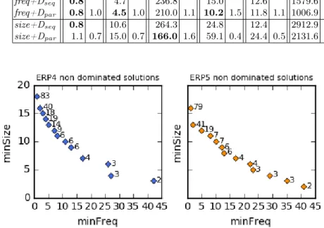
subproblems on two parallel threads always pays-off for the freq-based variants, whereas it degrades the solving time for 4 instances for thesize-based variants. Figure1 displays the Pareto fronts for ERP4 and ERP5.
6
Conclusion
We have introduced new CP models for computing optimal conceptual cluster-ings. These models are able to quickly find solutions that maximize either the minimal size or the minimal frequency, even when the number of clusters is not fixed. Computing the Pareto front for these two criteria is a more challenging problem, and our CP models are able to solve this problem in less than two hours for six instances only. Further work will mainly aim at improving this.
Table 6.Times to find all non-dominated solutions with different variants (’-’ if time exceeds 2 hours). parseq gives the speed-up between sequential and parallel variants (for
freqSizepar, we consider the best sequential time).
ERP1 zoo ERP4 ERP3 ERP2 ERP5 time parseq time parseq time seqpar time parseq time seqpar time parseq
freqseq 2.3 24.4 6048.7 145.7 41.7 5542.5 sizeseq 1.4 8.6 211.8 42.3 11.1 873.9 freqSizepar 1.4 1.0 7.0 1.2 216.5 1.0 36.0 1.2 12.7 0.9 1029.9 0.8 freq+Dseq 0.8 4.7 236.8 15.0 12.6 1579.6 freq+Dpar 0.8 1.0 4.5 1.0 210.0 1.1 10.2 1.5 11.8 1.1 1006.9 1.6 size+Dseq 0.8 10.6 264.3 24.8 12.4 2912.9 size+Dpar 1.1 0.7 15.0 0.7 166.0 1.6 59.1 0.4 24.4 0.5 2131.6 1.4
Fig. 1. Pareto front of ERP4 and ERP5: each point (x, y) corresponds to a non-dominated solution withx=minFreqandy=minSize. The numberkof clusters of the solution is displayed close to the point.
In particular, we plan to combine different decompositions to obtain more than two subproblems,e.g., both decompose the domains ofminFreqandminSize to obtain four subproblems that may be solved in four parallel threads. We also plan to evaluate scale-up properties of ILP for this problem, and combine ILP with CP if we observe complementary performance. Finally, we plan to evaluate the interest of combining our CP model with the propagation algorithm of [14].
Acknowledgments. We thank Jean-Guillaume Fages and Charles Prud’homme for enriching discussions on Choco, and authors of [4] for sending us their Gecode code.
References
1. M. Munir Ahmad and Ruben Pinedo Cuenca. Critical success factors for erp implementation in smes.Robot. Comput.-Integr. Manuf., 29(3):104–111, June 2013. 2. Stephan Börzsönyi, Donald Kossmann, and Konrad Stocker. The skyline operator. In Proceedings of the 17th IEEE International Conference on Data Engineering, pages 421–430, 2001.
3. Thi-Bich-Hanh Dao, Khanh-Chuong Duong, and Christel Vrain. Constrained Clus-tering by Constraint Programming. Artificial Intelligence, pages –, June 2015. 4. Thi-Bich-Hanh Dao, Willy Lesaint, and Christel Vrain. Clustering conceptuel et
relationnel en programmation par contraintes. InJFPC 2015, Bordeaux, France, June 2015.
5. Bernhard Ganter and Rudolf Wille.Formal Concept Analysis: Mathematical Foun-dations. Springer, 1997.
6. Marco Gavanelli. An algorithm for multi-criteria optimization in csps. In Proceed-ings of the 15th European Conference on Artificial Intelligence, ECAI’02, pages 136–140, Amsterdam, The Netherlands, The Netherlands, 2002. IOS Press. 7. Tias Guns. Declarative pattern mining using constraint programming.Constraints,
20(4):492–493, 2015.
8. Tias Guns, Siegfried Nijssen, and Luc De Raedt. Itemset mining: A constraint programming perspective. Artif. Intell., 175(12-13):1951–1983, 2011.
9. Tias Guns, Siegfried Nijssen, and Luc De Raedt. k-pattern set mining under constraints. IEEE Trans. Knowl. Data Eng., 25(2):402–418, 2013.
10. Renaud Hartert and Pierre Schaus. A support-based algorithm for the bi-objective pareto constraint. InProceedings of the Twenty-Eighth AAAI Conference on Ar-tificial Intelligence, AAAI’14, pages 2674–2679. AAAI Press, 2014.
11. L. Hossain. Enterprise Resource Planning: Global Opportunities and Challenges: Global Opportunities and Challenges. IRM Press, 2001.
12. Mehdi Khiari, Patrice Boizumault, and Bruno Crémilleux. Constraint program-ming for mining n-ary patterns. InPrinciples and Practice of Constraint Program-ming - CP 2010 - 16th International Conference, CP 2010, St. Andrews, Scotland, UK, September 6-10, 2010. Proceedings, pages 552–567, 2010.
13. Yat Chiu Law and Jimmy H. M. Lee.Global Constraints for Integer and Set Value Precedence, pages 362–376. Springer Berlin Heidelberg, 2004.
14. Nadjib Lazaar, Yahia Lebbah, Samir Loudni, Mehdi Maamar, Valentin Lemière, Christian Bessiere, and Patrice Boizumault. A global constraint for closed fre-quent pattern mining. In Principles and Practice of Constraint Programming -22nd International Conference, CP 2016, Toulouse, France, September 5-9, 2016, Proceedings, pages 333–349, 2016.
15. R.S. Michalski.Knowledge Acquisition Through Conceptual Clustering: A Theoret-ical Framework and an Algorithm for Partitioning Data Into Conjunctive Concepts. Report (University of Illinois at Urbana-Champaign. Dept. of Computer Science). Department of Computer Science, University of Illinois at Urbana-Champaign, 1980.
16. Jaideep Motwani, Ram Subramanian, and Pradeep Gopalakrishna. Critical factors for successful erp implementation: Exploratory findings from four case studies.
Comput. Ind., 56(6):529–544, August 2005.
17. Abdelkader Ouali, Samir Loudni, Yahia Lebbah, Patrice Boizumault, Albrecht Zimmermann, and Lakhdar Loukil. Efficiently finding conceptual clustering models with integer linear programming. InProceedings of the Twenty-Fifth International
Joint Conference on Artificial Intelligence, IJCAI 2016, New York, NY, USA, 9-15 July 2016, pages 647–654, 2016.
18. Nicolas Pasquier, Yves Bastide, Rafik Taouil, and Lotfi Lakhal. Discovering fre-quent closed itemsets for association rules. In Database Theory - ICDT ’99, 7th International Conference, pages 398–416, 1999.
19. Charles Prud’homme, Jean-Guillaume Fages, and Xavier Lorca. Choco Documen-tation. TASC, INRIA Rennes, LINA CNRS UMR 6241, COSLING S.A.S., 2016. 20. Luc De Raedt, Tias Guns, and Siegfried Nijssen. Constraint programming for
itemset mining. InProceedings of the 14th ACM SIGKDD International Conference on Knowledge Discovery and Data Mining, Las Vegas, Nevada, USA, August 24-27, 2008, pages 204–212, 2008.
21. Lionel Robert, Ashley R. Davis, and Alexander McLeod. Erp configuration: Does situation awareness impact team performance? 2011 44th Hawaii International Conference on System Sciences (HICSS 2011), 00(undefined):1–8, 2011.
22. Pierre Schaus and Renaud Hartert. Multi-Objective Large Neighborhood Search, pages 611–627. Springer Berlin Heidelberg, Berlin, Heidelberg, 2013.
23. Willy Ugarte, Patrice Boizumault, Bruno Crémilleux, Alban Lepailleur, Samir Loudni, Marc Plantevit, Chedy Raïssi, and Arnaud Soulet. Skypattern mining: From pattern condensed representations to dynamic constraint satisfaction prob-lems. Artif. Intell., 244:48–69, 2017.
24. Takeaki Uno, Tatsuya Asai, Yuzo Uchida, and Hiroki Arimura. An Efficient Al-gorithm for Enumerating Closed Patterns in Transaction Databases, pages 16–31. Springer Berlin Heidelberg, 2004.