Multi-objective optimized fuzzy-PID controllers for fourth order nonlinear systems

Full Length Article

Multi-objective optimized fuzzy-PID controllers for fourth order

nonlinear systems

M.J. Mahmoodabadi

*, H. Jahanshahi

Department of Mechanical Engineering, Sirjan University of Technology, Sirjan, Iran

A R T I C L E I N F O Article history:

Received 13 July 2015 Received in revised form 28 December 2015 Accepted 26 January 2016 Available online 27 February 2016

Keywords: Fuzzy-PID controller Multi-objective optimization Genetic algorithm Particle swarm optimization Ball–beam system Inverted pendulum system

A B S T R A C T

In this paper, the Multi-objective Genetic Algorithm (MOGA) is used to obtain the Pareto frontiers of con-flicting objective functions for the fuzzy-Proportional-Integral-Derivative (fuzzy-PID) controllers. The ball– beam and inverted pendulum fourth order nonlinear systems are regarded as nonlinear benchmarks. The considered objective functions for the ball–beam system are the distance error of the ball, the angle error of the beam, and the control effort. For the inverted pendulum system, the objective functions are the distance error of the cart, the angle error of the pendulum, and the control effort, which must be mini-mized simultaneously. The Pareto fronts are compared with those obtained by Multi-objective Particle Swarm Optimization (MOPSO). Four points are chosen from nondominated solutions of the obtained Pareto fronts based on the three conflicting objective functions and used for illustration of the state variables of the controlled systems. Obtained results elucidate the efficiency of the proposed controller in order to control nonlinear systems.

© 2016, Karabuk University. Publishing services by Elsevier B.V.

1. Introduction

Zadeh originally proposed the fuzzy logic and the fuzzy set theory [1,2]. Fuzzy systems are knowledge-based or rule-based systems formed via human knowledge and heuristics. They have been applied for a wide range of researching fields, such as control, communi-cation, medicine, management, business, psychology, etc. The most significant applications and studies about fuzzy systems have con-centrated on the control area[3–10]. The development of fuzzy-PID controllers for various engineering problems has been a major research activity in recent years. Duan et al. proposed an inherent saturation of the fuzzy-PID controller revealed due to the finite fuzzy rules[11]. Karasakal et al. applied fuzzy PID controllers based on an online tuning method and rule weighing in[12]. Boubertakh et al. proposed new auto-tuning fuzzy PD and PI controllers using reinforcement-learning algorithm for single-input single-output and two-input two-output systems[13]. In this way, the heuristic pa-rameters of fuzzy-PID controllers have to be determined via an appropriate approach. A very effective way to choose these param-eters is the use of evolutionary algorithms[14], such as the Genetic Algorithm (GA)[15]and particle swarm optimization (PSO)[16],

etc. In[17], a constrained optimization of a simple fuzzy-PID system was designed for the online improvement of PID control perfor-mance during productive control runs. Oh et al. developed a design methodology for a fuzzy PD cascade controller for a ball–beam system using particle swarm optimization (PSO)[18]. Mahmoodabadi et al. designed fuzzy controllers for nonlinear systems using MOPSO based on the Lorenz dominance method[19]. Sahib proposed a type of controller consisting of proportional, integral, derivative, and second order derivative terms optimized using the PSO algorithm for an automatic voltage regulator system[20].

In this paper, a novel optimal fuzzy-PID control strategy is pro-posed and implemented on two nonlinear benchmark systems. Governing equations for ball–beam and inverted pendulum systems transformed to the state-space forms. Two fuzzy inference engines are utilized. Due to having some different objective functions, MOGA and MOPSO are applied and three and two dimensional Pareto front figures are shown. The conflicting objective functions for ball–beam system are the distance error of the ball, the angle error of the beam, and the control effort. For inverted pendulum system, those are the distance error of the cart, the angle error of the pendulum, and the control effort. The simulation results corresponding to the optimum points demon-strate that the designed controller has the superior performance in comparison with reported results in published literature.

The rest of this paper is organized as follows.Section 2gives a brief description on the fuzzy-PID controller.Section 3presents the multi-objective optimization genetic algorithm. InSection 4, the * Corresponding author. Tel.:+98 34 423 36901; fax:+98 34 423 36900.

E-mail address:[email protected](M.J. Mahmoodabadi). Peer review under responsibility of Karabuk University.

http://dx.doi.org/10.1016/j.jestch.2016.01.010

2215-0986/© 2016, Karabuk University. Publishing services by Elsevier B.V.

Contents lists available atScienceDirect

Engineering Science and Technology,

an International Journal

j o u r n a l h o m e p a g e : h t t p : / / w w w. e l s e v i e r. c o m / l o c a t e / j e s t c h

Press: Karabuk University, Press Unit ISSN (Printed) : 1302-0056 ISSN (Online) : 2215-0986 ISSN (E-Mail) : 1308-2043

Available online at www.sciencedirect.com ScienceDirect

are recalled. Furthermore, their optimal fuzzy-PID controllers, simulation results and comparison studies to verify the capability of the proposed controller are shown in this section. Finally,Section 5concludes the paper.

2. Fuzzy-PID controller

The PID controller has a long history in the control engineering and is accepted in a lot of real applications due to the simple struc-ture. Hence, this controller is widely used still in so many industrial applications despite offering several new techniques. Consider a fourth order nonlinear system with Equation(1).

x_{= +}f1 b F1

θ

= +f2 b F2 (1)

wheref1,f2,b1, andb2are nonlinear functions andFis the control

input. The state-space formulation of the system can be written as Equation(2). x1=x2 x2=x3 x3= +f1 b F1 (2) x4=x5 x5=x6 x6= +f2 b F2

where x=

[

x x x x x x1, 2, 3, 4, 5, 6

]

= ⎡⎣∫x x x, , , ∫θ θ θ, ,⎤⎦is the state vector with desired value xd₌

[

x x x x x xd d d d d d

]

x x xd d d d d d

= ⎡⎣∫ ∫ ⎤⎦

1, 2, 3, 4, 5, 6 , , , θ θ θ, , . The PID controller with inputs e tx

( )

= −x xdand e tθ

( )

= −θ θd and

output Fpid

( )

t is commonly defined as Equation(3).

F K e t K e d K de t dt K e t K e d pid px x ix x t dx x p i =

( )+

( )

+

( )

+

( )

+

( )

∫

τ τ

τ

θ θ θ θ 0

ττ

θ θ 0 t d K de t dt

∫

+

( )

(3)

whereKp,Ki, andKdare the proportional, integral, and derivative gains, respectively. The adjustment and determination of these design parameters are key issues to design PID controllers. Hence, the fuzzy logic approach is applied to calculate the gains adaptively.

FFuzzy pid=K fˆix 1+K fˆpx 2+K fˆdx 3+K fˆiθ 4+K fˆpθ 5+K fˆdθ 6 (4)

whereFFuzzy pidis the fuzzy-PID control action. f ii, =1 2, ,…,6are the fuzzy variables with inputs_∫xdt x dx _∫ dt

dt ddt

, , , θ ,θ_and θ_{, respectively, and}

should be obtained by Single Input Fuzzy Inference Motor (SIFIM). Furthermore, in Equation(4), the variablesKˆix,Kˆpx,Kˆdx,Kˆiθ,KˆpθandKˆdθ

are calculated by Equation(5).

ˆ Kix=Kixb+KixrΔW1 ˆ Kx=Kxb+ ΔKxr W2 ˆ Kdx=Kdxb +KdxrΔW3 ˆ Kiθ=Kibθ+KirθΔW4 ˆ K Kb Kr W θ= θ+ Δθ 5

where ΔW ii, =1 2, ,…,6 are the fuzzy variables with inputs ∫xdt x dx ∫ dt

dt

d dt

, , , θ ,θ_and θ_{, respectively, and should be obtained by}

Preferrer Fuzzy Inference Motor (PFIM). Kixb,K Kxb, dxb,Kbiθ,KθbandKdbθare

the base variables and Kixr,K Kxr, dxr,Kirθ,KθrandKdrθare the regulation

variables. The base and regulation variables can be obtained by the try and error process. However, one of the best solutions to find these to have an optimal controller is the use of optimization approaches such as evolutionary methods, such as the genetic algorithm.

3. Optimization

The genetic algorithm is an approach for solving optimization problems based on biological evolution via modification of a pop-ulation of individual solutions, repeatedly. At each level, individuals are chosen randomly from the current population (as parents) then employed to produce the children for the next generation. In this paper, toolbox optimization of MATLAB (R2012a) with the follow-ing operators is implemented for optimal design of the fuzzy-PID controllers.

3.1. Population size

Increasing the population size enables the genetic algorithm to search more points and thereby obtain a better result. However, the larger the population size, the longer it takes for genetic algo-rithm to compute each generation.

3.2. Crossover options

Crossover options specify how the genetic algorithm combines two individuals, or parents, to form a crossover child for the next generation.

3.3. Crossover fraction

The crossover fraction specifies the fraction of each popula-tion, other than elite children, that is made up of crossover children. 3.4. Selection function

Selection options specify how the genetic algorithm chooses parents for the next generation.

3.5. Migration options

Migration options specify how individuals move between sub-populations. Migration occurs if you set population size to be a vector of length greater than 1. When migration occurs, the best individu-als from one subpopulation replace the worst individuindividu-als in another subpopulation. Individuals that migrate from one subpopulation to another are copied. They are not removed from the source subpopulation.

3.6. Stopping criteria options

Stopping criteria determine what causes the algorithm to terminate.

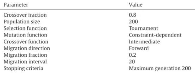
In this paper, the configuration of the genetic algorithm is set as the values given inTable 1.

Furthermore, the multi-objective optimization of the proposed fuzzy-PID controller would be done with respect to twelve design variables and three objective functions. The base values [Kixb,Kpxb,Kdxb, Kibθ,Kpbθ,Kdbθ] and regulation values [Kixr,Krpx,Kdxr,Kirθ,Kprθ,Kdrθ] are

the design variables. For ball–beam system, the distance error of the ball, the angle error of the beam and the control effort, and for inverted pendulum system, the distance error of the cart, the angle error of the pendulum and the control effort, are the objective func-tions. In other words, for both systems, the objective functions can be written as Equations(6) to (8).

Objective function 1₌

∫

x dt (6)

Objective function 2₌

∫

θ

dt (7)

Objective function 3₌

∫

F dt (8)

4. Optimal fuzzy-PID controller design

In this section, the optimal fuzzy-PID controller would be de-signed for the ball–beam and the inverted pendulum systems. 4.1. Ball–beam system

In the following, we consider the ball–beam system depicted in Fig. 1. The state vector is the system observable state vector x=

[

x x x x x x1, 2, 3, 4, 5, 6

]

= ⎡⎣∫x x x, , , ∫θ θ θ, ,⎤⎦, including, respectively, the integral of the ball position, the ball position, the ball velocity, in-tegral of the beam angle, the beam angle and the beam angular velocity. The dynamic equations of this system in the state-space form are expressed by Equation(9).

x1=x2 x2=x3 x3=B x x

[

2 62−gsin x

( )

5

]

x4=x5 x5=x6 x Mx x x gMx x J J Mx 6 2 3 6 2 5 1 2 22 2 = −

τ

_{+ +}− cos

( )

(9)

whereMis the ball mass,gis the gravity acceleration,J1is the ball

inertia moment, andJ2is the beam inertia moment. The

manipu-lated variableFis related with the torqueτby Equation(10).

τ

=2Mx x x2 3 6+gMx cosx2 5+

(

J1+ +J2 Mx F22

)

(10) whereFis the control input and F=FFuzzy pid. The system param-eters used for simulation are M=0.05kg, J1= ×2 10−6kgm2,

J2=0 02. kgm2, g=9 81. m_s2, andB=0.7143.

The initial and desired values are regarded as

x

( )

0 =

[

x1

( ) ( ) ( ) ( ) ( ) ( )

0,x2 0,x3 0,x4 0,x5 0,x6 0

]

=

[

0 0 5 0 0, . , , ,− °30, 00

]

and xd₌

[

x x x x x xd d d d d d

]

₌

[

]

1, 2, 3, 4, 5, 6 0 0 0 0 0 0, , , , , , respectively.

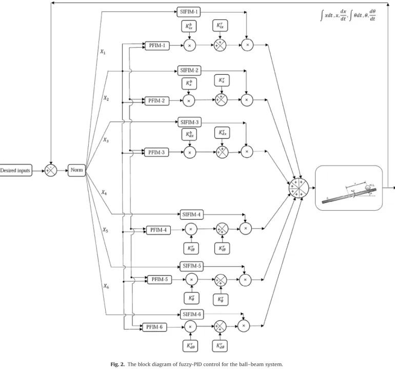
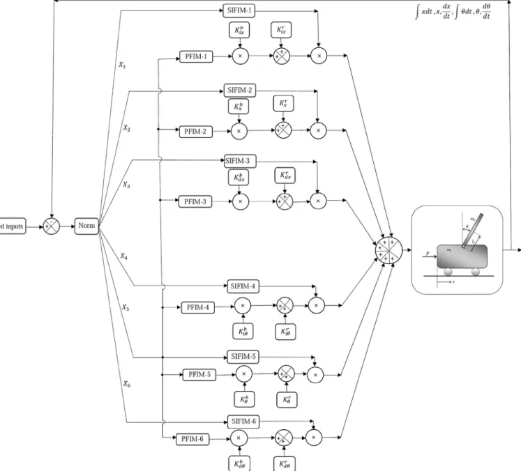
The block diagram for the stabilization control of the ball– beam system shown inFig. 2illustrates that each of the state variables _∫x x v, , ,_∫θ θ ω, , relevant to the ball–beam system is fed back and compared with its desired value. Since all of the desired values in the stabilization control are zeros, the variables are reversely in-putted into the Norm block for normalization of the state variables by their scaling factors. The scaling factors and the normalized form of the outputs are given inTable 2.

For ball–beam system, the Single Input Fuzzy Inference Motor (SIFIM) has only one input, and for each normalized variable (Norm block output) an SIFIM is defined. Since there are 6 Norm block output items, 6 SIFIMs would be created. For each input item X ii; =1 2, ,…,6, there is an SIFIM-i (f ii; =1 2, ,…,6). The Preferrer Fuzzy Inference Motor (PFIM) represents the control priority order of each Norm block output. The PFIM blocks for X ii; =1 2 3, , take the absolute values of the input itemsX2andX5as the antecedent

vari-ables, and the PFIM blocks for X ii; =4 5 6, , take the absolute value of the input itemX5as their antecedent variable. The membership

functions of SIFIMs are shown inTable 3andFig. 3, and their rules are mentioned inTables 4 and 5.

The output of f ii, =1 2, ,…,6for the ball and beam could be cal-culated using Equations(11)and(12).

Table 1

Genetic algorithm configuration parameters.

Parameter Value

Crossover fraction 0.8

Population size 200

Selection function Tournament

Mutation function Constraint-dependent

Crossover function Intermediate

Migration direction Forward

Migration fraction 0.2

Migration interval 20

Stopping criteria Maximum generation 200

Fig. 1. Structure of the ball–beam system.

Table 2

State variables and the associated scaling factors and normalized forms for the ball– beam system.

Variable Scaling factor Normalized form

xdt

∫

1 X1 x 1 X2 dx dt 1 X3 θdt

∫

1 X4 θ 45° X5 d dt θ 100°/s X6 Table 3

Membership functions of SIFIMs for the ball–beam system.

If Then Xi≤ −1 VBi=1 POi=0 ZBi=0 −1≤Xi≤0 VBi= −Xi POi=Xi+1 ZBi=0 0≤Xi≤1 VBi=0 POi= − +Xi 1 ZBi=Xi 1≤Xi VBi=0 POi=0 ZBi=1

f VB f PO f ZB f VB PO ZB i i= × + × + × + + = i i i i i i , , ˆ ˆ ˆ 1 2 3 1 2 3 (11) f VB f PO f ZB f VB PO ZB i i= × + × + × + + = i i i i i i , , ˆ ˆ ˆ 4 5 6 4 5 6 (12)

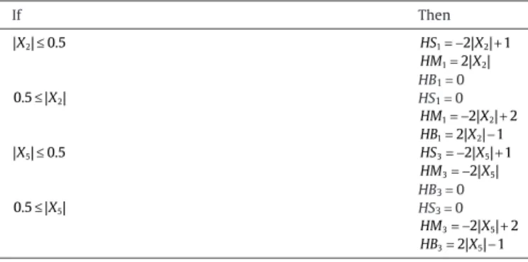
where variablesVB,PO, andZBare given inTable 3andFig. 3. The membership functions of PFIMs are illustrated inTable 6andFig. 4, and their rules are shown inTables 7 and 8.

Fig. 2.The block diagram of fuzzy-PID control for the ball–beam system.

Fig. 3. Membership functions of SIFIMs for the ball–beam system.

Table 4

Fuzzy rules of SIFIMs for the ball.

If X ii( =1 2 3, , ) Then

VBi ˆf1= −1

POi ˆf2=0

ZBi ˆf3=1

Table 5

Fuzzy rules of SIFIMs for the beam.

If X ii( =4 5 6, , ) Then

VBi fˆ4=1

POi fˆ5=0

The outputs of PFIMs for ball and beam,ΔW1,ΔW2,ΔW3, ΔW4,ΔW5andΔW6, can be calculated by Equations(13)and(14).

ΔWi=W ×HS ×HS +W ×HM ×HS +W ×HB ×HS +W ×HS ×HM +W ×HM ×HM 1 1 3 2 1 3 3 1 3 4 1 3 5 1 3++ × × × + × + × + × + × + × W HB HM HS HS HM HS HB HS HS HM HM HM HB HM 6 1 3 1 3 1 3 1 3 1 3 1 3 1 33 1 3 7 1 3 8 1 3 9 1 3 1 3 1 + × + × × + × × + × × + × + × HS HB W HS HB W HM HB W HB HB HM HB HB H … B B3 i 1 2 3 ; ₌ , , ΔW W HS W HM W HB HS HM HB i i= × + × + × + + = 10 3 11 3 12 3 3 3 3 4 5 6 ; , , (14) (13)

After calculation offiand ΔW ii; =1 2, ,…,6, it is possible to define the fuzzy-PID controller via Equation(4).

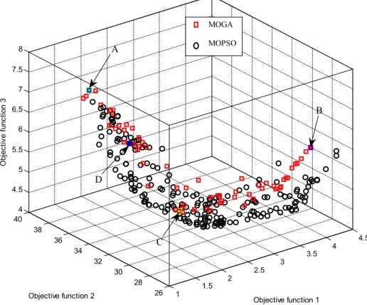
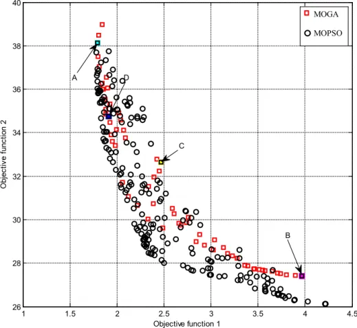
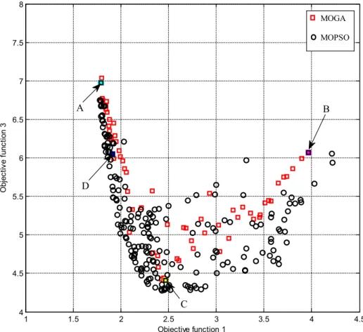
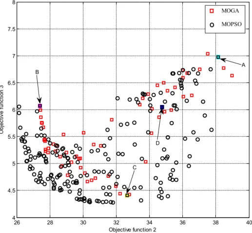
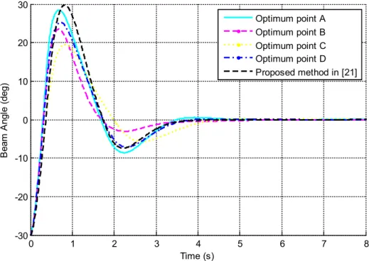
In the following, the multi-objective optimization of the pro-posed fuzzy-PID controller would be done by MOGA and MOPSO [19](with the same settings) with respect to the base and regula-tion parameters as design variables, and three objective funcregula-tions as the distance error of the ball, the angle error of the beam and the control effort. The optimum points of the objective functions are illustrated inFigs. 5–8. Points A, B and C are the best points for objectives 1, 2 and 3, respectively, and point D is a trade-off point. The time responses of the ball position, beam angle and control input for these optimum points are depicted inFigs. 9–11.

Although the complete stabilization occurs and all the state vari-ables converge to zero, by comparison of method proposed by Yi et al.[21]and this work, the superiority of this work from view-points of distance and angle error is obvious. In[21], as shown in Figs. 9 and 10, the ball position and beam angle reached the final state almost at 6 and 5.5 seconds, respectively, while this work can achieve almost 3 seconds for the ball position, 3.8 seconds for the beam angle and the maximum absolute of the control input is about 28.7 (point D). The values of design variables relative to point D and objective functions relative to points A, B, C, and D are given in Tables 9 and 10, respectively.

Table 6

Membership functions of PFIM for the ball–beam system.

If Then X2≤0 5. HS1= −2X2+1 HM1=2X2 HB1=0 0 5. ≤X2 HS1=0 HM1= −2X2+2 HB1=2X2−1 X5≤0 5. HS3= −2X5+1 HM3= −2X5 HB3=0 0 5. ≤X5 HS3=0 HM3= −2X5+2 HB3=2X5−1

Fig. 4. Membership functions of PFIM for the ball–beam system.

Table 7

Rules of PFIMs for the ball.

If Then X2 HS1 W1=0 X5 HS3 X2 HM1 W2=0.5 X5 HS3 X2 HB1 W3=1 X5 HS3 X2 HS1 W4=0 X5 HM3 X2 HM1 W5=0 X5 HM3 X2 HB1 W6=0.5 X5 HM3 X2 HS1 W7=0 X5 HB3 X2 HM1 W8=0 X5 HB3 X2 HB1 W9=0 X5 HB3 Table 8

Fuzzy rules of PFIM for the beam.

If Then

X5 HS3 W10=0

X5 HM3 W11=0 5.

X5 HB3 W12=1

Table 9

Design variables of optimum point D for fuzzy-PID control of the ball–beam system.

Design variable Value

Kixb 2.45 Kxb 6.98 Kdxb 7.75 Kibθ 17.40 Kb θ 32.09 Kdbθ 18.59 Kixr 1.24 Kxr 7.07 Kdxr 4.86 Kirθ 5.79 Kr θ 9.22 Kdrθ 8.71 Table 10

Objective functions of points A, B, C, and D for fuzzy-PID control of the ball–beam system. Point Value A Objective function 1=1.79 Objective function 2=38.13 Objective function 3=6.98 B Objective function 1=3.97 Objective function 2=27.40 Objective function 3=6.07 C Objective function 1=2.47 Objective function 2=32.65 Objective function 3=4.41 D Objective function 1=1.91 Objective function 2=34.75 Objective function 3=6.04

4.2. Inverted pendulum system

In the following, we consider the inverted pendulum system de-picted inFig. 12. x=

[

x x x x x x1, 2, 3, 4, 5, 6

]

= ⎡⎣∫x x x, , , ∫θ θ θ, ,⎤⎦, including, respectively, integral of the cart position, the cart position, the cart velocity, integral of the pendulum angle, the pendulum angle and the pendulum angular velocity. The dynamic equations of this system in the state-space form are expressed by Equation(15).

x1=x2 x2=x3 x F m l x x m gsin x x m m m cos p p p c p p 3 62 5 5 5 2 4 3 4 3 =

[

+

( )

]

−

( )

( )

+

(

)

− sin cos x x5

( )

x4=x5 x5=x6 x m m gsin x F m l x x x m m m c c p p p c p p 6 5 62 5 5 4 3 =

(

+

)

( )− +

[

( )

]

( )

+

(

)

− sin cos o os x lp 2 5

( )

⎡ ⎣⎢ ⎤⎦⎥ (15)

wheremcis the mass of the cart,mpis the mass of the pendulum, g is the gravity acceleration, and F is the control input and

F=11×FFuzzy pid.lp is the length from the center of the pendulum

to the pivot and equals to the half-length of the pendulum.

For simulation, the following specifications are used

mc=1kg m, p=0 1. kg l, p=0 5. m and g, =9 8. _sm2.

The initial and desired conditions are

x

( )

0 =

[

x1

( ) ( ) ( ) ( ) ( ) ( )

0,x2 0,x3 0,x4 0,x50,x6 0

]

=

[

0 2 0 0 0 0, , , , ,

]

and

xd₌

[

x x x x x xd d d d d d

]

₌

[

]

1, 2, 3, 4, 5, 6 0 0 0 0 0 0, , , , , , respectively. The block

diagram for the stabilization control of the inverted pendulum system illustrated in Fig. 13 shows that each of the state variables ∫x x v, , ,∫θ θ ω, , relevant to inverted pendulum system is fed back and compared with its desired value. Since all of the desired values in the stabilization control are zero, the variables are directly in-putted into the Norm block. The normalization of the state variables based on their scaling factors and creating input items X X X X X X1, 2, 3, 4, 5, 6 from ∫x x v, , ,∫θ θ ω, , , respectively, is done by the Norm block. The scaling factors and the normalized form of the Norm block outputs are given inTable 11.

Here, similar to fuzzy-PID control of the ball–beam system, two fuzzy inference engines SIFIM and PFIM are utilized. Each input item X ii; =1 2, ,…,6 is guided to the SIFIM-i, and f ii; =1 2, ,…,6are its output corresponding to the input itemXi. PFIM represents the control priority order of each Norm block output. All of the PFIM blocks take the absolute value of the input itemX5as their

ante-cedent variable. The membership functions of SIFIMs are depicted inTable 12andFig. 14. The rules of the PFIMs are given inTables 13 and 14. 1 1.5 2 2.5 3 3.5 4 4.5 26 28 30 32 34 36 38 40 4 4.5 5 5.5 6 6.5 7 7.5 8 Objective function 1 Objective function 2 O b je c ti v e fu n c ti o n 3

A

B

MOGA MOPSO

C

D

Fig. 5. Three-dimensional Pareto fronts of objective functions 1, 2 and 3 for the ball–beam system.

Table 11

Scaling factors and normalized forms of the state variables for the inverted pendu-lum system.

Variable Scaling factor Normalized form

xdt

∫

1 X1 x 2.4m X2 dx dt 1 X3 θdt

∫

1 X4 θ 30° X5 d dt θ 100°/s X6

The output of SIFIM-i (fi) for the cart and pendulum is calcu-lated by Equations(16)and(17), respectively.

f VB f PO f ZB f VB PO ZB i i= × + × + × + + = i i i i i i ; , , ˆ ˆ ˆ 1 2 3 1 2 3 (16) f VB f PO f ZB f VB PO ZB i i= × + × + × + + = i i i i i i ; , , ˆ ˆ ˆ 4 5 6 4 5 6 (17)

The membership functions of PFIMs are shown inTable 15and Fig. 15. The rules of the PFIMs are given inTables 16 and 17.

The outputs of PFIMs for ball and beam, ΔW1, ΔW2, ΔW3, ΔW4,

ΔW5and ΔW6, can be calculated by Equations(18)and(19).

ΔW W HS W HM W HB HS HM HB i i= × + × + × + + = 1 1 2 1 3 1 1 1 1 1 2 3 ; , , (18) 1 1.5 2 2.5 3 3.5 4 4.5 26 28 30 32 34 36 38 40 Objective function 1 O b je c ti v e f u nc ti on 2 D C B A MOGA MOPSO

Fig. 6.Pareto fronts of objective functions 1 and 2 for the ball–beam system.

Table 12

Membership functions of SIFIMs for the inverted pendulum system.

If Then Xi≤ −1 VBi=1 POi=0 ZBi=0 −1≤Xi≤0 VBi= −Xi POi=Xi+1 ZBi=0 0≤Xi≤1 VBi=0 POi= − +Xi 1 ZBi=Xi 1≤Xi VBi=0 POi=0 ZBi=1 Table 13

Fuzzy rules of SIFIMs for the cart.

If X ii(=1 2 3, , ) Then

VBi fˆ1= −1

POi fˆ2=0

ZBi fˆ3=1

Table 14

Fuzzy rules of SIFIMs for the pendulum.

If X ii(=1 2 3, , ) Then

VBi ˆf4= −1

POi ˆf5=0

ZBi ˆf6=1

Table 15

Membership functions of PFIM for inverted pendulum system.

If Then X2≤0 5. HS1= −2X2+1 HM1=2X2 HB1=0 0 5. ≤X2 HS1=0 HM1= −2X2+2 HB1=2X2−1

ΔW W HS W HM W HB HS HM HB i i= × + × + × + + = 4 1 5 1 6 1 1 1 1 4 5 6 ; , , (19)

where variablesHS1,HM1, andHB1are given inTable 15andFig. 15.

After calculation offiand ΔWi, it is possible to define the fuzzy-PID controller based on Equation(4).

The Pareto fronts obtained via the multi-objective genetic algo-rithm and particle swarm optimization[19](with the similar configurations) are given inFigs. 16–19. Points A, B, and C are the best points of objectives 1, 2, and 3, respectively, and point D is se-lected as a trade-off optimum point. Trade-off is the best point that is obtained by substituting base variables and regulation variables of all the optimal points achieved of optimization via genetic al-gorithm and acquiring the best condition according to settling time

and overshoot. The time responses of cart position, pendulum angular and derive force for the optimum points are illustrated in Figs. 20–22.

It is observable fromFigs. 20–22 that all the state variables converge to zero and complete stabilization occurs. Moreover, the superiority of this work in comparison with proposed approach in[22]is obvious. In[22], the cart position and pendu-lum angle reached the final state almost in 7.2 and 7.5 seconds, respectively, while this work can achieve almost 3 seconds for the ball position and 4 seconds for the beam angle and the maximum absolute of the control input is about 8.02 (Point D). The values of design variables relative to point D and objective functions rela-tive to points A, B, C, and D are given in Tables 18 and 19, respectively. 1 1.5 2 2.5 3 3.5 4 4.5 4 4.5 5 5.5 6 6.5 7 7.5 Objective function 1 O b je c tiv e f u n c ti o n 3

A

D

B

C

MOGA MOPSO

Fig. 7. Pareto fronts of objective functions 1 and 3 for the ball–beam system.

Table 16

Fuzzy rules of PFIMs for the cart.

If Then

X5 HS1 W1=1

X5 HM1 W2=0.5

X5 HB1 W3=0

Table 17

Fuzzy rules of PFIM for the beam.

If Then

X5 HS1 W4=0

X5 HM1 W5=0.5

X5 HB1 W6=1

Table 18

Design variables of optimum point D for fuzzy-PID control of the inverted pendu-lum system.

Design variable Value

Kixb 0.029 Kxb 0.583 Kdxb 0.110 Kibθ 2.88 Kb θ 2.61 Kdbθ 1.92 Kixr −0.030 Kxr 0.291 Kdxr 0.152 Kirθ 3.79 Kr θ −1.50 Kdrθ 5.00

26 28 30 32 34 36 38 40 4 4.5 5 5.5 6 6.5 7 7.5 8 Objective function 2 O b je c tiv e f u n c tio n 3 B A C D MOGA MOPSO

Fig. 8.Pareto fronts of objective functions 2 and 3 for the ball–beam system.

0

1

2

3

4

5

6

7

8

-0.2

0

0.2

0.4

0.6

0.8

1

1.2

1.4

Time (s)

Ba

ll Po

s

iti

o

n

(

m

)

Optimum point A

Optimum point B

Optimum point C

Optimum point D

Proposed method in [21]

0

1

2

3

4

5

6

7

8

-30

-20

-10

0

10

20

Time (s)

Be

a

m

An

g

le

(

d

e

g

)

Optimum point A

Optimum point B

Optimum point C

Optimum point D

Proposed method in [21]

Fig. 10.Time response of the beam angle for the ball–beam system.

0 1 2 3 4 5 6 7 8 -20 -15 -10 -5 0 5 10 15 20 25 30 Time (s) Co n tro l I n p u t Optimum point A Optimum point B Optimum point C Optimum point D Proposed method in [21]

Fig. 12. Structure of the inverted pendulum system.

Fig. 13. Block diagram of fuzzy-PID control for the inverted pendulum system.

In this work, multi-objective optimization algorithms, i.e. MOGA and MOPSO, were successfully used to optimum design the fuzzy-PID controllers for the ball–beam and inverted pendulum systems. An integral term was augmented to the state variables in order to eliminate the steady state errors and decrease the rising time. The conflicting objective functions for the ball–beam system were

Fig. 15. Membership functions of PFIM for the inverted pendulum system.

0 5 10 15 20 0 5 10 15 20 25 0 2 4 6 8 10 12 14 Objective function 1 Objective function 2 O bje ctiv e f un ctio n 3 C _B D A MOGA MOPSO

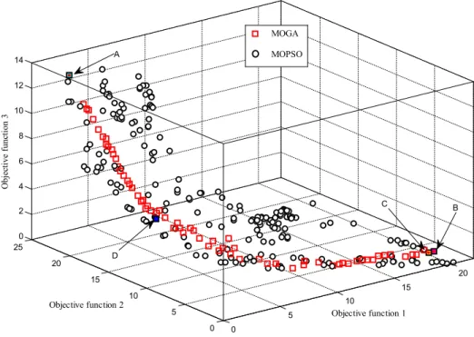
Fig. 16. Three-dimensional Pareto fronts of objective functions 1, 2 and 3 for the inverted pendulum system.

0 2 4 6 8 10 12 14 16 18 20 22 0 5 10 15 20 25 Objective function 1 Ob je c ti v e f u n c ti o n 2 A D C B MOGA MOPSO

0 2 4 6 8 10 12 14 16 18 20 22 0 2 4 6 8 10 12 14 Objective function 1 O b je c ti v e f u nc ti on 3 A B D C MOGA MOPSO

Fig. 18.Pareto fronts of objective functions 1 and 3 for the inverted pendulum system.

0 5 10 15 20 25 0 2 4 6 8 10 12 14 Objective function 2 O b je c ti v e f u nc ti on 3 C B A D MOGA MOPSO

0 1 2 3 4 5 6 7 8 -0.5 0 0.5 1 1.5 2 Time (s) Ca rt P o s it io n (m ) Optimum Point A Optimum Point B Optimum Point C Optimum Point D Proposed Method in [22]

Fig. 20.Time response of the cart position for the inverted pendulum system.

0 1 2 3 4 5 6 7 8 9 10 -15 -10 -5 0 5 10 15 Time (s) P e ndul um A n gl e ( d eg) Optimum Point A Optimum Point B Optimum Point C Optimum Point D Proposed Method in [22]

Fig. 21. Time response of the pendulum angle for the inverted pendulum system.

0 1 2 3 4 5 6 7 8 -10 -5 0 5 10 15 20 Time (s) C o nt ro l I n put Optimum Point A Optimum Point B Optimum Point C Optimum Point D Proposed Method in [22]

considered as the distance error of the ball, the angle error of the beam, and the control effort. The conflicting objective functions for the inverted pendulum system were considered as the distance error of the cart, the angle error of the pendulum, and the control effort. The reported results demonstrated that the proposed methodolo-gy can effectively control the nonlinear systems.

References

[1] L.A. Zadeh, Fuzzy algorithms, Inform. Contr. 12 (1968) 94–102.

[2] L.A. Zadeh, Outline of a new approach to the analysis of complex systems and decision processes, IEEE Trans. Syst. Man Cybern. 3 (1) (1973) 28–44.

[3] H. Nasser, E.H. Kiefer-Kamal, H. Hu, S. Belouettar, E. Barkanov, Active vibration damping of composite structures using a nonlinear fuzzy controller, Compos. Struct. 94 (4) (2012) 1385–1390.

[4] P. Li, F.J. Jin, Adaptive fuzzy control for unknown nonlinear systems with perturbed dead-zone inputs, Acta Automat. Sinica 36 (4) (2010) 573– 579.

[5] M. Marinaki, Y. Marinakis, G.E. Stavroulakis, Fuzzy control optimized by PSO for vibration suppression of beams, Control Eng. Pract. 18 (6) (2010) 618–629.

[6] D. Wang, X. Lin, Y. Zhang, Fuzzy logic control for a parallel hybrid hydraulic excavator using genetic algorithm, Automat. Constr. 20 (5) (2011) 581–587.

[7] R.E. Precup, M.B. Ra˘dac, M.L. Tomescu, E.M. Petriu, S. Preitl, Stable and convergent iterative feedback tuning of fuzzy controllers for discrete-time SISO systems, Expert Syst. Appl. 40 (1) (2013) 188–199.

[8] S.W. Tong, G.P. Liu, Real-time simplified variable domain fuzzy control of PEM fuel cell flow systems, Eur. J. Control 14 (3) (2008) 223–233.

[9] J.N. Lygouras, P.N. Botsaris, J. Vourvoulakis, V. Kodogiannis, Fuzzy logic controller implementation for a solar air-conditioning system, Appl. Energy 84 (12) (2007) 1305–1318.

[10] U. Zuperl, F. Cus, M. Milfelner, Fuzzy control strategy for an adaptive force control in end-milling, J. Mater. Process. Technol. 164–165 (2005) 1472–1478.

[11] X.G. Duan, H.X. Li, H. Deng, Robustness of fuzzy PID controller due to its inherent saturation, J. Process Contr. 22 (2) (2012) 470–476.

[12] O. Karasakal, M. Guzelkaya, I. Eksin, Online tuning of fuzzy PID controllers via rule weighing based on normalized acceleration, Eng. Appl. Artif. Intell. 26 (1) (2013) 184–197.

[13] H. Boubertakh, M. Tadjine, P.Y. Glorennec, Tuning fuzzy PD and PI controllers using reinforcement learning, ISA Trans. 49 (4) (2010) 543–551.

[14] R.E. Precup, R.C. David, E.M. Petriu, M.-B. Ra˘dac, S. Preitl, J. Fodor, Evolutionary optimization-based tuning of low-cost fuzzy controllers for servo systems, Knowl.-Based Syst. 38 (2013) 74–84.

[15] E. Sanchez, T. Shibata, L.A. Zadeh, Genetic Algorithms and Fuzzy Logic Systems, World Scientific, River Edge, NJ, 1997.

[16] J. Kennedy, R.C. Eberhart, Particle swarm optimization, in: Proceedings of the IEEE International Conference on Neural Networks, vol. 4, Perth, Australia, 1995, pp. 1942–1948.

[17] S.E. Mansour, G.C. Kember, R. Dubay, Online optimization of fuzzy-PID control of a thermal process, ISA Trans. 44 (2) (2005) 305–314.

[18] S.K. Oh, H.J. Jang, W. Pedrycz, Optimized fuzzy PD cascade controller: a comparative analysis and design, Simul. Model. Pract. Theory 19 (1) (2011) 181–195.

[19] M.J. Mahmoodabadi, M.B. Salahshoor Mottaghi, A. Mahmodinejad, Optimum design of fuzzy controllers for nonlinear systems using multi-objective particle swarm optimization, J. Vib. Control 22 (3) (2016) 769–783.

[20] M. Sahib, A novel optimal PID plus second order derivative controller for AVR system, Eng. Sci. Technol. Int. J. 18 (2015) 194–206.

[21] J. Yi, N. Yubazaki, K. Hirota, Stabilization control of ball and beam systems, in: IEEE/IFSA World Congress and 20th NAFIPS International Conference, Jul 25–Jul 28, vol. 4, Vancouver, BC, Canada, 2001, pp. 2229–2234.

[22] J. Yi, N. Yubazaki, Stabilization fuzzy control of inverted pendulum systems, Artif. Intell. Eng. 14 (2000) 153–163.

Table 19

Objective functions of points A, B, C, and D for fuzzy-PID control of the inverted pen-dulum system. Point Value A Objective function 1=2.32 Objective function 2=23.52 Objective function 3=12.89 B Objective function 1=19.41 Objective function 2=1.32 Objective function 3=0.79 C Objective function 1=19.18 Objective function 2=1.60 Objective function 3=0.64 D Objective function 1=3.18 Objective function 2=13.47 Objective function 3=3.90