Application of Basic Excel Programming to Linear Muskingum Model for Open Channel Routing

Application of Basic Excel Programming to Linear Muskingum

Model for Open Channel Routing

Martins Olalekan Oyekanmi* Kamar Taiwo Oladepo

Department of Civil Engineering, Obafemi Awolowo University, Ile-Ife, Nigeria Abstract

Flood routing as the process of determining the reservoir stage, storage volume of the outflow hydrograph corresponding to a known hydrograph of inflow. It is viable technique for determining the flood hydrograph at a section of a river by utilizing the flow data at one or more upstream sections. It can be hydraulic and hydrologic. Some hydrological routing techniques include Muskingum method, Muskingum-Cunge method, Lag method and Kalinin-Milyukov method while many sophisticated computer programs like Matlab had been deployed for river routing.Muskingum Method for stream routing was considered by using spreadsheet for. Coefficients were determine using various hydrologic data and formula for the Muskingum method. A popular data with other three data sets were considered in a linear model. The value of k and x was calculated using the basics of Microsoft Excel cell programming. Analysis of variance (One- way) was performed to detect any significant difference in the methods compared with other study without basics of excel.The result shows no significant difference with the values computed in this present study, limitations of Muskingum method were highlighted and further research the subject is recommended.

Keywords: Flood routing, hydrograph, Muskingum method, hydraulic, hydrologic, 1.0 INTRODUCTION

1.1 The Origin of Muskingum Method

The Muskingum method for flood routing was developed for the Muskingum Conservancy district (Ohio) flood control study in the 1930s and is one of the most popular methods of hydrological routing for drainage channels with all types of rivers and streams (Elbashir, 2011). The design of flood protection schemes in the Muskingum River Basin, Ohio, USA brought about this method of flow routing. Inflow and outflow is complex in a natural channel therefore, wedge and prism storage occurs in natural channels. Chin (2000) explained prism storage as the volume of a constant cross-section that corresponds to uniform flow in a prismatic channel. With the movement of flow, wedge storage is generated.

1.2 Open Flow in Rivers

Flow in open river channels especially natural channels like can be majorly unsteady, non-uniform and turbulent. These could also be sub-critical, critical and super-critical according to the Froude’s number. Therefore the Froude’s number is important parameter for analyzing open channel flow.

1.3 Equations Governing Open Channel Flow

The two most widely used formulas for solving open channel flow was given an Irish engineer Robert Manning and his engineering French colleague, Anthonie Chezy. The formulated what is known Mannings and Chezy’s formula. Manning’s Formula = (1.1) = = (1.2) = (1.3)

The roughness coefficient (n) for the Manning equation indicates the resistance of the channel bottom to flowing water (Elbashir, 2011).

The wetted perimeter (P) is described as the distance along the channel bottom below the water surface (Boyd and Yoo, 1994).

Chezy’s Formula This formula is given as:

= √ (1.4) = (1.5) = (1.6) Where, V = mean velocity (m/s) R = hydraulic radius S = slope of channel

Q = discharge in open channel flow (m3 _/s), A = cross-sectional area of flow in (m2₎ P = wetted perimeter in m.

n = Manning’s Coefficient C = Chezy’s resistant coefficient

The two equations above deals with velocity and discharge of open channel. However, stream routing is either hydraulic or hydrological models.

1.4 Hydraulic Routing

This is a type of flow routing model that put many equations together to compute the reach of a river. It combines momentum and continuity equations in both conservative and non-conservative form. Continuity equation together with the equation of motion of unsteady flow makes the technique a rather complex one. Its prediction is based on the fact that it allows flow computation to be varied in both time and space (Mays and Tung, 2002).

Momentum Equation (Non-Conservative form)

(1.7)

Momentum Equation (Conservative form)

0

)

(

1

1



































S

S

g

x

y

g

A

Q

x

A

t

Q

A

Continuity Equation (Conservative one-dimensional form)

(1.9)

0

)

(























S

S

g

x

y

g

x

V

V

t

V

t

Q

A





1

)

(

S

S

g



x

y

g





















A

Q

x

A

1

0













t

A

x

Q

Continuity Equation (Non-Conservative form) (1.10 ) (1.11 ) Where,

V = the velocity of flow at any section in (m/s), S0 = the channel bed slope (Bed slope)

Sf = the slope of the energy line in (Friction Slope in m/m) 1.5 Hydrologic Routing

The hydrological methods for river routing combine the principle of continuity equation with some relationship between storage, outflow, and inflow. These relationships are usually assumed, empirical, or analytical in nature. Guo (2006) also stated that this method require a storage-stage-discharge-relation to determine the outflow for each time step

The change in storage ( S) equals the difference between inflow I(t) and outflow Q(t). The established equation (1.12). (1.12 ) ) ( ) (t Qt I dt dS   Where,

S = storage between the upstream and downstream sections (m3₎ t = time in (s)

I (t) = inflow at upstream section at time t (m3_/s) Q (t) = outflow at downstream section at time t (m3_/s) Therefore, storage is a function of inflow and outflow i.e. S= f( I(t) and Q(t) )

(1.13 )

For open channel flow, the continuity equation is:

(1.14 )

Equation (2.20) is a modified form of equation (2.27)

Where,

A = the cross-sectional area, Q = channel flow, and q = lateral inflow

Over the finite interval of time between t and t+ t or suppose, there are gauges both upstream (station 1) and downstream (station 2). Both have floodplains that store water. We could write a water balance equation with averages.

2 2 =

(1.15 )

Average inflow - Average outflow = average change in storage Where,

Subscripts 1 and 2 = variables at times t and t+ t respectively. I1 = Q1 is assumed initially for flood routing models.

Muskingum method where storage is linear functions of inflow and outflow is a typical of hydrologic routing

)

,

,

,

,

,

(





dt

dQ

Q

dt

dI

I

f

S



0

)

(

_











t

y

x

Vy

0



















t

y

x

V

y

x

y

V

model which can be either nonlinear or linear. 1.6 Nonlinear Muskingum Equation

1.6.1 First form of Nonlinear Muskingum Model

Equation 1.16 was presented by Gill cited by Hamedi et al. (2014). This model is the most common nonlinear Muskingum model (Geem, Orouji et al., Karahan et al., all cited by Hamedi et al., 2014). The equation improved on Tung’s (1985) by better fitting. Barati (2011) also worked on this nonlinear model.

]

)

(

[

K

XI

I

X

O

S







1.6.2 Second form of Nonlinear Muskingum Model

This (Equation 1.17) nonlinear Muskingum model is first presented by Chow cited by Hamedi et al. (2014). Barati (2013) used excel solver to estimate the Muskingum parameter. The results present a viable way of nonlinear Muskingum parameter determination.

m t t t

K

XI

I

X

O

S



[



(



)

]

1.6.3 Third form of Nonlinear Muskingum Model

The third form (Equation 1.18) of nonlinear Muskingum model is presented by Gavilan and Houck cited by Hamedi et al. (2014). The result was compared with other nonlinear estimation by other authors and shows no significant difference. However, this book dwells majorly on linear Muskingum method.

]

)

(

[

K

XI

I

X

O

S







X = a dimensionless weighting factor

It should be noted that p1, p2, p, and m = exponent factors for considering the degree of nonlinearity of accumulated storage S and weighted flow [XI + (1 − X) O]. Hamedi et al. (2014) discussed more on nonlinear models. Vatankhah (2014) Solved nonlinear Muskingum model by Fourth-Order Runge-Kutta Method. Kim et al. (2001) used heuristic algorithm, called Harmony Search for the parameter estimation. The studies show no significant difference with Muskingum linear model. This book will compare the outflow with other work in linear and nonlinear Muskingum routing in natural channel.

1.7 Linear Muskingum Equation

For linear model, the equation is derived by the addition of prism storage and wedge storage.

]

)

(

[

XI

I

X

O

K

S







K = travel time of peak through the reach

X = weight on inflow versus outflow (0 ≤ X ≤ 0.5) X = 0.0 - 0.3 for natural stream

Equation (1.19) is linear but the relationship between inflow, outflow and storage may not follow this pattern which is provided for in non-linearity.

2.0 METHODOLOGY 2.1 Muskingum Coefficient

The coefficients were determined for the data before the commencement of routing. By applying Equation 1.19 at any time increments, the storage S in the channel between inflow and outflow sections at (j+1) t can be written as:

]}

)

1

(

{[







K

XI

X

Q

S

The change in storage over the time interval t is therefore given by:

]

)

(

[

K

XI

I

X

O

S







]} ) 1 ( [ ] ) 1 ( {[ 1 1 1 j j j j j j S K XI XQ XI XQ S          (2.2)

Recall continuity equation, Equation (2.10a) can be written as:

t Q Q t I I S S j j j j j j           2 2 1 1 1

Combining the equations above gives:

j j j j

C

I

C

I

C

Q

Q







If I(t), K and X are known, Q(t) can be calculated using above equations. The routing time t should be kept smaller than 1/5 of the travel time of the flood peak through the reach. Equation 2.4 for the next outflow can be written as: 1 2 1 1 2 0 2

C

I

C

I

C

Q

Q







2Kx < Δt ≤ K (2.10)

Another suggestion by Chin (2000) is that, t, should be assigned any convenient value between K/3 and K. In addition, equation (2.10) must be unified because they are proportions. The routing procedure is accomplished successively, with Q2 from Q1 of the previous calculation.

2.2 Estimating for K and X

The Muskingum coefficient K is typically estimated from the travel time for a flood wave through the reach. The travel time is expected to change with the flow. Constant data needs to be gathered to know the time for the wave to travel. This is one of the shortcoming to Muskingum method which will be discussed later. However, if the two hydrographs are available for the stream, K and x can be better estimated. Storage, S is then plotted against the weighted discharge xI + (1-x) Q. Several values of X are tried in a trial and error basis. The value that gives the narrowest loop in the plotted relationship is taken as the correct X value and the slope of the plotted relationship is taken as the K value (Haan, Barfield and Hayes, 1994).

2.3 Analyzing data with Basics of Microsoft Excel

Routing Popular Data were routed using basics of Microsoft Excel spreadsheet. Ramirez Data, data reported by Wilson (Data Set 1 for the present study) cited by (Al-Humond and Esen, 2006) which are known to present a nonlinear relationship between weighted discharge and storage is also used. This data set has also been extensively studied by others (Gill, Tung, Yoon and Padmanabhan, Mohan, all cited by Al-Humoud and Esen, 2006). Karahan, (2009) had worked on the data. In addition to the data above, data sets by Viessman and Lewis, Wu et al. as cited by Al-Humoud and Esen (2006) was also routed as Data Set 2 and Data Set 3 respectively for the present study. Viessman and Lewis data is based on the inflow and outflow hydrographs exhibiting linear relationship. The methods used in previous studies include the Least Square Method (LSM) which Gill developed. The same author described approximate method to determine Muskingum parameters x and K. This approximate method gave rise to Method 1 and Method 2. The forth method which this present study employs is the use of spreadsheet for the Muskingum routing procedure. Inflow and outflow data should be placed in different columns in Excel while the coefficient formulas and equations above is entered into the first row cell. Analysis of variance (One - way) was carried out to detect any significant difference in the four methods.

3.0 RESULTS AND DISCUSSION 3.1 Muskingum Model Routing

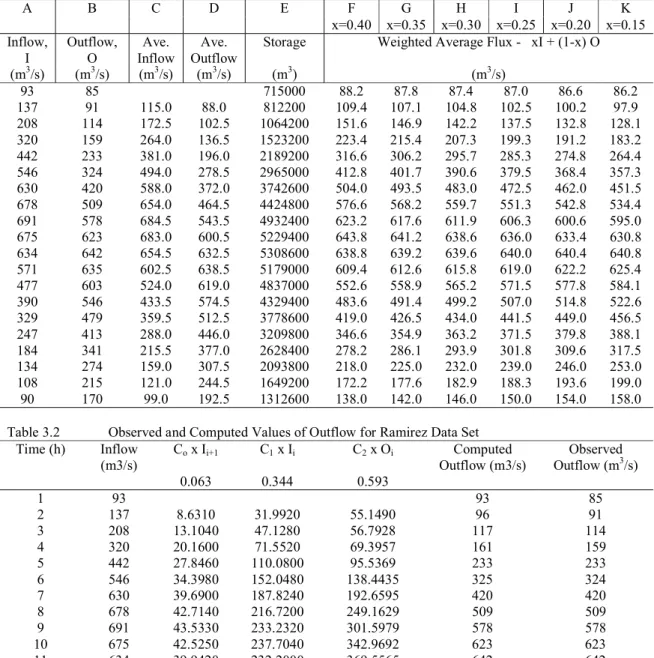
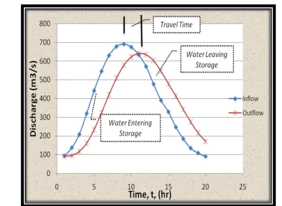
Based on output from spreadsheet (Table 3.1), a value of x = 0.15 gave the straightest loop (Figure 3.1). The best fit to the corresponding points yields a value of k = 2.31 h. Co, C1, and C2 was obtained using equation (2.5), (2.6) and (2.7) respectively (Table 3.2). Figure 3.2 is the hydrograph for the flood routing. For data set 1, table 3.3 gives the estimated value for x while figure 3.3 shows x= 0.555 is the straightest. Table 3.4 is routed data of

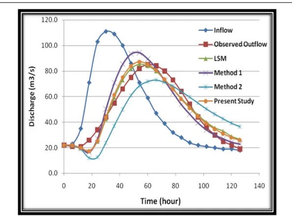
computed outflow and Figure 3.4 compares outflow hydrographs of methods in data set 1.

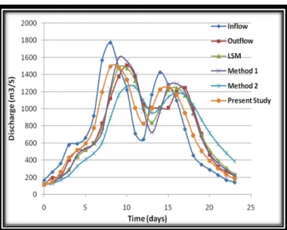
Results for data set 2 is tabulated with observed outflow in Al-Humoud and Esen (Table 3.5 and 3.6). Figure 3.5 gives the narrowest loop at x = 0.25 and final outflow hydrograph is represented in Figure 3.6.

Data Set 3observed and computed values of outflow was routed using values of C0, C1 and C2 (Table 3.8) from value of x = 0.08 (Table 3.7 and Figure 3.7). Figure 3.7 is the plot of storage versus [xI + (1-x) O]. The hydrograph for the flow data is presented in Figure 3.8.

3.2 Statistical Analysis

The routing data for data set 1, 2 and 3 were put side by side with the other estimated values from other authors of the data sets analyzed. Statistical analysis Analysis of Variance (ANOVA) was carried out to compare the means of the four different approaches. The Least Square Method, Method 1, Method 2 and the Present Study were put into statistical perspective. The basic purpose of the analysis of variance is to test the homogeneity of several data; ANOVA is a technique that enables evaluation of several populations means simultaneously (Gupta, 2008).

Null hypotheses: There is no significant difference in the methods

Ho: µ1 = µ2 = µ3 = µ4

Alternative hypotheses: There is a significant difference in the methods

H1: µ1 ≠ µ2 ≠ µ3 ≠ µ4 µ1 = LSM µ2 = Method 1 µ3 = Method 2 µ4 = Present Study Alpha value: 0.01

For data set 1, Variance ratio (F) < Critical value at alpha =0.01. Since the calculated value of the F = 0.104 is less than critical value 4.024 (Table 3.10 and 3.11), it is not significant, hence the Null hypotheses is not rejected at 1 percent level of significance. Therefore there is no significant difference between the LSM, Method 1, Method 2 and the values routed with Muskingum using Microsoft excel in the Present study and conclude with 99 percent confidence level that the methods does not differ significantly. There was also no significant difference with Vatankhah’s (2014) study of “Solving nonlinear Muskingum model by Fourth-Order Runge-Kutta Method” and Chu (2009) using Fuzzy Inference System.

For data set 2, Variance ratio < Critical value at alpha =0.01. Also, the calculated value of the F= 0.015 is less than critical value 4.002, the Null hypotheses is accepted at 1 percent level of significance. Therefore there was no significant difference between the LSM, Method 1, Method 2 and the values routed with Muskingum using Microsoft Excel in the Present study (Table 3.12 and 3.13) and conclude that with 99 percent confidence that the methods has no significant difference.

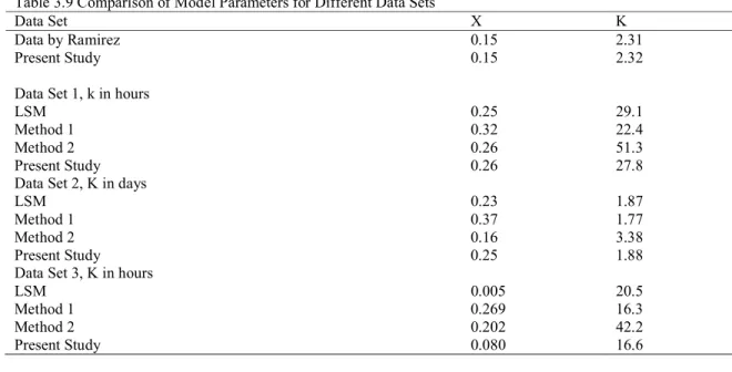
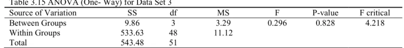
Data set 3 at alpha =0.01, Variance ratio 0.296 is less than critical value 4.018 (Table 3.14 and 3.15), with 99 percent confidence level, it is not significant. For this reason, the Null hypothesis is accepted at 1 percent level of significance and the alternative hypothesis rejected. No significant difference exists between the LSM, Method 1, Method 2 and the outflow values in the Present study. It is therefore concluded with 99 percent certainty that the methods does not differ. Moreover, data set 1, 2, and 3 shows that the model parameter (Table 3.9) results are in good agreement with the observation values and gave more flexible results.

3.3 Limitations to Muskingum Method

Despite the flexibility, simplicity and advantage of this flood routing technique, better knowledge of its limitations can help scientists and hydrologists improved on the generality of models. Some of the shortcomings include:

i. Muskingum method assumes a single stage-discharge relationship. This assumption may not be possible in natural open channel. For instance, the friction slope drawn on the rising limb of the flood hydrograph for a given flow, may be rather dissimilar than for the falling limb of the hydrograph for the same given flow.

Some flood wave may have all the three propagation in the same flow.

 Entire reach flooded I =Q

 Advancing Flood Wave I > Q

 Receding Flood Wave Q > I

ii. Moreover, the method has the drawback of producing a negative initial outflow which is commonly referred to as ‘reduced flow’ at the beginning of the routed hydrograph. This view has been supported in the work of Perumal as cited by Elbashir (2008) and Luo and Xuewei (1987).

iii. This limitation above makes Muskingum not suitable for very steep channel. Thus, it is not applicable to steeply rising hydrographs such as dam breaks.

iv. In many flow cases, K is generally assumes constant for easy computation which may be incorrect at all point of the stream.

v. The method also pays little and sometimes no attention to variable backwater effects such as downstream dam, bridges barrier, wave, human and geological influences.

4.0 CONCLUSION AND RECOMMENDATION

Flood routing using Microsoft excel (spreadsheet) was implemented in this work using Muskingum method for three different popular data sets. In spite of the simplicity of linear method, nonlinear also yielded outflow with no significant difference. Though the method has limitations, it produces similar routing effects according to the values of the available data. It is recommended that future work should dwell on comparing output of other hydraulic and hydrological routing methods in channel routing to Muskingum models so as to improve on routing techniques. More studies on estimating flow routing parameters simultaneously by using Excel Solver should also be conducted.

ACKNOWLEDGEMENT

The authors acknowledge all staff of Department of Civil Engineering, Obafemi Awolowo University, Ile-Ife for their support.

Table 3.1 Values for X computed for Ramirez Data Set

A B C D E F G H I J K x=0.40 x=0.35 x=0.30 x=0.25 x=0.20 x=0.15 Inflow, I Outflow, O Ave. Inflow Ave. Outflow

Storage Weighted Average Flux - xI + (1-x) O

(m3_{/s) (m}3_{/s) (m}3_{/s) (m}3_{/s) (m}3_{) (m}3_/s) 93 85 715000 88.2 87.8 87.4 87.0 86.6 86.2 137 91 115.0 88.0 812200 109.4 107.1 104.8 102.5 100.2 97.9 208 114 172.5 102.5 1064200 151.6 146.9 142.2 137.5 132.8 128.1 320 159 264.0 136.5 1523200 223.4 215.4 207.3 199.3 191.2 183.2 442 233 381.0 196.0 2189200 316.6 306.2 295.7 285.3 274.8 264.4 546 324 494.0 278.5 2965000 412.8 401.7 390.6 379.5 368.4 357.3 630 420 588.0 372.0 3742600 504.0 493.5 483.0 472.5 462.0 451.5 678 509 654.0 464.5 4424800 576.6 568.2 559.7 551.3 542.8 534.4 691 578 684.5 543.5 4932400 623.2 617.6 611.9 606.3 600.6 595.0 675 623 683.0 600.5 5229400 643.8 641.2 638.6 636.0 633.4 630.8 634 642 654.5 632.5 5308600 638.8 639.2 639.6 640.0 640.4 640.8 571 635 602.5 638.5 5179000 609.4 612.6 615.8 619.0 622.2 625.4 477 603 524.0 619.0 4837000 552.6 558.9 565.2 571.5 577.8 584.1 390 546 433.5 574.5 4329400 483.6 491.4 499.2 507.0 514.8 522.6 329 479 359.5 512.5 3778600 419.0 426.5 434.0 441.5 449.0 456.5 247 413 288.0 446.0 3209800 346.6 354.9 363.2 371.5 379.8 388.1 184 341 215.5 377.0 2628400 278.2 286.1 293.9 301.8 309.6 317.5 134 274 159.0 307.5 2093800 218.0 225.0 232.0 239.0 246.0 253.0 108 215 121.0 244.5 1649200 172.2 177.6 182.9 188.3 193.6 199.0 90 170 99.0 192.5 1312600 138.0 142.0 146.0 150.0 154.0 158.0

Table 3.2 Observed and Computed Values of Outflow for Ramirez Data Set Time (h) Inflow

(m3/s) Co x Ii+1 C1 x Ii C2 x Oi Outflow (m3/s) Computed Outflow (mObserved 3_/s)

0.063 0.344 0.593 1 93 93 85 2 137 8.6310 31.9920 55.1490 96 91 3 208 13.1040 47.1280 56.7928 117 114 4 320 20.1600 71.5520 69.3957 161 159 5 442 27.8460 110.0800 95.5369 233 233 6 546 34.3980 152.0480 138.4435 325 324 7 630 39.6900 187.8240 192.6595 420 420 8 678 42.7140 216.7200 249.1629 509 509 9 691 43.5330 233.2320 301.5979 578 578 10 675 42.5250 237.7040 342.9692 623 623 11 634 39.9420 232.2000 369.5565 642 642

12 571 35.9730 218.0960 380.5272 635 635 13 477 30.0510 196.4240 376.3156 603 603 14 390 24.5700 164.0880 357.4548 546 546 15 329 20.7270 134.1600 323.8449 479 479 16 247 15.5610 113.1760 283.8880 413 413 17 184 11.5920 84.9680 244.6866 341 341 18 134 8.4420 63.2960 202.3593 274 274 19 108 6.8040 46.0960 162.5397 215 215 20 90 5.6700 37.1520 127.7557 171 170

Figure 3.2 Storage versus the storage discharge Data Set 1

Table 1.4 Estimated value of x for Data set 1

A B C D E F G H I J K

x=0.40 x=0.35 x=0.30 x=0.20 x=0.26 x=0.25 Inflow, Outflow Ave.

Inflow

Ave. Outflow

Storage Weighted Average Flux - xI + (1-x) O

(m3_{/s) (m}3_{/s) (m}3_{/s) (m}3_{/s) (m}3_{) (m}3_/s) 22 22 21600 22.0 22.0 22.0 22.0 22.0 22.0 23 21 22.5 21.5 43200 21.8 21.7 21.6 21.4 21.5 21.5 35 21 29.0 21.0 216000 26.6 25.9 25.2 23.8 24.6 24.5 71 26 53.0 23.5 853200 44.0 41.8 39.5 35.0 37.7 37.3 103 34 87.0 30.0 2084400 61.6 58.2 54.7 47.8 51.9 51.3 111 44 107.0 39.0 3553200 70.8 67.5 64.1 57.4 61.4 60.8 109 55 110.0 49.5 4860000 76.6 73.9 71.2 65.8 69.0 68.5 100 66 104.5 60.5 5810400 79.6 77.9 76.2 72.8 74.8 74.5 86 75 93.0 70.5 6296400 79.4 78.9 78.3 77.2 77.9 77.8 71 82 78.5 78.5 6296400 77.6 78.2 78.7 79.8 79.1 79.3 59 85 65.0 83.5 5896800 74.6 75.9 77.2 79.8 78.2 78.5 47 84 53.0 84.5 5216400 69.2 71.1 72.9 76.6 74.4 74.8 39 80 43.0 82.0 4374000 63.6 65.7 67.7 71.8 69.3 69.8 32 73 35.5 76.5 3488400 56.6 58.7 60.7 64.8 62.3 62.8 28 64 30.0 68.5 2656800 49.6 51.4 53.2 56.8 54.6 55.0 24 54 26.0 59.0 1944000 42.0 43.5 45.0 48.0 46.2 46.5 22 44 23.0 49.0 1382400 35.2 36.3 37.4 39.6 38.3 38.5 21 36 21.5 40.0 982800 30.0 30.8 31.5 33.0 32.1 32.3 20 30 20.5 33.0 712800 26.0 26.5 27.0 28.0 27.4 27.5 19 25 19.5 27.5 540000 22.6 22.9 23.2 23.8 23.4 23.5 19 22 19.0 23.5 442800 20.8 21.0 21.1 21.4 21.2 21.3 18 19 18.5 20.5 399600 18.6 18.7 18.7 18.8 18.7 18.8

Table 3.4 Observed and Computed Values of Outflow for Data Set 1 Time

(h) Inflow (m3/s) Observed Outflow (m3/s) Computed O (m3/s) Co x Ii+1 C1 x Ii C2x Oi (m3/s) (m3/s) (m3/s) LSM Method 1 Method 2 Present Study (-) 0.179 0.434 0.745 0 22.0 22.0 22.0 22.0 22.0 22.0 6 23.0 21.0 21.8 21.8 21.7 21.8 4.117 9.548 16.390 12 35.0 21.0 20.0 19.5 18.9 20.0 6.265 9.982 16.257 18 71.0 26.0 17.5 16.4 12.0 17.4 12.709 15.190 14.880 24 103.0 34.0 24.9 27.1 12.5 25.3 18.437 30.814 12.934 30 111.0 44.0 42.4 50.2 23.8 43.7 19.869 44.702 18.857 36 109.0 55.0 59.3 70.6 37.1 61.2 19.511 48.174 32.549 42 100.0 66.0 72.9 85.3 49.9 75.0 17.900 47.306 45.603 48 86.0 75.0 81.8 93.3 60.9 83.9 15.394 43.400 55.882 54 71.0 82.0 85.4 94.3 68.4 87.1 12.709 37.324 62.496 60 59.0 85.0 84.0 89.3 71.8 85.2 10.561 30.814 64.898 66 47.0 84.0 80.0 82.1 73.0 80.6 8.413 25.606 63.437 72 39.0 80.0 73.4 72.4 71.2 73.5 6.981 20.398 60.070 78 32.0 73.0 66.3 63.0 68.3 65.9 5.728 16.926 54.748 84 28.0 64.0 58.7 53.7 64.0 58.0 5.012 13.888 49.129 90 24.0 54.0 52.0 46.2 59.7 51.1 4.296 12.152 43.214 96 22.0 44.0 45.6 39.3 55.0 44.5 3.938 10.416 38.047 102 21.0 36.0 40.0 33.9 50.4 39.0 3.759 9.548 33.171 108 20.0 30.0 35.6 29.9 46.3 34.6 3.580 9.114 29.025 114 19.0 25.0 33.0 26.9 42.7 31.0 3.401 8.680 25.747 120 19.0 22.0 28.9 24.3 39.2 28.0 3.401 8.246 23.114 126 18.0 19.0 26.6 22.8 36.5 25.9 3.222 8.246 20.830

Figure 3.4 Outflow hydrographs for the data set 1 four methods Data Set 2

Table 3.5 Estimated value of x for Data Set 2

A B C D E F G H I x=0.40 x=0.35 x=0.30 x=0.25 Inflow, I

(m3_/s) Outflow, _{O (m}3_{/s) Inflow} Ave.

(m3_/s)

Ave. Outflow

(m3_/s)

Storage (m3_{) Weighted Average Flux -}

xI + (1-x) O 166.2 118.4 4924800 137.5 135.1 132.7 130.4 263.6 197.4 214.9 157.9 9849600 223.9 220.6 217.3 214.0 365.3 214.1 314.5 205.8 19241280 274.6 267.0 259.5 251.9 580.5 402.1 472.9 308.1 33480000 473.5 464.5 455.6 446.7 594.7 518.2 587.6 460.2 44491680 548.8 545.0 541.2 537.3 662.6 523.9 628.7 521.1 53788320 579.4 572.4 565.5 558.6 920.3 603.1 791.5 563.5 73483200 730.0 714.1 698.3 682.4 1568.8 829.7 1244.6 716.4 119115360 1125.3 1088.4 1051.4 1014.5 1775.5 1124.2 1672.2 977.0 179180640 1384.7 1352.2 1319.6 1287.0 1489.5 1379.0 1632.5 1251.6 212090400 1423.2 1417.7 1412.2 1406.6 1223.3 1509.3 1356.4 1444.2 204508800 1394.9 1409.2 1423.5 1437.8 713.6 1379.0 968.5 1444.2 163408320 1112.8 1146.1 1179.4 1212.7 645.6 1050.6 679.6 1214.8 117167040 888.6 908.9 929.1 949.4 1166.7 1013.7 906.2 1032.2 106280640 1074.9 1067.3 1059.6 1052.0 1427.2 1013.7 1297.0 1013.7 130753440 1179.1 1158.4 1137.8 1117.1 1282.8 1013.7 1355.0 1013.7 160241760 1121.3 1107.9 1094.4 1081.0 1098.7 1209.1 1190.8 1111.4 167097600 1164.9 1170.5 1176.0 1181.5 764.6 1248.8 931.7 1229.0 141410880 1055.1 1079.3 1103.5 1127.8 458.7 1002.4 611.7 1125.6 97005600 784.9 812.1 839.3 866.5 351.1 713.6 404.9 858.0 57857760 568.6 586.7 604.9 623.0 288.8 464.4 320.0 589.0 34611840 394.2 402.9 411.7 420.5 228.8 325.6 258.8 395.0 22844160 286.9 291.7 296.6 301.4 170.2 265.6 199.5 295.6 14541120 227.4 232.2 237.0 241.8 143.0 222.6 156.6 244.1 6981120 190.8 194.7 198.7 202.7

Time (days) Inflow (m3/s) Outflow (m3/s) Outflow (m3/s) Co x Ii+1 (m3_{/s) (m}C1 x I3_/s) i C_(m2 x O3_/s) i LSM Method

1 Method 2 Present Study

0.016 0.508 0.476 0 166.2 118.4 118.4 118.4 118.4 118.4 1 263.6 197.4 146.1 138.7 131.6 146.6 5.845 84.430 56.358 2 365.3 214.1 209.6 206.3 170.0 264.7 9.288 185.572 69.797 3 580.5 402.1 296.4 284.1 226.0 430.4 9.515 294.894 125.977 4 594.7 518.2 442.2 466.3 331.9 517.6 10.602 302.108 204.864 5 662.6 523.9 522.4 539.3 409.8 597.7 14.725 336.601 246.365 6 920.3 603.1 602.7 590.9 482.5 777.1 25.101 467.512 284.501 7 1569 829.7 786.8 732.7 606.2 1195.3 28.408 796.950 369.906 8 1776 1124.2 1193.6 1230.5 891.9 1494.7 23.832 901.954 568.946 9 1490 1379.0 1481.7 1595.4 1159.4 1487.7 19.573 756.666 711.492 10 1223 1509.3 1476.8 1555.4 1261.2 1341.0 11.418 621.436 708.160 11 713.6 1379.0 1330.1 1398.6 1255.5 1011.2 10.330 362.509 638.323 12 645.6 1050.6 1012.5 981.0 1094.2 827.9 18.667 327.965 481.313 13 1167 1013.7 842.3 723.4 954.1 1009.6 22.835 592.684 394.102 14 1427 1013.7 1016.9 972.9 1014.8 1226.1 20.525 725.018 480.579 15 1283 1013.7 1221.9 1268.0 1139.8 1252.9 17.579 651.662 583.634 16 1099 1209.1 1246.9 1294.8 1184.6 1166.7 12.234 558.140 596.369 17 764.6 1248.8 1160.0 1205.4 1162.7 951.1 7.339 388.417 555.369 18 458.7 1002.4 947.5 961.8 1047.0 691.4 5.618 233.020 452.736 19 351.1 713.6 693.9 660.6 872.2 512.1 4.621 178.359 329.093 20 288.8 464.4 516.5 475.0 717.0 394.1 3.661 146.710 243.747 21 228.8 325.6 398.1 365.5 589.6 306.6 2.723 116.230 187.600 22 170.2 265.6 309.5 286.5 482.3 234.7 2.288 86.462 145.920 23 143.0 222.6 237.4 217.1 389.2 184.3 0.000 72.644 111.703

Figure 3.6 Outflow hydrographs for the data set 2 methods Data Set 3

Table 3.7 Estimated value of x for Data Set 3

A B C D E F G H I J

x=0.20 x=0.15 x=0.10 x=0.05 x=0.08 Inflow, I Outflow,

O Inflow Ave. Outflow Ave. Storage Weighted Average Flux - xI + (1-x) O

(m3_{/s) (m}3_{/s) (m}3_{/s) (m}3_{/s) (m}3_{) (m}3_/s) 1.87 1.87 45360 1.9 1.9 1.9 1.9 1.9 7.08 2.89 4.5 2.4 90612 3.7 3.5 3.3 3.1 3.2 15.57 5.24 11.3 4.1 247428 7.3 6.8 6.3 5.8 6.1 18.85 7.50 17.2 6.4 481572 9.8 9.2 8.6 8.1 8.4 11.89 9.49 15.4 8.5 630072 10.0 9.9 9.7 9.6 9.7 8.35 10.48 10.1 10.0 632988 10.1 10.2 10.3 10.4 10.3 5.95 10.42 7.2 10.5 561708 9.5 9.7 10.0 10.2 10.1 4.16 8.78 5.1 9.6 463536 7.9 8.1 8.3 8.5 8.4 2.83 6.94 3.5 7.9 369252 6.1 6.3 6.5 6.7 6.6 2.10 5.66 2.5 6.3 286416 4.9 5.1 5.3 5.5 5.4 1.70 4.67 1.9 5.2 215892 4.1 4.2 4.4 4.5 4.4 1.44 3.74 1.6 4.2 158976 3.3 3.4 3.5 3.6 3.6 1.30 2.83 1.4 3.3 117612 2.5 2.6 2.7 2.8 2.7

Table 3.8 Observed and Computed Values of Outflow for Data Set 3 Time

(hours) Inflow (m3/s) Observed Outflow (m3/s)

Computed Outflow (m3/s) Co x Ii+1 C1 x Ii C2 x Oi

LSM Method 1 Method 2 Present

Study 0.092 0.237 0.672 0 1.87 1.87 1.87 1.87 1.87 1.87 6 7.08 2.89 2.31 1.39 1.09 2.35 0.651 0.443 1.257 12 15.57 5.24 4.32 2.89 0.79 4.69 1.432 1.678 1.580 18 18.85 7.50 7.61 7.69 2.71 8.58 1.734 3.690 3.152 24 11.89 9.49 10.02 12.82 6.40 11.32 1.094 4.467 5.763 30 8.35 10.48 10.22 12.78 7.83 11.20 0.768 2.818 7.610 36 5.95 10.42 9.52 11.22 8.28 10.05 0.547 1.979 7.524 42 4.16 8.78 8.41 9.27 8.17 8.55 0.383 1.410 6.754 48 2.83 6.94 7.16 7.34 7.71 6.99 0.260 0.986 5.743 54 2.10 5.66 5.94 5.59 7.02 5.56 0.193 0.671 4.697 60 1.70 4.67 4.88 4.22 6.28 4.39 0.156 0.498 3.737 66 1.44 3.74 4.00 3.23 5.57 3.49 0.132 0.403 2.951 72 1.30 2.83 3.31 2.52 4.91 2.80 0.120 0.341 2.343

Figure 3.7 Graph of Storage versus [xI + (1-x) O] at different value of x

Table 3.9 Comparison of Model Parameters for Different Data Sets

Data Set X K

Data by Ramirez 0.15 2.31

Present Study 0.15 2.32

Data Set 1, k in hours

LSM 0.25 29.1

Method 1 0.32 22.4

Method 2 0.26 51.3

Present Study 0.26 27.8

Data Set 2, K in days

LSM 0.23 1.87

Method 1 0.37 1.77

Method 2 0.16 3.38

Present Study 0.25 1.88

Data Set 3, K in hours

LSM 0.005 20.5

Method 1 0.269 16.3

Method 2 0.202 42.2

Present Study 0.080 16.6

Table 3.10 Summary of Data Set 1

Groups Count Sum Average Variance

LSM 22 1072.10 48.73 553.36

Method 1 22 1084.30 49.29 745.00

Method 2 22 1005.30 45.70 417.84

Present Study 22 1074.55 48.84 585.98

Table 3.11 ANOVA (One- Way) for Data Set 1

Source of Variation SS df MS F value P- Critical F

Between Groups 178.96 3 59.65 0.104 0.958 4.024

Within Groups 48345.86 84 575.55

Total 48524.82 87

Table 3.12 Summary of Data Set 2

Groups Count Sum Average Variance

LSM 24 18210.20 758.76 195206.12

Method 1 24 18268.60 761.19 221700.09

Method 2 24 17691.90 737.16 154301.17

Present Study 24 18139.92 755.83 201239.51

Table 3.13 Anova (One- Way) for Data Set 2

Source of Variation SS Df MS F P-value F critical

Between Groups 8613.00 3 2871 0.015 0.998 4.002

Within Groups 17766278.47 92 193112

Table 3.14 Summary of Data Set 3

Groups Count Sum Average Variance

LSM 13 79.57 6.12 8.49

Method 1 13 82.83 6.37 17.03

Method 2 13 68.63 5.28 7.60

Present Study 13 81.84 6.30 11.34

Table 3.15 ANOVA (One- Way) for Data Set 3

Source of Variation SS df MS F P-value F critical

Between Groups 9.86 3 3.29 0.296 0.828 4.218

Within Groups 533.63 48 11.12

Total 543.48 51

REFRENCES

Al-Humond J., M., and Esen, I. (2006). Approximate method for the estimation of Muskingum flood routing parameters. Springer, 20:979-990. DOI: 10.1007/s11269-006-9018-2

Barati, R. (2011). “Parameter estimation of nonlinear Muskingum models using Nelder-Mead simplex algorithm.” Journal of Hydrologic Engineering, ASCE, Vol. 16, No. 11, pp. 946-954.

Barati, R. (2013). Application of Excel Solver for Parameter Estimation of the Nonlinear Muskingum Models.

KSCE Journal of Civil Engineering, 17 (5), 1139-1148. DOI 10.1007/s12205-013-0037-2 Boyd, C., Yoo, K. (1994) Hydrology and water supply for pond aquaculture, New York: Champan & Hall. Chin, D. (2000) Water Resources Engineering, New Jersey: Prentice Hall.

Chow V. T., (ed.) (1964). Handbook of Applied Hydrology. New York: McGraw Hill.

Chu, H.-J. (2009). The Muskingum Flood Routing Model using a Neuro Fuzzy Approach. KSCE Journal of Civil Engineering , 13 (5), 371-376. DOI 10.1007/s12205-009-0371-6

Elbashir, S. T. (2011). Flood Routing in Natural Channels Using Muskingum Methods. Dublin Institute of Technology, Civil and Environmental Engineering Commons. Dublin: School of Civil and Building Services Engineering .

Guo, J. (2006) Urban Hydrology and Hydraulic Design, Highlands Ranch: Water Resources Publications, LLC. Gupta, S. C., (2008). Fundamentals of Statistics (Sixth ed.). (I. Gupta, Ed.) New Delhi, India: Himalaya

Publishing House.

Haan, C., Barfield, B., Hayes, J. (1994) Design hydrology and sedimentology for small Catchments, San Diego: ACADEMIC PRESS. INC.

Hamedi, F., Haddad, B. O., and Orouji, H. (2014). Discussion of “Application of Excel Solver for Parameter Estimation of. KSCE Journal of Civil Engineering . DOI 10.1007/s12205-014-0566-3

Karahan, H. (2009). Predicting Muskingum Flood Routing Parameters Using Spreadsheet. Pamukkale University, Department of Civil Engineering,. Denizli, Turkey: Pamukkale University.

Kim, J. H., Geem, W. G. and Kim, E. S. (2001). Parameter Estimation of the Nonlinear Muskingum Model Using Harmony Search. Journal of the American Water Resources Association, 37 (5).

Luo, B., and Xuewei, Q. (1987). Some Problems with the Muskingum Method. Hydrological Sciences - Journal- des Sciences Hydrologiques .

Mays, L.W., and Tung, Y. (2002) Hydro-systems engineering and management, Highlands Ranch: Water Resources Publications, LLC.

Ramírez, J. A. (2000) Prediction and Modeling of Flood Hydrology and Hydraulics. Chapter 11 of Inland Flood Hazards: Human, Riparian and Aquatic Communities Eds. Ellen Wohl; Cambridge University Press. Tung, Y. K. (1985). River Flood Routing by Nonlinear Muskingum Method. ASCE Journal of Hydraulic

Engineering 111(12):1447-1460.

Vatankhah, A. R. (2014, July 7). Discussion of “Application of Excel Solver for Parameter Estimation of the Nonlinear Muskingum Models” by Reza Barati. KSCE Journal of Civil Engineering. DOI 10.1007/s12205-014-1422-1