Minimum pricing of alcohol and its impact on consumption in the UK
Matthieu Arnoult
†& Richard Tiffin
‡† Land Economy and Environment Research Group, Scottish Agricultural College King’s Buildings, EH9 3JG Edinburgh – [email protected] ‡ Department of Agricultural & Food Economics, The University of Reading
Whiteknights, PO Box 237, RG6 6AR Reading – [email protected]
Abstract
A complete model of food demand is estimated for UK households, focusing on alcohol consumption both at home and outside.
Using EFS data for 2005-06, several AIDS models have been estimated at different aggregation levels, thus defining a hierarchical system which allows for computation of cross elasticities between finely disaggregated food groups. At the bottom level of the system, elasticities for 9 groups of alcoholic drinks are computed, 4 of which corresponding to home consumption, 5 corresponding to outside consumption. Estimates from the upper levels of aggregation are used to acknowledge substitution and complementarity effect between these 9 groups and all other food groups consumed.
Based on alcohol content of the different drinks studied, their strength and price per unit of alcohol sold is computed; a price increase is then devised, whereby all drinks must be sold at a minimum price of 50p per unit. This rise in alcohol prices, in combination with price elasticities of demand, indicates consumption changes observed according to different socio-economic characteristics (geographical, age, gender, income, socio-economic group).
In spite of a slight substitution effect between alcoholic drinks and other food groups, overall consumption would decrease by 15% at the UK level. Only alcohol sold for home consumption would see an increase in prices, and reduction in sales would generally spare pubs and restaurants. While consuming more units of alcohol than other groups, higher income and high managerial groups would be less affected by this pricing policy.
Paper presented at the 84th Annual Conference of the Agricultural Economics Society 29—31 March 2010, Pollocks Hall, Edinburgh
1.
Introduction
The direct impact of alcohol abuse at the individual level is well documented, with short-term effects ranging from intoxication and dehydration to sleep disruption and fatigue (NHS, 2010). Sustained consumption over a long period lead to more severe and possibly lethal consequences, with increased risks of cancers (e.g., mouth, liver) or heart conditions (e.g., stroke, high blood pressure) among other possible outcomes (NHS, 2010). Indirect influence of alcohol consumption is also debated, with the Chief Medical Officer (CMO) for England likening it to second-hand smoking (DH, 2008), whereby alcohol abusers are endangering not only themselves but also their entourage through, for example, harm to an unborn foetus, violence and vandalism and society as a whole through the health burden carried by public health services and other indirect costs to the economy. There has been a secular increase in alcohol consumption in the UK over recent decades: annual UK consumption per person aged 15 and over was estimated at 11.37 litres per person over 15 in 2003, 34% more than it was in 1970 (WHO, 2010). In comparison, consumption in other European countries such as France or Germany, whilst still slightly higher than in the UK (respectively 12.25 and 12.66 litres), has been decreasing over the same period (-47% and -18% respectively). At the EU-15 level, average consumption is 11.43 litres per person, a 27% decrease since 1970. At the same time the affordability of alcohol has increased. Over the period 1980-2006, the average price of alcohol by 65%, while households’ real disposable income almost doubled (ONS-NHS, 2007). These changes have been accompanied by a twofold increase in alcohol-related deaths in the United Kingdom between 1991 and 2008 (ONS, 2010). In the case of a specific alcohol-related condition such as cirrhosis, Leon and McCambridge (2006a & 2006b) report a five-fold increase in the mortality rate for men aged 15-44 in England and Wales between 1950 and 2002 with an on-going upward trend, while other in other European countries their incidence is declining.
Statistics such as these have prompted government actions over the last few years. The Licensing Act 2003 which came into force in late 2005 in England and Wales, introduced an extension of licensing hours, in order to foster a more continental approach to drinking (DCMS, 2008). For over two decades, the Department of Health and NHS have been advocating responsible consumption through ad campaigns such as “Know your limits” and “Drinkaware” and the promotion of guidelines based on unit equivalents of alcoholic drinks. The latest policy instrument being debated, particularly in Scotland, is a price floor on alcohol as suggested by the Chief Medical Officer for England (DH, 2008). This policy is based on the so-called Sheffield Study (Booth et al., 2008) which used a meta-analysis to estimate the health impact of an increase in alcohol prices; results indicate
that such a policy would affect heavy drinkers more than others, and could potentially save 3,400 lives annually in England within 10 years of its implementation (DH, 2008).
A minimum price of 50p per unit has been suggested. The Department of Health defines 1 unit of alcohol as 10ml equivalent to 8g of pure ethanol, which is equivalent to 1 litre of an alcoholic drink at 1% alcohol by volume (ABV). Thus, the proposed minimum price would lead to prices of £1.10 and 92p for a 440ml can of Stella Artois and Guinness respectively, £5.25 for a bottle of Californian Merlot and £14.00 for a bottle of Whisky.
We conduct an analysis of the impacts of a change in alcohol prices. Unlike Booth et al. we use a model which does exclusively focus on the demand for alcoholic beverages. The model is estimated using household data from the UK Expenditure and Food Survey (EFS). Household data as provided are too imprecise to assess individuals’ consumption and its subsequent health effects; our primary aim is therefore to estimate possible shifts in expenditure on alcoholic drinks triggered by any price increase, and the redistribution effects this would entail across all food expenditures, a fact which cannot be assessed from meta-studies focusing only on alcohol. We further investigate the distributional effects across various socio-demographic characteristics of the sample, by estimating expenditure elasticities for each category, with particular attention to less affluent households.
2.
Methods
We estimate a full demand system using the Expenditure and Food Survey for 2005-2006. Over a two-week period, 6750 households recorded a detailed diary of their food and drinks purchases in terms of both quantities and expenditures. The number of food items in those diaries is in excess of 500, thus providing a very detailed breakdown of food intake at the household level. In the case of alcoholic drinks, the data distinguishes 25 different products, consumed either at home or outside of home (that is, purchased from and consumed within leisure venues such as pubs and restaurants). Our model employs the widely used Almost Ideal Demand System (Deaton and Muellbauer, 1980a & 1980b) which is represented as follows:
(1)
(2)
(3)
where is the share of total expenditure accounted for by expenditure on the good in the household, is the price of the good to the household, is Stone’s price index and is a vector of variables that describes the household’s socio-demographic characteristics. An important consideration when estimating demand models is the treatment of censored observations where the level of consumption of a particular good in a household is zero during the survey period. In order to address this we employ a version of the Infrequency of Purchase Model (IPM) introduced by Blundell and Meghir (1987).1
It is not possible to estimate a single model comprising of all the food items required in our analysis. It is however possible to estimate models comprising of only a few groups of foods and drinks at a time, for instance, table wine, sparkling wine and fortified wine can be modelled using a “wine” model. In so doing however it is assumed that expenditure on a given category of food remains constant. For example, when looking at the effects of a change in the price of red wine on consumption, it would be assumed that the price change does not induce a change in expenditure on the category as a whole. Since this is unrealistic we resort to a hierarchical approach in which introduces an additional layer to the model in which the effects of a change in a component price within a category (e.g., wine) on overall expenditure on the category are measured.
1
All food items are included in a hierarchical system whereby food groups are disaggregated into smaller groups from the top down. The top level of the system includes all commodities, aggregated into 5 major groups: dairy, fats & eggs, meat & fish, cereal products & potatoes, fruit & vegetables, and drinks. The intermediate level breaks down the drinks group further into 4 subgroups: tea & coffee, soft drinks, alcohol ‘in’ and alcohol ‘out’. The latter two groups refer to alcoholic drinks consumed at home and those consumed away from home. At the bottom level alcohol ‘in’ is split into beer & lager, alcopops, cider & mixers, wines, and spirits & liqueurs, while the alcohol ‘out’ group comprises of bitter, cider & alcopops, lager & other beers, wines, and spirits & liqueurs. Four models are estimated, providing 4 independent sets of own- and cross-price elasticities. Following Edgerton (1997), the full matrix of elasticities for alcoholic drinks is computed, taking into account the effects of changing prices on group specific expenditure, as well as substitution and complementarity effects betweens food groups.
Using drink-specific alcohol content provided by the EFS, the units of alcohol purchased by a household can be derived from observed quantities of the drinks purchased, assuming that 1 unit is equivalent to 8g of pure alcohol. The price per unit of alcohol is then computed based on the expenditure recorded in the survey. Where this falls short of the 50p threshold, the price is increased to the threshold, and the overall impact on alcohol consumption is obtained using elasticity estimates. Household-specific socio-demographic information is included at each step of the analysis (elasticity estimation, alcohol consumption patterns, expected price rise), thus providing detailed results along social features of the sample, such as age, gender and ethnic group of the head of household, income tercile, socio-economic group, country or region within the United Kingdom.
3.
Observed Consumption
3.1.
Consumption patterns
Table 1 summarises alcohol consumption recorded in the EFS. On average each household consumes 31.2 units per household per week, with approximately two-thirds consumed at home and one-third consumed away from home. About one third of the intake is due to wine at home (10.4 units), followed by lager out of home (6.3 units), spirits and beer at home (5.0 and 4.9 units respectively), and bitter away from home (2.1 units).
Table 1: General consumption patterns according to alcoholic drinks (units per household per week).
Mean Highest intake Lowest intake
IN
Beer 4.9 7.6 children, 3+ ad 2.4 students
Alcopops 1.0 3.4 unemployed 0.1 asian
Wine 10.4 16.3 high manag. 4.1 unemployed
Spirit 5.0 8.6 Scotland 2.8 black
O
U
T
Bitter 2.1 3.7 Yorks & H 0.4 single parents
Cider 0.5 2.1 children, 3+ ad 0.1 black
Lager 6.3 16.0 3+ adults 2.0 black
Wine 0.8 1.4 high manag. 0.2 black
Spirit 0.2 0.9 students 0.1 black
In home 21.3 26.6 high manag. 13.0 black
Outside 9.9 22.5 3+ adults 3.0 black
Ratio
outside/total 32% 51% 3+ adults 19% black
Overall 31.2 43.8 3+ adults 16.1 black
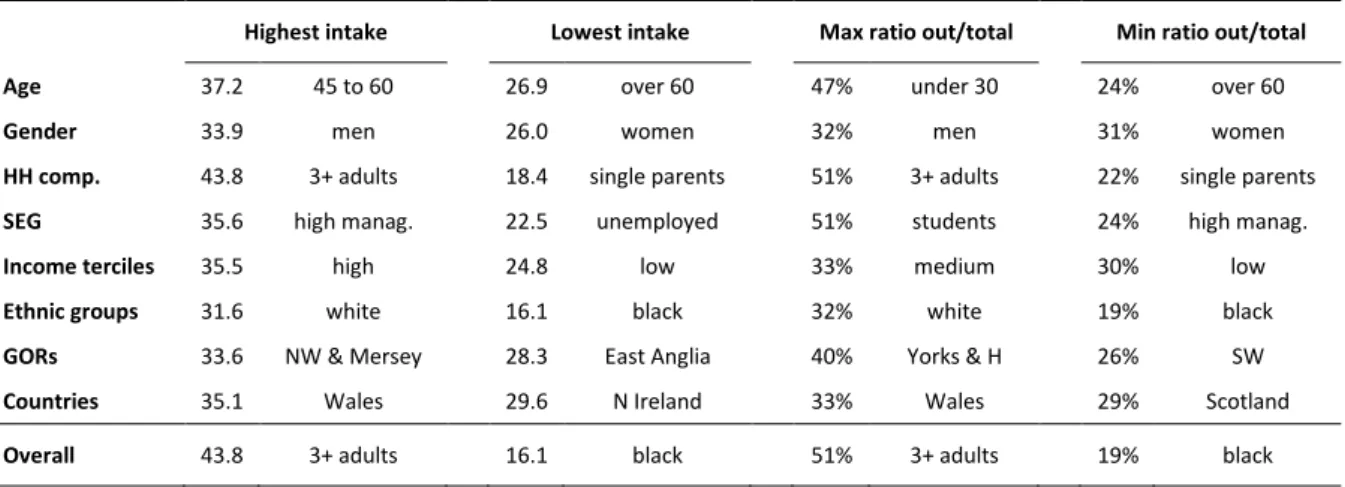
Contrasting intake levels are observed for various socio-demographic groups, as can be seen in Table 2. Regarding the age of the main person responsible for purchases, consumption peaks between 45 and 60, while it is lowest beyond 60. This could however be linked to the presence of aging children, and their later departure from the household. In terms of where consumption takes place, it is maybe unsurprisingly among the under 30 that intake outside of home is highest (47% of total intake), and over 60 that it is lowest (24%).
Household composition results indicate that household comprising of 3 or more adults and no children have the highest intake and highest consumption outside of home (43.8 units and 51%), while single parents have the lowest overall consumption and outside consumption (18.4 units and 22%).
Table 2: Consumption patterns for socio-demographics groups of the sample (units per household and per week).
Highest intake Lowest intake Max ratio out/total Min ratio out/total Age 37.2 45 to 60 26.9 over 60 47% under 30 24% over 60
Gender 33.9 men 26.0 women 32% men 31% women
HH comp. 43.8 3+ adults 18.4 single parents 51% 3+ adults 22% single parents
SEG 35.6 high manag. 22.5 unemployed 51% students 24% high manag.
Income terciles 35.5 high 24.8 low 33% medium 30% low
Ethnic groups 31.6 white 16.1 black 32% white 19% black
GORs 33.6 NW & Mersey 28.3 East Anglia 40% Yorks & H 26% SW
Countries 35.1 Wales 29.6 N Ireland 33% Wales 29% Scotland
Overall 43.8 3+ adults 16.1 black 51% 3+ adults 19% black
Regarding socio-economic groups, high managerial have the highest intake, but the lowest outside of home consumption (35.6 units and 24%), while lowest intake is observed for unemployed (22.5 units) and maximum outside consumption is associated to students (51%). As for income, the high tercile has the highest intake (35.5 units), the medium tercile has the highest outside of home intake (33%), and the low tercile has both lowest intake (24.8 units) and lowest consumption outside of home (30%).
Ethnic groups also exhibit different drinking patterns, with white households having both the highest intake and highest outside of home consumption (31.6 units and 32%), while black have the lowest intake and out of home consumption (16.1 units and 19%).
Regarding regional characteristics in England, northern government office regions have the highest unit intake (North West & Merseyside, 33.6 units) and highest outside of home consumption (Yorkshire & Humber, 40%), while East Anglia has the lowest intake (28.3 units) and the South West the lowest outside of home consumption (26%). As for countries within the UK, Wales has both the highest intake and highest outside of home consumption (35.1 units, 33%), while Northern Ireland has the lowest intake (29.6 units) and Scotland the lowest outside of home consumption (29%).
3.2.
Observed Prices
The mean unit price of alcohol observed in the EFS is 66 pence per unit (ppu), with a mean price of 42ppu for home consumption, and 116ppu outside of home (see Table 3). Regarding alcohol consumed at home, no observed price reaches the threshold of 50ppu, ranging from 33ppu for spirits, up to 47ppu for wine; for alcohol consumed away from home however, the lowest observed price is well above the threshold (89ppu for bitter), while wine reaches a high 248ppu.
Table 3: Unit prices observed in the EFS according to alcoholic drinks (pence per unit of alcohol).
Mean Highest price Lowest price
IN
Beer 43.1 56.8 ethnic other 39.6 E Midlands
Alcopops 35.7 84.7 asian 23.4 ethnic other
Wine 46.5 56.5 ethnic other 36.2 unemployed
Spirit 33.3 40.9 students 27.9 unemployed
O
U
T
Bitter 89.3 103.3 ethnic other 69.4 ethnic mixed
Cider 122.3 150.5 black 78.1 ethnic mixed
Lager 106.1 143.0 ethnic other 92.8 Wales
Wine 248.0 388.3 asian 166.4 ethnic other
Spirit 186.6 372.5 black 146.5 ethnic other
In home 42.1 49.8 London 35.7 unemployed
Outside 116.2 142.9 asian 98.7 NW & Mersey
Ratio
outside/total 56% 76% students 38% black
Overall 65.6 81.7 students 56.4 over 60
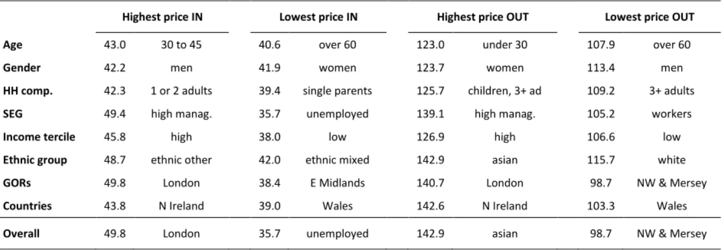
With respect to socio-demographic characteristics of the sample (see Table 4), a few points can be made. The national picture is reproduced regionally with the highest price for a unit of alcohol consumed at home falling short of the limit, at 49.8 pence in London, and the lowest observed price for a unit of alcohol consumed away from home above the threshold at 98.7ppu in the North West & Merseyside. When looking at the share between home and outside, 56% of expenditures on alcohol are on consumption outside of home.
Regarding age, younger people tend to pay higher prices both for alcohol consumed both at and away from of home, while people over 60 always opt for lower prices. In a similar fashion, high managerial classes pay a higher price both in and outside of home, whilst households employed in
Table 4: Unit prices according to socio-demographic features of the sample (pence per unit of alcohol)
Highest price IN Lowest price IN Highest price OUT Lowest price OUT
Age 43.0 30 to 45 40.6 over 60 123.0 under 30 107.9 over 60
Gender 42.2 men 41.9 women 123.7 women 113.4 men
HH comp. 42.3 1 or 2 adults 39.4 single parents 125.7 children, 3+ ad 109.2 3+ adults
SEG 49.4 high manag. 35.7 unemployed 139.1 high manag. 105.2 workers
Income tercile 45.8 high 38.0 low 126.9 high 106.6 low
Ethnic group 48.7 ethnic other 42.0 ethnic mixed 142.9 asian 115.7 white
GORs 49.8 London 38.4 E Midlands 140.7 London 98.7 NW & Mersey
Countries 43.8 N Ireland 39.0 Wales 142.6 N Ireland 103.3 Wales
the manual sectors and the unemployed pay less. This observation is replicated when looking at income terciles with higher income households paying a higher price per unit. As for the impact of the geographical location of households, in England prices are highest in London, while lowest for home consumption in the East Midlands, and lowest for outside of home in the North West and Merseyside; within the UK, prices are highest in Northern Ireland, and lowest in Wales.
Finally, the proportion of total expenditure spent on alcohol at and away from home and varies widely according to ethnicity and demographic group, ranging from a low 38% of expenditures spent on alcohol consumed outside of home for black, up to 76% for students (see Table 5).
Table 5: Share of alcohol expenditures spent on outside of home consumption.
Max ratio out/total Min ratio out/total Age 72% under 30 45% over 60
Gender 57% women 56% men
HH comp. 74% 3+ adults 47% single parents
SEG 76% students 49% high manag.
Income tercile 58% high 54% low
Ethnic group 58% ethnic other 38% black
GORs 64% NE 51% SW
Countries 63% N Ireland 54% Scotland
4.
Results
4.1.
Price increases
A set of price increases has been devised for each alcohol group considered in our estimation model. Within each group we also partition the price increases by socio-demographic category. As far as consumption outside of home is concerned, no price change is to be implemented, as all observed prices are above the 50ppu threshold. The overall price increase for the 4 categories of alcoholic drinks consumed at home is 19%, varying from 7% for wines, up to 50% for spirits (see Table 6).
Table 6: Price increases according to alcoholic drinks (percentage of the original price per unit).
Mean Highest increase Lowest increase
IN
Beer 16.1% 26.3% E Midlands 0.0% London; asian
Alcopops 40.1% 84.4% NE 0.0% asian
Wine 7.5% 37.9% unemployed 0.0% high manag./tercile;
London; black
Spirit 50.1% 78.9% unemployed 22.2% students
In home 18.7% 40.2% unemployed 0.4% London
Outside 0.0% -- -- -- --
Different groups of the samples do not pay the same price for drinks, reflecting variations in taste, quality of products, income constraints, etc., and will therefore not face the same price increase. The least affected groups are Londoners and asian households who already tend to buy alcohol above the 50ppu threshold, while the most affected by the tax scheme are unemployed people and those from the North East of England. When considering all socio-demographic groups (Table 7), those most likely to suffer from minimum pricing are the unemployed, low income tercile, single parents and the over sixties, while the least affected are the high managerial, black, high income tercile. This might be of concern inasmuch as those affluent groups are to suffer least from higher prices while being those which tend to have a higher consumption (see Table 2), whereas less affluent groups (elderly, low income, unemployed) are among the lowest intakes observed.
Table 7: Price increases according to socio-demographic groups (percentage of the original price per unit).
Highest increase Lowest increase
Age 23.3% over 60 16.2% 30 to 45
Gender 19.4% women 18.5% men
HH comp. 27.0% single parents 18.1% 1 or 2 adults
SEG 40.2% unemployed 1.2% high manag.
Income tercile 31.4% low 9.2% high
Ethnic group 19.1% ethnic mixed 6.1% black
GORs 30.2% E Midlands 0.4% London
Countries 28.1% Wales 14.3% N Ireland
Sample 40.2% unemployed 0.4% London
4.2.
Elasticities
Uncompensated own-price and expenditure elasticities for the different alcohol groups are reported in Table 8, before and after inclusion of the 3-stage effects of all food groups considered in our different models. All own-price elasticities become less elastic after correction, possibly implying that part of households’ food budget would be redirected towards alcohol consumption in the event of a price increase. Likewise, all expenditure elasticities become more elastic once substitution and complementarity effects are accounted for.
Table 8: Estimated uncompensated own-price and expenditure elasticities for alcoholic drinks, before and after correction according to Edgerton (1997).
Own-price Expenditure
initial corrected initial corrected
IN Beer -0.989 -0.946 0.887 0.997 Alcopops -1.100 -1.092 0.802 0.901 Wine -0.918 -0.823 1.011 1.136 Spirit -1.250 -1.215 1.222 1.373 O U T Bitter -1.097 -1.083 0.930 1.092 Cider -0.927 -0.924 0.886 1.041 Lager -0.968 -0.924 1.060 1.245 Wine -0.756 -0.741 0.865 1.016 Spirit -1.535 -1.532 1.407 1.652 In home -0.848 -0.819 1.115 1.124 Outside -0.951 -0.920 1.166 1.174
Table 9: Complete uncompensated price and expenditure elasticity matrix for alcoholic groups.
alc. in alc. out Exp
alcohol in -0.819 -0.214 1.124 alcohol out -0.220 -0.920 1.174
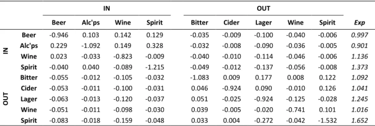
Table 10: Complete uncompensated price and expenditure elasticity matrix for alcoholic drinks.
IN OUT
Beer Alc'ps Wine Spirit Bitter Cider Lager Wine Spirit Exp
IN Beer -0.946 0.103 0.142 0.129 -0.035 -0.009 -0.100 -0.040 -0.006 0.997 Alc'ps 0.229 -1.092 0.149 0.328 -0.032 -0.008 -0.090 -0.036 -0.005 0.901 Wine 0.023 -0.033 -0.823 -0.009 -0.040 -0.010 -0.114 -0.046 -0.006 1.136 Spirit -0.040 0.040 -0.089 -1.215 -0.049 -0.012 -0.137 -0.056 -0.008 1.373 O U T Bitter -0.055 -0.012 -0.105 -0.032 -1.083 0.009 0.177 0.008 0.122 1.092 Cider -0.053 -0.011 -0.100 -0.031 0.046 -0.924 0.090 -0.010 0.126 1.041 Lager -0.063 -0.013 -0.120 -0.037 0.051 -0.025 -0.924 -0.125 -0.028 1.245 Wine -0.051 -0.011 -0.098 -0.030 0.039 -0.005 -0.020 -0.741 0.101 1.016 Spirit -0.083 -0.018 -0.159 -0.048 0.033 0.004 -0.272 -0.042 -1.532 1.652
The elasticity matrix for both sets of alcoholic drinks, those consumed at home (in) and those consumed away (out), is presented in Table 9, while the full elasticity matrix for alcoholic drinks is given in Table 10. Equivalent matrices have also been produced for each individual socio-demographic group in the sample, in order to investigate the impact of the policy on each group. In the majority of cases the drinks are own-price inelastic, the exceptions being alcopops and spirits at home and spirits away from home. Within the two groups (consumption at and away from home) there is a high degree of substitutability with the majority of cross-price elasticities being positive. A slightly different picture emerges when considering the effects between these groups where there is a high degree of complementarity although the magnitude of these effects is small. This complementarity is likely to arise largely as a result of the income effect of a price change in one group on the expenditure on drinks in the other group.
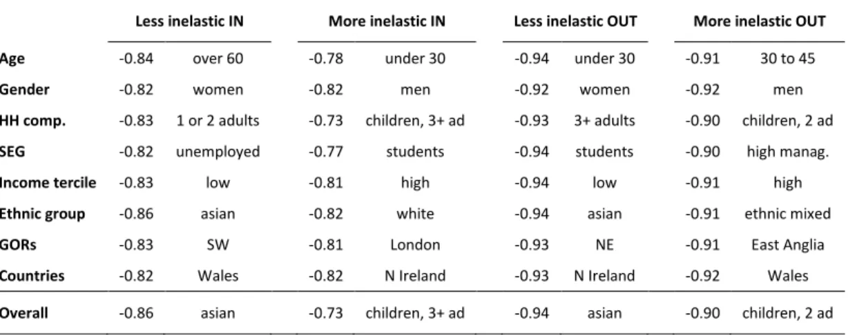
In the case of socio-demographic groups, there is somehow little variation in behaviour from the more responsive and less responsive categories. As seen in Table 11, own-price elasticities for drinking out are contained within the range -0.90 and -0.94, with the most inelastic being high managerial and high income; regarding consumption at home, the least elastic are households with 3 or more adults, student, and under 30. As for groups who are more elastic to price, at home it concerns mostly asian and over 60, while outside of home it concerns mostly asian, low income and under 30.
Table 11: Elastic and inelastic price response according to socio-demographic groups (uncompensated own-price elasticities).
Less inelastic IN More inelastic IN Less inelastic OUT More inelastic OUT Age -0.84 over 60 -0.78 under 30 -0.94 under 30 -0.91 30 to 45
Gender -0.82 women -0.82 men -0.92 women -0.92 men
HH comp. -0.83 1 or 2 adults -0.73 children, 3+ ad -0.93 3+ adults -0.90 children, 2 ad
SEG -0.82 unemployed -0.77 students -0.94 students -0.90 high manag.
Income tercile -0.83 low -0.81 high -0.94 low -0.91 high
Ethnic group -0.86 asian -0.82 white -0.94 asian -0.91 ethnic mixed
GORs -0.83 SW -0.81 London -0.93 NE -0.91 East Anglia
Countries -0.82 Wales -0.82 N Ireland -0.93 N Ireland -0.92 Wales
Overall -0.86 asian -0.73 children, 3+ ad -0.94 asian -0.90 children, 2 ad
4.3.
Impact on consumption
Corrected elasticities and price increases based on a minimum unit price of 50 pence have been used to determine the changes in quantities consumed, and results are presented in Table 12. Quantities purchased would decrease by an overall 14.8% as a result of a minimum price policy, with home consumption expected to decrease by just under 20%, and outside of home by just over 4%. The main drinks affected would be spirits consumed at home (-60.6%), and the least affected would be beer at home and wine and cider outside of home (all at -3.5%). However, consumption of some drinks is seen to increase for some specific socio-demographic groups, as a result of substitution between categories: home consumption of beer in London and of alcopops in Northern Ireland would actually increase (+6.5% and +12.7% respectively).
Table 12: Expected changes in units consumed according to alcohol groups.
Mean Highest decrease Lowest decrease
IN
Beer -3.5% -9.5% E Midlands 6.5% London
Alcopops -22.6% -66.6% North East 12.7% N Ireland
Wine -7.6% -34.5% unemployed -0.9% London
Spirit -60.6% -101.3% unemployed -25.0% students
O
U
T
Bitter -3.7% -7.4% unemployed -1.1% London
Cider -3.6% -7.3% unemployed -1.0% London
Lager -4.3% -8.1% unemployed -1.2% London
Wine -3.5% -6.8% unemployed -1.0% London
Spirit -5.7% -9.7% North East -1.7% London
In home -19.8% -38.0% unemployed -8.3% London
Outside -4.1% -7.8% unemployed -1.2% London
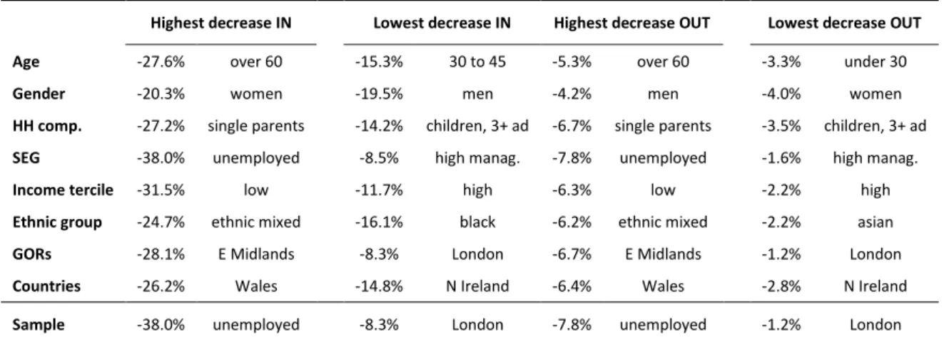
Table 13: Expected quantity (unit) changes according to socio-demographic groups.
Highest decrease IN Lowest decrease IN Highest decrease OUT Lowest decrease OUT Age -27.6% over 60 -15.3% 30 to 45 -5.3% over 60 -3.3% under 30
Gender -20.3% women -19.5% men -4.2% men -4.0% women
HH comp. -27.2% single parents -14.2% children, 3+ ad -6.7% single parents -3.5% children, 3+ ad
SEG -38.0% unemployed -8.5% high manag. -7.8% unemployed -1.6% high manag.
Income tercile -31.5% low -11.7% high -6.3% low -2.2% high
Ethnic group -24.7% ethnic mixed -16.1% black -6.2% ethnic mixed -2.2% asian
GORs -28.1% E Midlands -8.3% London -6.7% E Midlands -1.2% London
Countries -26.2% Wales -14.8% N Ireland -6.4% Wales -2.8% N Ireland
Sample -38.0% unemployed -8.3% London -7.8% unemployed -1.2% London
Table 13 summarises expected changes according to socio-demographic groups. Extreme changes (that is either maximum or minimum decrease in consumption) are observed for the unemployed who would see their intake decrease by 38.0% at home and 7.8% outside, and for Londoners who would see minimum changes in their intake (-8.3% at home, -1.2% outside). These contrasted effects of the price increase can be explained by several reasons: firstly, unemployed consume more at home than outside, and are therefore more exposed to the price increase; secondly, they tend to buy cheaper products, which means that the minimum pricing will result in a higher price increase for them; and thirdly, they have more elastic own-price and expenditures elasticities, resulting in a larger impact of the policy.
This can also be appreciated when considering absolute number of units consumed: unemployed would go from 22.5 units per week down to 15.9, while Londoners would decrease their intake from 29.8 down to 28.1. More generally, higher socio-economic groups and high income households, who are the main consumers of alcohol, would be the least affected while groups who currently consume smaller amounts of alcohol would be more severely affected.
4.4.
Impact on Expenditures
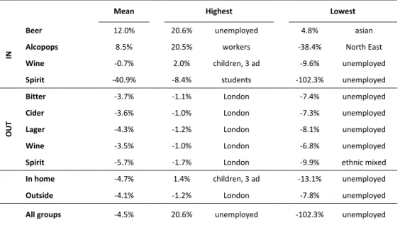
Table 14 reports the effects of a minimum price on expenditure. Total sales of alcohol would contract by 4.5%, with a 4.7% decrease for the value of sales at home, and 4.1% decrease for sales outside of home, even though pubs and restaurants would not be directly affected by the price rise, as their retail prices are already above the proposed threshold. Drinks consumed outside would all be affected in a similar way, with changes in expenditure ranging from -3.5% for wine, to -5.7% for spirits. The value of sales for home consumption would be differently affected according to the drinks considered: sales of beer and alcopops would actually increase in value (12.0% and 8.5% respectively) both in reason of their respective price increase and of a substitution effect from other drinks. Sales of spirits would decrease by over 40%; sales of wine would remain largely unaffected (contraction under 1%).
Table 14: Expected changes in alcohol expenditures according to alcohol groups.
Mean Highest Lowest
IN
Beer 12.0% 20.6% unemployed 4.8% asian
Alcopops 8.5% 20.5% workers -38.4% North East
Wine -0.7% 2.0% children, 3 ad -9.6% unemployed
Spirit -40.9% -8.4% students -102.3% unemployed
O
U
T
Bitter -3.7% -1.1% London -7.4% unemployed
Cider -3.6% -1.0% London -7.3% unemployed
Lager -4.3% -1.2% London -8.1% unemployed
Wine -3.5% -1.0% London -6.8% unemployed
Spirit -5.7% -1.7% London -9.9% ethnic mixed
In home -4.7% 1.4% children, 3 ad -13.1% unemployed
Outside -4.1% -1.2% London -7.8% unemployed
5.
Discussion & Conclusions
Our results indicate that a minimum price of 50ppu would entail a significant decrease in alcohol consumption. Only off-licence retailers would have to implement a price increase, as leisure venues are found to already operate over this threshold; as a result, and in spite of a slight move towards home consumption, pubs and restaurants would not be greatly affected by the overall predicted decrease in alcohol consumption.
The impact of the minimum price would be partly offset by a shift of expenditures from food products towards alcoholic drinks. Furthermore, while higher income households are found to be heavier drinkers than their less affluent counterparts, the price rise would not affect them as much, as they tend to consume more expensive drinks which are already above the price floor. As a direct consequence, wealthy households are the least likely to decrease their consumptions and to change their habits. So, while the scheme appears efficient as a blunt instrument aiming at decreasing general alcohol consumption, it might prove ill-fitted to address alcohol abuse among certain categories of the population. It remains also to be seen whether observed prices are an indicator of quality, and whether the latter affects nefarious effects of alcohol: has a cheap unit of alcohol the same health consequences as a more expensive one?
From the point of view of the public, whether pubs & restaurants would welcome the measure as a way to level out the competitive advantage of supermarkets is unclear, as they are set to lose from the scheme. Another point of contention concerns the implementation of the scheme, whether it should be considered as a floor price implemented by producers or retailers, or as a tax collected by retailers, and what should become of the extra revenue generated.
Our study has its limitations. Dealing with household data, it is not possible to assess consumption at the person level, and for instance to determine the number of teetotallers or underage drinkers in one particular household. Furthermore, expenditures are recorded over a 2-week period, and cannot precisely reflect actual consumption. For instance, and as noted in the DH/NHS guidelines, “saving up” 21 units over a week to binge on a Friday evening is more harmful than to consume 3 daily units. In that respect, and for the same consumption level between 2 households, all else being equal, it is not possible to differentiate between risky and safe behaviours.
6.
References
Blundell, R., and C. Meghir (1987) “Bivariate alternatives to the Tobit model.” Journal of Econometrics 34(1-2):179—200.
Booth, A., A. Brennan, P.S. Meier, D.T. O’Reilly, R. Purshouse, T. Stockwell, A. Sutton, K.B. Taylor, A. Wilkinson, and R. Wong (2008) The independent review of the effects of alcohol pricing and promotion. School of Health and Related Research, University of Sheffield, UK.
http://www.dh.gov.uk/prod_consum_dh/groups/dh_digitalassets/documents/digitalasset/dh_091383.pdf
DCMS (2008) Evaluation of the impact of the Licensing Act 2003. London: Department for Culture, Media and Sport. http://www.culture.gov.uk/images/publications/Licensingevaluation.pdf
Deaton, A., and J. Muellbauer (1980a) “An almost ideal demand system.” American Economic Review 70(3):312—326.
Deaton, A., and J. Muellbauer (1980b) Economics and consumer behavior. Cambridge: Cambridge University Press.
DH (2008) 150 Years of the Annual Report of the Chief Medical Officer on the State of Public Health. London: Department of Health.
http://www.dh.gov.uk/prod_consum_dh/groups/dh_digitalassets/documents/digitalasset/dh_096231.pdf
DH (2009) Alcohol advice, Public health improvement. London: Department of Health, retrieved February 2010. http://www.dh.gov.uk/en/Publichealth/Healthimprovement/Alcoholmisuse/DH_085385
Edgerton, D.L. (1997) “Weak separability and the estimation of elasticities in multistage demand systems.” American Journal of Agricultural Economics 79(1):62—79.
Leon, D.A., and J. McCambridge (2006a) “Liver cirrhosis mortality rates in Britain from 1950 to 2002: an analysis of routine data.” The Lancet 367(9504):52—56.
Leon, D.A., and J. McCambridge (2006b) “Liver cirrhosis mortality rates in Britain, 1950 to 2002.” Correspondence, The Lancet 367(9511):645.
NHS (2010) NHS advice on drinking limits. London: National Health Service, retrieved February 2010.
http://www.drinking.nhs.uk/questions/recommended-levels/
Norfolk, A. (2007a) “Drink limits ‘useless’.” The Times, Times Online, October 20, 2007.
http://www.timesonline.co.uk/tol/life_and_style/food_and_drink/article2697975.ece
Norfolk, A. (2007b) “How ‘safe drinking’ experts let a bottle or two go to their heads.” The Times,
Times Online, October 20, 2007. http://www.timesonline.co.uk/tol/life_and_style/food_and_drink/article2697975.ece ONS (2010) Alcohol-related deaths in the United Kingdom, 1991-2008. Statistical Bulletin. Newport:
Office for National Statistics. http://www.statistics.gov.uk/pdfdir/alc0110.pdf
ONS-NHS (2007) Statistics on alcohol: England, 2007. Statistical bulletin, The Information Centre.
Tiffin, R. and M. Arnoult (2008) “Bayesian estimation o the infrequency of purchase model with an application to food demand in the UK.” Working paper. http://mpra.ub.uni-muenchen.de/18836/
WHO (2000) International guide for monitoring alcohol consumption and related harm. World Health Organization, document WHO/MSD/MSB/00.4. Geneva: WHO.
http://whqlibdoc.who.int/HQ/2000/WHO_MSD_MSB_00.4.pdf
WHO (2010) Global Information System on Alcohol and Health (GISAH). World Health Organization database. Geneva: WHO. http://apps.who.int/globalatlas/dataQuery/default.asp