Performance analysis of robust stable PID controllers using dominant pole placement for SOPTD process models

(1)

Performance Analysis of Robust Stable PID Controllers Using

Dominant Pole Placement for SOPTD Process Models

Saptarshi Das1_{, Kaushik Halder}2_{, and Amitava Gupta}2

1) Department of Mathematics, College of Engineering, Mathematics and Physical Sciences, University of Exeter, Penryn Campus, Penryn TR10 9FE, United Kingdom

2) Department of Power Engineering, Jadavpur University, Salt Lake Campus, LB-8, Sector 3, Kolkata-700098, India

Author’s Emails:

[email protected], [email protected] (S. Das*)

[email protected] (K. Halder)

[email protected] (A. Gupta)

Phone number: +44-7448572598

Abstract:

This paper derives new formulations for designing dominant pole placement based proportional-integral-derivative (PID) controllers to handle second order processes with time delays (SOPTD). Previously, similar attempts have been made for pole placement in delay-free systems. The presence of the time delay term manifests itself as a higher order system with variable number of interlaced poles and zeros upon Pade approximation, which makes it difficult to achieve precise pole placement control. We here report the analytical expressions to constrain the closed loop dominant and non-dominant poles at the desired locations in the complex s-plane, using a third order Pade approximation for the delay term. However, invariance of the closed loop performance with different time delay approximation has also been verified using increasing order of Pade, representing a closed to reality higher order delay dynamics. The choice of the nature of non-dominant poles e.g. all being complex, real or a combination of them modifies the characteristic equation and influences the achievable stability regions. The effect of different types of non-dominant poles and the corresponding stability regions are obtained for nine test-bench processes indicating different levels of open-loop damping and lag to delay ratio. Next, we investigate which expression yields a wider stability region in the design parameter space by using Monte Carlo simulations while uniformly sampling a chosen design parameter space. The accepted data-points from the stabilizing region in the design parameter space can then be mapped on to the PID controller parameter space, relating these two sets of parameters. The widest stability region is then used to find out the most robust solution which are investigated using an unsupervised data clustering algorithm yielding the optimal centroid location of the arbitrary shaped stability regions. Various time and frequency domain control performance parameters are investigated next, as well as their deviations with uncertain process parameters, using thousands of Monte Carlo simulations, around the robust stable solution for each of the nine test-bench processes. We also report, PID controller tuning rules for the robust stable solutions using the test-bench processes while also providing computational complexity analysis of the algorithm and carry out hypothesis testing for the distribution of sampled data-points for different classes of process dynamics and non-dominant pole types.

Keywords:

dominant pole placement, PID controller tuning, second order plus time delay (SOPTD), control performance, robust stable controller, stability region, signal/system norms, gain/phase margin

(2)

Nomenclature:

m: Non-dominance parameter for pole placement, K : Open loop process DC gain,

L : Open loop process time delay,

T: Open loop process time constant or lag, 1

ol T

  : Open loop process natural frequency,

ol

 : Open loop process damping ratio,

cl

 : Closed loop process natural frequency,

cl

 : Closed loop process damping ratio,

p K : Proportional gain, i K : Integral gain, d K : Derivative gain, s : Laplace operator, 2    : System norms, 2    : Signal norms, m G : Gain margin, m  : Phase margin, gc

 : Gain crossover frequency, d(t): Disturbance input,

u(t): Control signal, y(t): output variable, e(t): control error signal, J: Performance measure,

 

e

S s : sensitivity function,

 

T s : complementary sensitivity function,

 

d

S s : disturbance sensitivity function,

 

u

S s : control sensitivity function 1. Introduction

(3)

The dynamic behaviours of many industrial processes are affected and governed by significant amount of time delays in the control loops. The time delay is caused by the flow of information, energy and transport of physical variables, computer processing time etc. (Normey-Rico & Camacho 2007). The introduction of the time delay makes the continuous time closed loop system to have an infinite order (Åstrӧm & Wittenmark 2011) upon exponential series expansion of the delay term (

Ls

e _{) which is difficult to handle with a finite term controller (Michiels et al. 2002). To alleviate this}

problem, there have been several works to design controllers for such systems e.g. in (Zhong 2006). It is well known that most of the controllers used in the process industries are of PID type (Ǻstrӧm & Hägglund 1995) (Zhong 2006) due to its simplicity and ease of implementation, nice disturbance rejection, tracking performance etc. Amongst many other available approaches, the Internal Model Control (IMC) based tuning of PID controllers has been quite popular to handle First Order Plus Time Delay (FOPTD) and Second Order Plus Time Delay (SOPTD) processes, as well as Integral Process with Dead Time (IPDT) (Shamsuzzoha & Lee 2007; Rivera et al. 1986) because of its good robustness on uncertain plants. Another approach on the design of smith predictor augmented PID controller to handle time delay processes have been reported in (Astrom et al. 1994) which yields improved tracking and load disturbance rejection performances. A modified methodology is proposed with combined Smith predictor and PID controller in (Matausek & Micic 1996) considering challenging higher order integrating plants with delays. However the main drawback of this method is that it cannot handle unstable process with delay (Normey-Rico & Camacho 2007), unless an additional observer is used (Furukawa & Shimemura 1983). To overcome these problems of complicated time delay processes, the model predictive control (MPC) has got attention by many researchers but there are only few results for time delay systems (Ellis & Christofides 2015). Initially the MPC was developed mainly to control slower processes as it requires large computational burden for prediction and optimisation-based control. MPC controller design for time delay systems is mostly an open area and there are only few results like (Holis & Bobál 2015). Another important area is designing output feedback controller (De la Sen 2005) as well as state feedback controller (Michiels et al. 2010) for stabilizing time delayed systems which are gradually gaining increased attention. In the literature some control algorithms are proposed using linear matrix inequalities (LMIs) for time delayed systems e.g. (Niculescu 1998) to enforce robustness and several closed loop performance measures. Despite having these results, traditional pole placement remained quite challenging for time delay systems because of its increased or even infinite order.

In this paper, we propose an analytical formulation for dominant pole placement tuning of PID controllers to handle SOPTD systems. This is due to the fact that in many process industries, the dynamical behaviours in a large variety of self-regulating processes can be modelled using the SOPTD template with the flexibility of showing both sluggish and oscillatory open loop dynamics as well as different lag to delay ratio or normalized dead time (O’Dwyer 2009). PID controllers are traditionally tuned by various means like time and frequency domain performance criteria or design specifications (Cominos & Munro 2002). Amongst many available approaches, the dominant pole placement method has been quite promising as the designer can specify his demand of closed loop performance, as the equivalent second order system’s damping ratio, time constant or natural frequency (Wang et al. 2009). Amongst previous approaches, dominant pole placement based PID controller design for delay free second order systems have been addressed in (Saha et al. 2012)(Das, Halder, et al. 2012) whereas its time delay version has been extended in this paper and the method has been verified on several test-bench SOPTD plants.

A continuous pole placement method (controlling the rightmost root of the closed loop system and shift it to the left half of the s-plane in quasi-continuous way) has been proposed to design a semi-automated pole placement based state feedback controller for retarded (Michiels et al. 2002) and neutral type (Michiels & Vyhlidal 2005) delay systems. By this method, the closed loop roots lying in the extreme right-hand side is shifted to the far possible left-hand side. However, the methodology

(4)

does not allow direct pole placement for SOPTD system and only monitoring the real part of the roots. To overcome the above problem another methodology is proposed in (Michiels et al. 2010) which combines direct pole placement and the minimization of the spectral abscissa for determining controller parameters in retarded time-delay systems. There are some other approaches on stability analysis of time delayed single input single output (SISO) systems to derive controller gains by computing the root locus. Using the characteristic equation which leads to a transcendental equation in the presence of delays which is also known as the quasi-polynomial, several methods have been proposed to construct the root locus which creates horizontal asymptotes (Krall 1970; Yeung & Wong 1982; Huang & Li 1967). Other root locus based stabilization methods are also reported to analyse state space models with input delay (Engelborghs et al. 2001), state delay or both (Suh & Bien 1982) by using the root locus.

The PID controller tuning by direct pole assignment is found to be a difficult approach for time delay systems, as the time delay in a process makes the closed loop system to have an infinite order. Therefore, to handle time delay systems, the direct pole placement in complex s-plane is not recommended as suggested in the pioneering work on dominant pole placement tuning in (Wang et al. 2009). The methodology in (Wang et al. 2009) also suggested a Nyquist based design for frequency domain stabilization of the time delay systems using PID controllers. The main hurdle with the pole placement for delay systems has been the fact that the exponential delay term in Laplace domain (i.e.

Ls

e _{), manifests itself as very high order transfer function upon approximations using Pade/Routh}

methods of a specified order (Silva et al. 2007). Therefore, such a pole placement approach will need relocation of many open loop poles at a time with a compact finite term (three-term for PID) controller when the number of interlacing pole-zeroes, arising due to the approximation of the time delay term are too many to handle for a chosen order of approximation. In our derivations, the order and approximation method are considered to be fixed. In particular, we apply a third order Pade approach to approximate the time delay term in the process model. Therefore, it can be considered as a new area of research to get a clearer picture of the dominant pole placement design for time delay systems where the task is to handle many poles and zeros of the combined plant and delay with finite number of controller parameters. To demonstrate the methodology, SOPTD processes with various delay to lag ratio have been used which shows the strength of the algorithm for even quite challenging plants e.g. delay dominant systems with low open loop damping which are much harder to control using standard PID controller tuning methods.

2. Theoretical formulation

In this section, the dominant pole placement based PID controller design has been shown to handle SOPTD systems. The time delay term has been approximated using a third order Pade’s approximation instead of considering it as transcendental term in the quasi-polynomial (Silva et al. 2007). The co-efficient matching based pole placement method has been described previously in (Ǻstrӧm & Hägglund 1995)(Kiong et al. 1999) for the control of delay free systems. We apply here a similar co-efficient matching method to design dominant pole placement based PID controller gains using the characteristic equation having third order Pade approximation of the delay term.

Now, let us consider the open loop SOPTD process can be represented by:

2 2 ( ) 2 Ls ol ol ol K G s e s   s      , (1)

which is to be controlled by the PID controller 2 ( ) i d p i p d K s K s K K C s K K s s s       . (2)

(5)

Then the closed loop system with PID controller can be written as:

 

   

_{   }

1 cl G s C s G s G s C s   . (3)

Again, using a third order Pade approximation for the time delay term (

e

Ls) of the open loop SOPTD process model (1) can be written as:

3 3 2 2 3 3 2 2 12 60 120 12 60 120 Ls L s L s Ls e L s L s Ls  _       . (4)

Therefore, the full expression of the closed loop system transfer function including the open loop plant and PID controller is given by:











 





2 3 3 2 2 2 2 3 3 2 2 2 3 3 2 2 12 60 120 2 12 60 120 12 60 120 d p i cl ol ol ol d p i K K s K s K L s L s Ls G s s   s  L s L s Ls K K s K s K L s L s Ls                    . (5) It is evident from (5) that the closed loop process has six poles and five zeros which can be modulated using suitable choice of the three controller gains



K K K_p, ,_i _d



. As the closed loop system in (5) has six poles, the corresponding desired closed-loop characteristic polynomial should also contain six roots out of which two must meet the equivalent desired closed loop system specifications. Rest of the four non-dominant poles can be allowed to have different characteristics e.g. all four complex conjugate poles, all four real poles, two real and two complex conjugate poles which have been described in the following sub-sections along with the respective derivations for the dominant pole placement tuning.

2.1. Deriving unique and alternative expressions for stabilizing PID controller gains and obtaining the stability regions

Using the coefficient matching of the desired vs. the given characteristic equation of the closed loop system, we show here that for a chosen set of process parameters



K L T, , ,



ol



, the expressions for integro-differential gains Ki and Kd produce unique values. But there can be many alternative expressions for the proportional gain Kp which can be derived from the two controller gains Ki and Kd. The multiple expressions for Kp arise due to an overdetermined system of algebraic equations from various higher powers of the Laplace variable s. Therefore, for a given set of plant parameters and design specifications, after obtaining the controller gains



K Ki, d



, there can be many possible solutions for Kp. The most robust expression for selecting Kp can be found out by comparing the stabilizing regions for all these expressions having the highest volume, compared to the same with the others. This is determined by drawing uniformly distributed random samples from a chosen design parameter space with a specified range and then evaluating the stability at each of these sampled points, as determined by the real part of the closed loop poles being negative.

In order to show this, we use Monte Carlo simulations by sampling the design specifications



m,

 

cl, cl



from chosen intervals for fixed open loop plant parameters



 

ol, ol,L



. The effect of system’s DC-gain K has not been investigated here, since it simply decreases all the three PID controller gains in a linear fashion. However, the effect of other parameters may be complicated and therefore needs to be explored rigorously using Monte Carlo simulations which is adopted next.

(6)

Let us now assume that for a given set of open loop plant parameters



 

ol, ol,L



, one can choose

different design specifications



m,

 

_cl, _cl



to derive the PID controller gains. However, due to the finite term approximation of the time delay, the resulting closed loop system is not necessarily stable for any randomly chosen design parameter or arbitrary PID controller gains within a specified range. We substantiate this argument, using a computational approach of randomly sampling the design specification space within a chosen bound, for fixed open loop SOPTD process parameters which yields a set of stabilizing PID controller gains



K K K_p, ,_i _d



. However, with different design specifications



m,

 

cl, cl



, the closed loop system may be stable, but the closed loop performance is expected to vary widely within this entire stability region. Such thousands of randomly sampled guess values for the design specifications yielding stable closed loop systems can be quantified as a fraction of the accepted stable samples to the total number of samples drawn from the entire design specification space. For a more robust system design, the method producing largest stabilizing volume in the design parameter space or the equivalent controller parameter space should be selected.

For the set of stabilizing controller gains, we also calculate various closed loop performance measures like set-point tracking, disturbance rejection, control effort to investigate their trade-offs (Das & Pan 2014), peak sensitivity and complementary sensitivity functions etc. (Åstrӧm & Hägglund 2004) signifying parametric robustness and high frequency measurement noise rejection performances respectively. We also demonstrate here the wide applicability of our proposed approach on three different class of SOPTD processes e.g. lag-dominant (

T L



), delay dominant (

T L



) and balanced lag-delay (

T L



) system, also each of them with three different damping levels viz. overdamped (

1

ol



 ), critically damped (



_ol 1), and underdamped (



_ol 1). Therefore, we have nine different cases to explore, as shown in the subsequent sections. For the Monte Carlo simulations, the ranges for the desired control performance parameters are chosen as m

 

1,10 ,



_cl 

 

1,5 ,



_cl

 

1,10 , as per the previous reports like (Panda et al. 2004)(Wang et al. 2009).

2.2. Pole placement PID controller design with all non-dominant complex conjugate poles Now, as discussed in (Kiong et al. 1999)(Ǻstrӧm & Hägglund 1995) in order to ensure guaranteed dominant pole placement with PID controllers, let us consider that the closed loop system (5) has six complex (conjugate) poles. Amongst these six, two of them are dominant meeting the desired closed loop design specifications



 

cl, cl



. The rest four poles are non-dominant in nature and their locations can be controlled by selecting the non-dominance pole placement parameter m. One can easily choose the m in such a way that these poles do not have any significant effect on the closed loop performance of the process with design specifications



 _cl, _cl



. Under this assumption, the non-dominant closed loop complex conjugate poles become



2



1,2 1

nd

cl cl cl cl

s m    j  . Therefore, the resulting characteristic polynomial with both dominant and non-dominant poles can be written as:









 





























4 2 2 2 2 2 1 2 2 2 2 2 1 2 1 2 2 2 2 2 2 2 2 2 2 2 2 2 2 2 2 2 ( ) 2 2 2 2 2 1 2 2 0. nd cl cl cl nd nd cl cl cl nd nd nd nd cl cl cl cl cl cl cl cl cl cl cl cl cl cl cl cl cl cl s s s s s s s s s s s s s s s s s s s s s m s m m s s s m s m                                                      (6)

(7)

characteristic polynomial (6) can be expanded in terms of the open loop process parameters and the PID controller gains as:

6 3 5 2 3 3 4 2 2 3 2 3 3 2 2 2 3 2 2 2 1 2 12 2 60 24 12 120 120 12 60 12 240 60 120 60 12 120 120 60 ol ol d ol ol ol d p ol ol ol d p i ol ol ol d p i ol P i s L s L L KK L s L L L KK L KK L s L L KK L KK L KK L s L KK KK L KK L s KK KK L                    _   _    _     _    _      _    _     _   _  





0 ₁₂₀ 0. i s KK    (7)

Now the characteristic polynomial in terms of the desired closed loop poles in (6) can also be written as:

 

















6 5 4 2 2 2 2 2 2 3 3 3 2 3 2 3 2 4 4 3 2 4 2 4 2 1 4 5 3 5 0 4 6 1 4 2 2 1 2 8 4 4 1 2 4 8 2 1 2 2 4 0. cl cl cl cl cl cl cl cl cl cl cl cl cl cl cl cl cl cl cl cl cl cl cl cl cl cl s s m s m m s m m m s m m m s m m s m                                _    _    _    _    _    _    _  _       (8)

For comparing the coefficients of these two characteristic polynomials, after dividing (7) by_L3_and

comparing it with (8), the corresponding PID controller gains can be easily obtained as:













2 4 4 3 2 4 2 2 3 2 3 4 6 3 0 5 1 3 5 3 4 6 4 2 2 2 4 3 3 3 : 120 12 : 2 2 1 2 : 4 2 240 240 240 60 120 12 ₈ ₂ _{1 2} ₆₀ 4 : : cl i d ol ol cl cl p cl cl cl ol o ol ol l d p i cl cl cl cl cl c p m L s K K s K m K L s K m L m m L K s L KK KK m m m K L L L L s K m K L    _ _{ }                _    _                         

















2 2 2 3 2 4 2 2 3 2 3 3 2 2 2 2 2 2 4 1 2 4 120 120 12 60 12 24 12 60 : 2 1 2 8 . cl ol ol ol d i ol ol d p ol cl cl cl c l cl cl cl cl cl l cl m m L L KK L KK L KL KK s K m m K L L L                   _ _ _ _ _ _ _      _        _    (9)

It is observed from (9) that the expressions for the two PID controller gains



K K_i, _d



are unique but the proportional gainK_pcan have four possible expressions.

(8)

Similar to the above closed-loop characteristic equation in order to find the PID controller gains, the non-dominant poles can also be considered as real (instead of imaginary) and still be manipulated by the non-dominance pole placement parameter m while meeting the same dominant closed loop specification



 _cl, _cl



. Therefore, for all real non-dominant poles, the characteristic equation becomes:















4 2 2 2 2 4 3 2 2 2 2 3 3 3 4 4 4 ( ) 2 2 4 6 4 0. cl cl cl cl cl cl cl cl cl cl cl cl cl cl cl cl s s s s m s s s m s m s m s m                              (10)

The desired characteristic polynomial (10) can be expanded and rearranged according to the power of Laplace variable s, as required for the coefficient matching with that of the open loop system with PID controller in (7), which yields:

 





6 5 4 2 2 2 2 2 2 3 3 3 3 2 3 3 3 2 4 4 4 3 4 4 2 2 4 1 4 5 5 3 3 5 0 4 4 6 1 4 2 6 8 4 12 4 8 6 2 4 0. cl cl cl cl cl cl cl cl cl cl cl cl cl cl cl cl cl cl cl cl cl cl cl cl cl cl cl s s m s m m s m m m s m m m s m m s m                                 _   _    _   _    _   _    _  _       (11)

Now in a similar way dividing (7) by_L3_{and matching the coefficients of}_s_{with (11) yields the}

corresponding PID controller gains for the real non-dominant poles as:









2 4 4 3 4 4 2 2 3 2 3 0 4 4 6 3 5 1 3 4 5 5 3 3 5 2 2 2 240 60 120 12 4 ₈ 4 : 120 12 : 2 2 1 2 : 2 4 120 60 120 : 6 60 i cl cl d ol ol cl cl p cl cl cl cl ol i ol p ol ol d i cl cl cl cl cl cl s K m L K s K m K L s K L m m K KK KK L m m m K L K s K K L L L L            _ _{ } _                           _    _     



 



3 3 3 2 2 2 3 2 4 2 2 2 3 3 2 3 3 2 2 2 4 2 2 2 : 4 4 120 120 12 60 12 24 12 60 : 6 8 . 12 p ol ol ol d i ol ol d p ol cl cl cl c cl l cl c cl c l l l c cl s K L m m m L L KK L KK L KL KK s K m m K L L L      _ _{ } _           _      _   _       _     . (12) Here also, the two PID controller gains



K K_i, _d



can be uniquely derived from the open loop and desired process parameters, but the proportional gain Kp can have four different expressions.

2.4. Pole placement PID controller design with two real and two complex conjugate non-dominant poles

The characteristic equation using two real and two complex conjugate non-dominant poles can be written as:



2 2



2 2 2







2

( )s s 2 cl cls cl s 2m cl cls mcl s m cl cl 0

(9)

 





6 5 4 2 2 2 2 2 2 2 4 3 3 3 3 3 3 2 3 3 2 3 3 2 3 3 2 4 2 4 3 4 4 3 2 4 2 2 4 2 2 4 2 1 4 2 5 8 2 2 2 8 2 4 4 4 4 cl cl cl cl cl cl cl cl cl cl cl cl cl cl cl cl cl cl cl cl cl cl cl cl cl cl cl cl cl cl cl cl s s m s m m m s m m m m m m s m m m m m m                                      _    _    _      _       4 1 4 3 5 3 3 5 3 5 0 4 2 6 2 2 2 0. cl cl cl cl cl cl cl cl cl s m m m s m                 _   _       (14)

Again, dividing (7) by_L3_{and match the co-efficient with (14) as done previously, yields the} corresponding PID controller gains as:









2 3 2 0 4 2 6 3 5 1 3 4 3 5 3 3 5 3 5 2 2 2 4 2 4 3 4 4 3 2 3 : 120 12 : 2 2 1 2 : 2 2 2 120 60 120 : 240 60 120 12 4 4 i cl cl d ol ol cl cl p cl cl cl cl cl cl ol i ol p ol ol d i cl cl cl cl cl c KK KK L L L s K m L K s K m K L s K L m m m KK L K s L L m m m K                      _    _    _                



 











4 2 2 4 2 2 4 2 4 3 3 3 3 3 2 3 3 2 3 3 2 3 3 3 3 2 2 2 3 4 2 2 60 : 12 120 120 12 4 2 2 2 60 24 8 2 12 60 : 4 5 l cl cl cl cl cl cl cl cl cl cl cl cl cl c p ol ol ol d i ol ol d p l cl cl ol cl K L s K KL L L KK L KK m m m m m L KK s K m m L L m m L                       _                                



2 2 2 2 2 ₈ 2 2 4



_. cl cl cl cl cl cl m  m m   K        (15)

Similar to the previous cases,



K Ki, d



gains have unique expressions but the gain Kphas four possible values depending on the choice of different coefficients of Laplace variable s.

3. Designing robust stable PID controller and evaluation of different closed loop performance measures

3.1. Determining the robust stable solutions using centroid of the stability region

We here use the k-means clustering algorithm to determine the centroid of the stability region in the PID controller space which can have a complex shape in the 3D parameter space of the controller gains



K K K_p, ,_i _d



. The stability regions are determined for nine classes of SOPTD plants and it is also checked that a single centroid represents the stability regions of a unimodal distribution in the controller parameter space. Otherwise if a multi-modal distribution is discovered, indicating more than one possible robust stable solution for the controller gains, the number of centroids (k) in the k -means clustering algorithm can also be set to the number of modes in the distribution of controller gains. Previously determination of the stability region centroids in the controller parameter space were done by looking for only circular (for two gains), spherical (for three gains) or (hyper)-spherical clusters (more than two controller gains) as shown in (Pan et al. 2011), which has been extended here to find out centroids of more generalised complicated shaped clusters like ellipsoids or other structures by assuming that the centroid is likely to lie in the high density region of the clusters where most of the samples are accepted in the random Monte Carlo sampling.

Although the chosen design parameter space has been explored using 105_{uniformly distributed}

(10)

has more stable solutions than the others. Therefore, the present random sampling approach helps in understanding the shape of the stability region using various expressions for deriving the PID controller gains, while also giving the flexibility to specify the nature of the non-dominant poles (i.e. all real, all complex or mixed), as explored in the previous sections.

The k-means clustering algorithm starts with a random initial guess for the centroid of the multi-dimensional data space and iteratively move the centroids based on minimizing the squared Euclidean distance criteria from all the data points (Rogers & Girolami 2012). However, to ensure that the best possible estimate of the centroid or the robust stable solution has been discovered in the iterative process, the k-means clustering has been run 10 times, for each case with random starting points and the best solution with minimum Euclidean distance is chosen as the final estimate of the centroid, signifying the most robust stable solution in the PID controller parameter space.

Therefore, for a given process model characterised by the constants



K,

 

_ol, _ol,L



, the robust stable PID controller gains obtained via the dominant pole placement can be obtained using the following steps:

Step 1: Choose the non-dominant pole types amongst all complex, all real or mixed using the expressions in (9), (12) or (15) to map the open loop and desired closed loop system parameters on to the PID controller gains.

Step 2: Obtain the stabilizing PID controller gains using few thousands of uniformly distributed samples within a chosen range of all design parameters



m,

 

cl, cl



.

Step 3: Cluster the stabilizing PID gains to get the centroid as the robust stable solution.

Step 4: Evaluate different performance measures with the robust stable PID controller on the nominal and perturbed process models.

3.2. Performance measures with the stabilizing PID controller gains

The previous section derives the expressions for obtaining stabilizing PID controller gains by choosing the nature of the non-dominant poles being all complex, real or mixture of them. However, in a realistic control system design problem, apart from the stability, the control loop performance is also of major concern. Therefore, the robust stable solutions might not always show an acceptable control performance. On contrary the controller setting for optimised performance criteria may not have a sufficient robustness against plant or controller parameter variation. Therefore, we chose to design the PID controller settings based on maximum robust stability and then compare the achievable control performances. However the robustness checking of optimally designed controllers is also a valid approach as previously studied for single control objective (Das, Pan, et al. 2012; Das et al. 2011) and multiple conflicting control objectives (Das et al. 2015)(Das & Pan 2014). Also, the parametric robustness of optimal controllers and optimality of robust design have been previously discussed in (Pan & Das 2016).

After the robust stable solution is determined using clustering which yields the centroid of the arbitrary shaped stability region, few well-known performance measures are calculated next to compare the effect of having different type of non-dominant poles. Amongst these, both time and frequency domain performance measures are evaluated, however both of them are neither specified nor can be guaranteed together, under the present design approach, as also shown in (Das et al. 2011). However for a fair comparison we evaluate different control performances with the PID controller gains obtained using different non-dominant pole types e.g. gain and phase margin (Gm and Φm) and gain crossover frequency (ωgc) controlling the overshoot vs. speed of operation (Das et al. 2011), peak sensitivity and complementary sensitivity (Ms and MT) (Åstrӧm & Hägglund 2004),  ₂ _norms for

(11)

tracking or command following mode (servo) and disturbance rejection (regulatory) mode (Alcántara et al. 2013)(Arrieta et al. 2010).

Let, G s_ol

 

be the open-loop transfer function comprising of the time-delayed SOPTD system

 

G s with PID controller C s

 

which can be represented as:

 

   

ol

G s C s G s . (16)

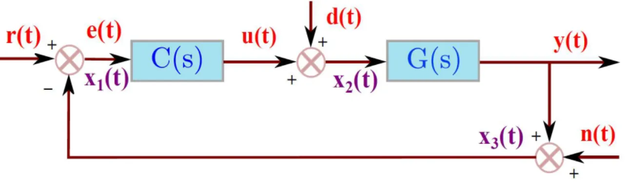
The basic PID control loop with different inputs e.g. set-point (r), disturbance (d) and noise (n) and the measurement points e.g. error (x1), control signal (x2) and noisy process variable (x3) are shown in Figure 1. To guarantee internal stability and also for evaluating different performance measures of a feedback control loop the following nine transfer functions in (17) play a major role (Doyle et al. 2013) 1 2 3 1 1 1 1 1 1 x e G r x u d C C d GC x y n GC G n             _ _ _  _        _                      . (17)

These matrix shows the effective transfer functions from different inputs to various measurement points. Amongst the nine, four transfer functions play the central role to characterise the control system performance (Doyle et al. 2013)(Das & Pan 2014)(Herreros et al. 2002), i.e. the sensitivity

 

e

S s , complementary sensitivity T s

 

, disturbance sensitivityS sd

 

and control sensitivityS su

 

as follows:

 

_{ }

 

_{ }

 

_{ }

 

_{ }

 

2 3 3 3 2 1 , 1 , 1, 1 , . 1 1 e re dx nx ol ol e rx ol d u dx rx ol ol S s G s G s G s G s G s T s G s S s T s G s G s C s S s G s S s G s G s G s                 (18)

These four transfer functions can be quantified using various systems norms ( ₂ _) for different system inputs (Herreros et al. 2002). It is clear from (18) that the sensitivity function S se

 

has three different interpretations. In other words, the sensitivity function signifies the effective transfer function at all the three measurement points in Figure 1, for set-point, disturbance and noise inputs, as also revealed from the same diagonal elements in (17). Therefore, in a process control design, it has been considered as one of the fundamentally important criteria which is often considered to be norm bounded in various tuning rules like MIGO (M-constrained integral gain optimization) and approximate MIGO (AMIGO) etc. for PI/PID controller design (Åstrӧm & Hägglund 2004; Hägglund & Åstrӧm 2004)(Hägglund & Åstrӧm 2002).

First we check the performance

 

Jd for a step disturbance input



d s

 



and calculating the

2 

  norms of the disturbance sensitivity function which can be represented by:

   

 

   

 

2 1 ₂ 1 2 2 , 1 , , 1 . d d d d J d s S s d s s J_ d s S s _ d s s     (19)

(12)

Using the final value theorem for Laplace transform, the functions with finite time domain integral are quantified and accordingly the set-point/disturbance inputs are selected between step/impulse as

 

r d, 1s or

 

r d, 1 respectively, as the input to different sensitivity functions.

Figure 1: Schematic diagram of the PID control loop with different inputs and measurement points.

The controller output or the control signal leads to the actuator limits and frequent oscillatory inputs to the actuator

J

u which can be represented by the  ₂ _ norms of the control sensitivity function. However, for standard PID controller structure without a derivative filter as being used here for obtaining 3 controller parameter based 3D stability regions, the control sensitivity becomes an improper transfer function with more zeros than poles which forbids calculating system norms directly. As an alternative approach, the  2  norms of the control signal can be computed for a

step input to u

 

S s if it is proper, or impulse input to u

 

S s s if the control sensitivity is improper, as in the present case. Therefore the control sensitivity norms can be quantified as the 2 norm for

step change in the set-point using inverse-Laplace transform (_1_{) of}_Su

_{ }

_{s s}_as:

 



   



 



   



 

1 2 ₂ 1 ₂ 1 1 2 2 , 1 , , 1 . u u u u u u J S t d s S s d s s J S t d s S s d s s    _ _         (20)

The set point tracking performance

J

eis analysed using the sensitivity function subjected to step change in the set-point yielding

   

 

   

 

2 1 ₂ 1 2 2 , 1 , , 1 . e e e e J d s S s d s s J d s S s _ d s s     (21)

The noise rejection performance can be quantified as

J

nusing the complementary sensitivity function subjected to impulse input in the set-point yielding

   

 

   

 

2 1 ₂ 1 2 2 , 1, , 1. n n J d s T s d s J_ d s T s _ d s     (22)

For all the different sensitivity functions, the corresponding ₂ _system norms and ₂ _signal norms are defined as:

(13)

 

2 2 2 2 1 , sup , 2 , sup . t G s G j d G s G j g t u t dt g t g t               



(23)

The₂norms here in (19), (21) and (22) represent large and sustained oscillations in the disturbance response, error signal and process variable, whereas thenorms denote the peak gain of the

frequency response for a particular type of input (servo/regulatory). For stable closed loop system, the corresponding 2 norms of the sensitivity functions with a chosen type of input excitation need to be

finite and should have a low-pass characteristic i.e. as , the Bode magnitude plot should be drooping in nature.

Next we also compute the gain margin (G_m), phase margin (_m) and the gain cross-over frequency (_gc) of the open loop system which signify the robustness, oscillatory nature and speed of the closed loop response respectively. These three important quantities for a given process model and set of PID controller gains can be derived as:







 









 









 









 



1 1 . ol gc gc gc m ol gc gc gc ol pc pc pc m ol pc pc pc Arg G j Arg C j G j G j C j G j G j C j G j G Arg G j Arg C j G j                                       (24)

4. Simulation and results

4.1. Test-bench SOPTD processes for performance evaluation

For each of the nine classes of test-bench plants under investigation, we also tabulate which pole configuration and expression for the PID controller gains yield the largest stability region, as explored from the number of stabilizing solutions obtained from the Monte Carlo simulations on the chosen design parameter space. The percentage volume can be represented as the ratio of accepted stable solutions to the total number of uniformly distributed (105_{) random samples drawn from the chosen}

parameter space. In addition, the correlation amongst the stabilizing controller gains or the design parameters are also investigated. For example, it can be observed that a high _cl can only be achieved with small m i.e. allowing more effect of the non-dominant poles, thus unnecessarily affecting the control performance. Similarly, an inverse relation is observed between the stabilizing _cl and _cl. In principle, a high value of m is desired which keeps the effect of non-dominant poles on the control performance as minimum. However it will be evident from the simulation examples presented later that the high m regions are sparse and is also limiting the design specification on the _cl and _cl.

The nine classes of test-bench processes and their characteristics are as follows: i) Lag-dominant (L<T) underdamped (ζol<1) process (Jahanmiri & Fallahi 1997)

1 2 1 ( ) 9 2.4 1 s G s e s s     , (25) with K = 1/9, L = 1, T = 3, ζol = 0.4, L/T = 0.333<1.

(14)

0.8 2 2 1 ( ) 2 1 s G s e s s     , (26) with K = 1, L = 0.8, T = 1, ζol = 1, L/T = 0.8<1.

iii) Lag-dominant (L<T) overdamped (ζol>1) process (Pomerleau et al. 1996)







2 3( ) 1 10 1 4 s e G s s s     , (27) with K = 1/40, L = 2, T = 6.3246, ζol = 1.1068, L/T = 0.3162<1.

iv) Balanced lag-delay (L≈T) underdamped (ζol<1) process (Hwang & others 1995)

4 2 0.5 ( ) 1.2 1 s G s e s s     , (28) with K = 0.5, L = 1, T = 1, ζol = 0.6, L/T = 1.

v) Balanced lag-delay (L≈T) critically-damped (ζol=1) process (Hägglund & Åstrӧm 2004)





5( ) 2 1 s e G s s    , (29) with K = 1, L = 1, T = 1, ζol = 1, L/T = 1.

vi) Balanced lag-delay (L≈T) overdamped (ζol>1) process (Panda et al. 2004)

3 6( ) ₉ 2 ₂₄ ₁ s e G s s s     , (30) with K = 1/9, L = 3, T = 3, ζol = 4, L/T = 1.

vii) Delay dominant (L>T) underdamped (ζol<1) process (Wang & Shao 2000)

1.2755 7( ) _3.2158 2 _3.1614 _3.0568 s e G s s s     , (31) with K = 1/3.2158, L = 1.2755, T = 1.0257, ζol = 0.5042, L/T = 1.2435>1.

This is a reduced order model of a highly oscillatory higher order process

 



2







1 1 3 s G s e s s s      .

viii) Delay dominant (L>T) critically-damped (ζol=1) process (Thyagarajan & Yu 2003)





10 8( ) 2 1 s e G s s    , (32) with K = 1, L = 10, T = 1, ζol = 1, L/T = 10>1.

ix) Delay dominant (L>T) overdamped (ζol>1) process (Bi et al. 2000)

2 9( ) _0.12 2 _1.33 _1.24 s e G s s s     , (33)

with K = 1/0.12, L = 2, T = 0.3111, ζol = 1.7239, L/T = 6.4288>1. This represents an HVAC system model between fan speed to the supply air pressure control loop.

(15)

The next sub-section reports the stability regions of each of these nine classes of test-bench processes, representing different dynamical behaviour with various lag to delay ratio and open loop oscillation levels.

4.2. Stability regions and the robust stable PID controller design for the test-bench SOPTD processes

Out of the 12 possible expressions (3 non-dominant pole types × 4 different coefficient orders of Laplace variable to find out Kp) for the stabilizing gains, we now identify the stabilizing data points within a range of design parameters for the expression where the number of stable solutions is maximum. The stabilizing data-points in the design parameter space



m,

 

_cl, _cl



are next projected on to the controller parameter space



K K K_p, ,_i _d



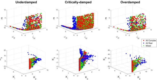
by an one to one mapping using the expressions in (9), (12) and(15). These sets of stabilizing controller gains are then fed to a clustering algorithm to find out the centroids of the stabilizing regions, for each of the non-dominant pole types. Next, the performances of these robust stable solutions are also compared, using various criteria introduced in section 3.2.

Figure 2: 3D stability region in the design specification and controller parameter space for the three lag-dominant processes. (top) design parameter space, (bottom) PID controller parameter space.

For the nine test-bench processes in (25)-(33), the stability regions in the design parameter space (top panels) and PID controller parameter space (bottom panels) are shown in Figure 2-Figure 4 respectively. Out of the 105_{uniformly drawn samples in the chosen design parameter space}



m,

 

cl, cl



, the number of stabilizing solutions are reported in Table 1 for the nine test-bench processes and different non-dominant pole types and expressions for proportional gain Kp. It is also evident from Table 1 that the all complex non-dominant pole type and the first (s1_{) expression for}_K_p,

yields a larger stabilizing region given by the percentage (%) volume or the number of stable solutions, obtained from the randomly drawn samples. This is due to the reason that for all four complex non-dominant poles, they have wider flexibility by adjusting their real and imaginary parts to stabilize the closed loop system. However, for the two complex/two real case, lesser number of non-dominant poles can explore a larger portion of the negative s-plane. Similarly, a more stringent criterion is imposed for the all real non-dominant poles case, as they are forced to lie only on the negative real axis and cannot explore the entire negative s-plane, which gives them lesser degrees of freedom and hence yields smaller stability regions. For each type of non-dominant poles and for all

(16)

the test-bench processes in Table 1, the expression with highest percentage volume is highlighted in italics. Next considering the robust stable solution as the centroid of the three largest stability regions representing different pole types, we now compare the performances of these robust stable solutions.

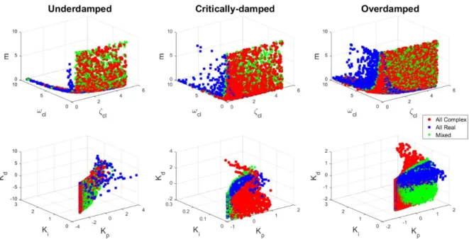
Figure 3: 3D stability region in the design specification and controller parameter space for the three balanced lag-delay processes. (top) design parameter space, (bottom) PID controller parameter space.

Figure 4: 3D stability region in the design specification and controller parameter space for the three delay-dominant processes. (top) design parameter space, (bottom) PID controller parameter space.

It is observed from Figure 2-Figure 4 that the stability regions are wider for high _clwith the two/four complex non-dominant poles, whereas the number of stabilizing data points are only fewer with a demand of high closed loop damping in the case of all real poles. This implies that the centroid of the stabilizing all real non-dominant poles will lie in low closed loop damping region and will yield a less sluggish response than that with the two/four complex non-dominant poles. Also, in the corresponding controller parameter space, the all real non-dominant pole case yields a higher value of Kd.

(17)

Table 1: Number of stable controller gains for the nine test-bench processes using 105_{random Monte Carlo evaluations} Process type Open loop damping Nature of non-dominant pole Alternate stabilizing expressions for Kp Max. no. of stable solutions % Volume s1 _s2 _s3 _s4 Lag dominant Underdamped all complex 503 442 33 1 503 0.503 all real 107 108 32 0 108 0.108

two complex/two real 447 39 47 0 447 0.447

Critically-damped

all complex 1401 264 242 23 1401 1.401

all real 630 330 167 22 630 0.63

Overdamped

all complex 361 292 37 0 361 0.361

all real 62 11 76 0 76 0.076

Balanced lag and delay Underdamped all complex 1028 807 142 22 1028 1.028 all real 376 316 137 15 376 0.376

Critically-damped

all complex 1403 295 237 34 1403 1.403

all real 645 423 161 41 645 0.645

Overdamped

all complex 1356 1146 268 33 1356 1.356

all real 341 32 123 38 341 0.341

Delay dominant

Underdamped

all complex 933 766 114 19 933 0.933

all real 327 199 123 30 327 0.327

Critically-damped

all complex 1007 365 1389 180 1389 1.389

all real 394 0 384 162 394 0.394

Overdamped

all complex 5043 12 2487 349 5043 5.043

all real 2462 568 1057 335 2462 2.462

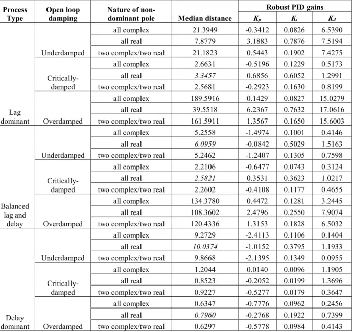
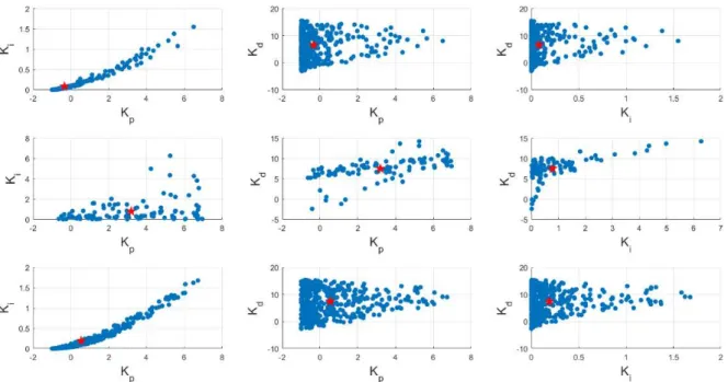
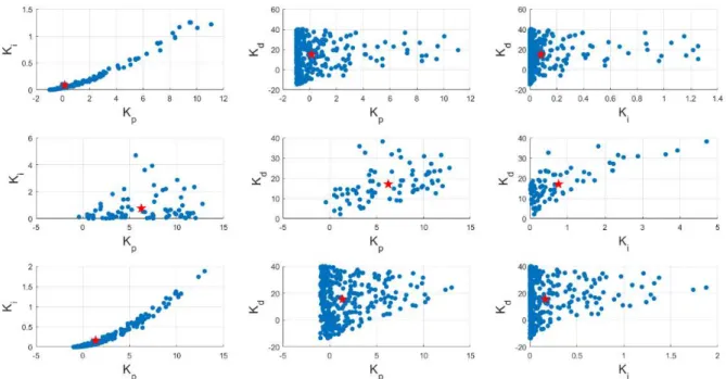
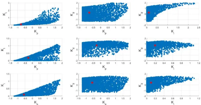
The stabilizing controller gains having the highest percentage volume amongst the four alternative expressions for Kpin Table 1 are now clustered for each type of test-bench process and non-dominant pole types. The centroids of the stability region as identified by 10 independent runs of the k-means clustering algorithm can be considered as the robust stable PID controller gains and are reported in Table 2 for each type of processes and non-dominant pole type. The median distance of all the stabilizing samples from the centroid are also reported in Table 2 indicating compactness of the clusters which is consistently smallest for the all real non-dominant pole type. The projected stability regions in the 2D pair-wise controller parameter space are shown in Figure 5-Figure 13 along with the centroids or the robust stable PID controller gains as the red star, for all the test-bench process types with different lag to delay ratio and open loop oscillation levels. It is evident in most cases that the Kp and Ki (left panels in Figure 5-Figure 13) are more correlated compared to the other pairs of PID controller gains.

We now investigate which cluster has the highest spread in the 3D space of PID controller gains. We also report the median distance between the stabilizing samples and the cluster centroid or the robust stable PID controller gain. The complex shapes of the stabilizing cluster of data-points indicate

(18)

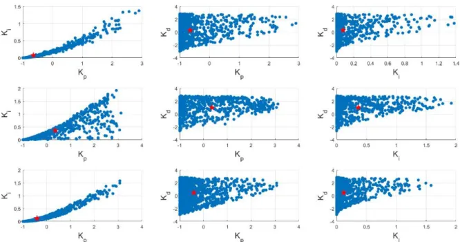
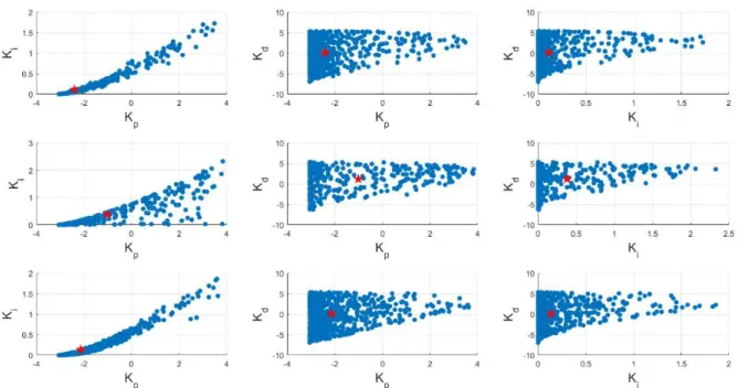
a highly skewed distribution of the stabilizing controller gains as revealed from their histograms in Figure 14. This skewed distribution is a result of different degree of influence of the design parameters or the equivalent controller gains on the shape of the stability regions for each type of test-bench process. This indicates that a different variation of the PID controller gains is possible along different direction or alternatively different extent of parametric uncertainty in the plant model can be allowed using the robust stable solution for the PID controller gains (Silva et al. 2007). Almost in all the cases of the lag-dominant plants, the all real non-dominant poles have the minimum spread (inter-quartile range) and hence the most compact cluster as revealed from the top panel of Figure 14. However for the delay dominant and balanced lag-delay plants the spread become comparable but creates more outliers indicating distant stabilizing regions far away from the centroid which is also evident from the projected 2D scatter diagrams in Figure 8-Figure 13.

Table 2: Robust stable gains and median distance of the stabilizing samples from the centroid Process

Type Open loop damping Nature of non-dominant pole Median distance

Robust PID gains Kp Ki Kd Lag dominant Underdamped all complex 21.3949 -0.3412 0.0826 6.5390 all real 7.8779 3.1883 0.7876 7.5194

two complex/two real 21.1823 0.5443 0.1902 7.4275

Critically-damped

all complex 2.6631 -0.5196 0.1229 0.5173

all real 3.3457 0.6856 0.6052 1.2991

two complex/two real 2.5681 -0.2923 0.1630 0.8199

Overdamped

all complex 189.5916 0.1429 0.0827 15.0279

all real 39.5518 6.2367 0.7632 17.0616

Balanced lag and delay Underdamped all complex 5.2558 -1.4974 0.1001 0.4146 all real 6.0959 -0.0842 0.5029 1.5163

Critically-damped

all complex 2.2106 -0.6477 0.0743 0.3124

all real 2.5821 0.3531 0.3623 1.0217

Overdamped

all complex 134.3780 0.4472 0.1281 3.2445

all real 108.3602 2.4796 0.2550 7.9074

Delay dominant

Underdamped

all complex 9.2729 -2.4113 0.1106 0.1404

all real 10.0374 -1.0152 0.3795 1.1933

Critically-damped

all complex 1.2044 0.0140 0.0096 1.1905

all real 0.8523 -0.2052 0.0199 1.3696

Overdamped

all complex 0.6347 -0.7776 0.0962 0.2456

all real 0.7960 -0.2768 0.1922 0.7399

(19)

Figure 5: Stability regions of PID controller gains to control test-bench plant G1 using different non-dominant pole types as (top) all complex poles, (middle) all real poles, (bottom) two real and two complex poles.

(20)

(21)

(22)

(23)

Figure 14: Distance of the stabilizing samples from the centroid for the nine test-bench processes, indicating compactness of the clusters of data points in the respective stability regions.

4.3. Performance of the robust stable solutions for the test-bench SOPTD processes

In this section, the control performance of the robust stable solutions are quantified for all the nine test-bench processes using the signal norms ( 2 ) or system norms ( 2 ) of different

sensitivity functions, as introduced in section 3.2. The performances are quantified in terms of the disturbance rejection (d), control effort (u), measurement noise filtering (n), tracking error (e), gain margin (Gm), phase margins (_m) and gain cross-over frequency (_gc). Many recent literatures argued that in PID control loops, the disturbance rejection and the control signal affecting the actuator size are considered to be the two most significant criteria (Doyle et al. 2013). However apart from the

(24)

sensitivity function based 2/∞-norms, the traditional performance measures like



Gm,m,gc



are also compared in Table 3 that may help in understanding the robustness to gain variations, oscillations and the speed of the closed loop system respectively, for different robust stable solutions corresponding to the three non-dominant pole types.

Table 3: Control performance with the robust stable PID controller gains for the nine classes of test-bench processes with fixed process parameters

Process type Open loop damping Nature of non-dominant pole

Performance measures of the robust stable PID controller with nominal process parameters

d 2 J _Jd  Ju2 Ju J2n Jn J2e Je Gm m gc Lag dominant Underdamped all complex 3.3044 19.9771 82.7783 4.4093 0.7415 1.0458 3.2822 19.1229 2.3691 57.1641 0.0624 all real 0.4736 1.2697 65.8704 9.4701 1.2351 2.2471 1.3674 2.5484 1.7022 28.6972 0.9056 two complex/ two real 1.4191 6.0633 56.2284 6.6734 0.8891 1.3416 1.6370 5.7103 2.0109 54.0378 0.8813 Critically-damped all complex 3.3439 14.0064 78.7187 1.4461 0.5511 2.0063 3.5184 14.4937 1.6132 38.4221 0.1305 all real 0.8524 2.0666 37.1731 2.3733 0.8002 1.0695 1.1890 2.3550 2.4179 62.6255 0.4096 two complex/ two real 2.3366 8.3256 67.7462 1.2429 0.5160 1.2158 2.5147 8.6536 2.5592 49.7392 0.1481 Overdamped all complex 2.5287 20.5746 76.7873 5.7889 0.4322 1.1142 3.1520 23.3761 2.6707 56.9813 0.0459 all real 0.3742 1.3103 70.3277 13.5142 0.7863 1.7215 1.8449 4.1672 1.8411 37.6897 0.4085 two complex/ two real 1.2487 7.3045 37.4806 7.4410 0.4795 1.0250 2.0481 8.9502 2.4889 90.0900 0.0897 Balanced lag and delay Underdamped all complex 3.6135 17.8317 177.2366 3.5547 0.8981 4.1980 7.2048 35.4755 1.2433 32.0756 0.0740 all real 0.8637 2.3685 78.2454 2.2434 0.5553 1.0199 1.7981 4.6522 3.0004 59.6834 0.2182 two complex/ two real 2.5086 10.3044 137.8486 2.7726 0.6468 2.2735 5.0116 20.4856 1.4595 41.4284 0.0803 Critically-damped all complex 5.0056 24.4705 84.7916 1.5971 0.6311 2.8661 5.1543 24.9874 1.3805 34.1570 0.0926 all real 1.2026 3.2422 41.9556 1.3970 0.6216 1.0275 1.4781 3.4699 2.7956 62.0941 0.2782 two complex/ two real 3.0487 11.6793 63.3211 1.2953 0.4548 1.4710 3.2131 12.0332 1.9285 45.5859 0.1198 Overdamped all complex 1.9220 14.1479 94.6679 1.8423 0.2737 1.6764 3.7439 26.1029 7.9973 34.8646 0.0647 all real 0.8470 4.3265 57.1623 9.4263 0.4782 1.1939 2.2895 9.3214 3.0638 59.7635 0.1123 two complex/ two real 1.2354 7.4122 72.6952 6.0139 0.3896 1.3105 2.7746 14.7869 3.8712 49.1662 0.0813 Delay dominant Underdamped all complex 3.0527 16.3049 271.0282 5.9197 1.0286 5.2373 9.2686 49.4705 1.1931 29.9875 0.0589 all real 0.9421 2.9722 124.1419 3.5254 0.4522 1.1578 2.8602 8.9635 2.1639 53.6541 0.1262 two complex/ two real 2.2789 10.0616 108.0883 4.6069 0.7963 3.2323 6.9138 30.4903 1.3145 37.2722 0.0618 Critically-damped all complex 7.4984 103.7771 64.5575 1.4312 0.7079 1.0000 7.5587 103.7771 2.5635 84.2525 0.0095 all real 6.2557 50.2831 24.6987 1.6705 0.8474 1.0021 6.3342 50.2831 2.0175 64.5762 0.0198 two complex/ two real 8.9267 71.3828 59.5067 1.3151 0.3884 1.8875 8.9794 71.4827 1.5833 43.7891 0.0209 Overdamped all complex 4.0000 19.1321 116.2718 1.9777 0.8174 2.8856 5.0481 23.9850 1.3746 34.3820 0.0965 all real 1.9469 6.5425 59.9512 4.2854 1.5701 1.1506 2.5436 8.2736 1.9999 51.8288 0.1446 two complex/ two real 3.1262 12.5264 77.9316 1.5506 0.9072 1.5167 3.9621 15.6585 1.7872 47.1110 0.0865

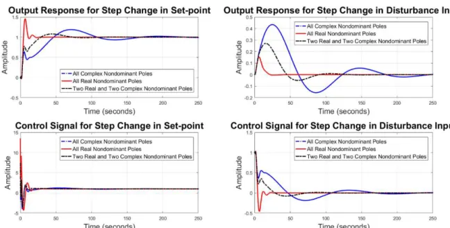
The corresponding time domain responses for control variable due to step change in set-point (left top), step change in disturbance input (right top), manipulated variable or the control signal for step

(25)

change in set-point (left bottom) and control signal for step change in disturbance input (right bottom) are shown in Figure 15-Figure 23, for the nine test-bench processes. Both ₂d

J and d

J are found to be the smallest for the robust stable PID controller with the all real non-dominant pole type, as evident from Table 3 as well as the right top panel of Figure 15-Figure 23.

Figure 15: Controlled variable (top) and manipulated variable (bottom) due to step change in set-point (left) and disturbance input (right) for process G1

The all complex non-dominant pole case has the worst disturbance rejection performance and the two-complex/two-real case falls in between these two cases. The tracking performance is also the best for the all real non-dominant poles as revealed from the values of 2

e

J and_Je

in Table 3 and the responses of the control variables, subjected to a step change in the set-point in the left top panels of Figure 15-Figure 23. For the all complex non-dominant poles, the step response is sluggish and highly oscillatory, amongst the three types of non-dominant poles. However the best tracking and disturbance rejection performance of the all real non-dominant poles comes at the cost of increased

(26)

actuator size (_Ju

) or higher control effort ( 2

u

J ) or both as reported in Table 3 and the two bottom panels of Figure 15-Figure 23, for different test-bench processes. The noise rejection performance is also not always the best using the all real non-dominant poles, as evident from 2

n

J and_Jn

in Table 3. The_gc in Table 3 is always found to be the highest using the all real non-dominant poles, yielding a faster time response. But this increased speed of the robust stable solution comes at the cost of reduced gain and phase margin (Gm,m) in some cases. Therefore, as a summary, control systems where the disturbance rejection, speed of set-point tracking are of utmost importance, the all real dominant pole based robust stable PID controller can be employed. In addition, the all real non-dominant poles also produce the best phase margin particularly for the balanced lag-delay family of processes, as evident from Table 3.

(27)

However some of the above mentioned measures in Table 3, may indicate a similar performance and hence a performance correlation analysis as shown in Figure 24 may reveal which measures are inter-related and which are not. A threshold based analysis of the correlation coefficients (R) of the robust stable performance measures shows that two pairs viz.



J J2d, d



and



J Jd, e



are highly correlated with R>0.9, hence any one of them within the pair would be a sufficiently independent measure of the closed loop performance. This is inherently different from the trade-off based design approach for PID control loops, where it is usually considered that the performance measures are always independent of each other. Therefore, the correlation plots in Figure 24 for the all real non-dominant pole case with best achievable overall performance indicate that improvement in one performance criterion may not always lead to deterioration of the others. In recent years, there have been many works e.g. (Das & Pan 2014)(Herreros et al. 2002; Pan & Das 2012; Pan & Das 2013)(Hajiloo et al. 2012) which have used multi-objective optimization for controller design by

(28)

minimizing multiple conflicting objectives together. However, in most of these cases, the performance correlation analysis was not shown to illustrate whether a chosen set of cost functions or performance measures are at all independent which is an important criterion to judge before designing such optimization-based control systems.

The performance correlation analysis in Figure 24 is particularly important in controller design tasks since there are many recent attempts with an aim of optimization based PID controller tuning using clearly redundant and highly correlated performance measures or cost functions which should have otherwise gone through such performance correlation analysis first, before applying heuristic optimization algorithms on them and comparing marginal performance improvement amongst various competing global optimizers. As prominent examples of such redundant and correlated cost function based PID controller design can be noted in (Panda et al. 2012) and elsewhere. In particular, some

(29)

different ranges which are unjustified e.g. in (Panda et al. 2012). Moreover, for time domain tracking comparisons, usually integral performance indices like integral of absolute error (IAE), integral of squared error (ISE), integral of time multiplied absolute error (ITAE) and integral of time multiplied squared error (ITSE) capture the combined effects of overshoot, steady state error, rise-time, settling-time and peak-settling-time and do not need to be added separately in the cost function unlike the approaches reported in many recent works e.g. (dos Santos Coelho 2009)(Zhu et al. 2009)(Ramezanian et al. 2013)(Sahib 2015)(Bendjeghaba 2014)(Zeng et al. 2015). Therefore including these time domain features either in the cost function along with an integral performance criteria can be considered redundant and unnecessary as previously adopted in (Zamani et al. 2009)(Aguila-Camacho & Duarte-Mermoud 2013) or formulating customized cost functions as weighted average of many correlated cost functions (Das et al. 2011).