Performance Comparison Between Fuzzy Logic Controller (FLC) and PID Controller for a Highly Nonlinear Two-wheels Balancing Robot

Performance Comparison Between Fuzzy Logic Controller (FLC) and PID

Controller for a Highly Nonlinear Two-wheels Balancing Robot

Ahmad Nor Kasruddin Nasir

, Mohd. Ashraf Ahmad

, Riduwan Ghazali

, Nasrul Salim Pakheri

.

Universiti Malaysia Pahang (UMP), 26600 Pekan Pahang.

[email protected], [email protected], [email protected], [email protected].

Abstract—The research on two-wheels balancing robot has gained momentum due to their functionality and reliability when completing certain tasks. This paper presents investigations into the performance comparison of Fuzzy Logic Controller (FLC) and PID controller for a highly nonlinear 2– wheels balancing robot. The mathematical model of 2-wheels balancing robot that is highly nonlinear is derived. The final model suffers from mismatched condition. Two system responses namely the robot position and robot angular position are obtained. The performances of the FLC and PID controllers are examined in terms of input tracking capability. Simulation results of the responses of the nonlinear 2–wheels balancing robot are presented in time domain. A comparative assessment of both control schemes to the system performance is presented and discussed.

Keywords-FLC; PID; Balancing Robot. I. INTRODUCTION (HEADING 1)

The research on two-wheeled balancing robot has gained momentum over the last decade due to the nonlinear and unstable dynamics system. Various control strategies had been proposed by numerous researchers to control the two-wheeled balancing robot such that the robot able to balance itself. In addition, 2-wheels balancing robot is a good platform for researchers to investigate the efficiency of various controllers in control system. Basically, the research on two wheels balancing robot is based on inverted pendulum model. Thus, a two wheels balancing robot needs a good controller to control itself in upright position without the needs from outside.

Motion of two wheels balancing robot is governed by under-actuated configuration, i.e., the number of control

inputs is less than the number of degrees of freedom to be stabilized [1], which makes it difficult to apply the conventional robotics approach for controlling the systems. Due to these reasons, increasing effort has been made towards control designs that guarantee stability and robustness for mobile wheeled inverted pendulums. Although two wheels balancing robot are intrinsically nonlinear and their dynamics will be described by nonlinear differential equations, it is often possible to obtain a linearized model of the system. If the system operates around an operating point, and the signals involved are small signals, a linear model that approximates the nonlinear

system in the region of operation can be obtained. Several techniques for the design of controllers and analysis techniques for linear systems were applied. In [2], motion control was proposed using linear state-space model. In [3], dynamics was derived using a Newtonian approach and the control was design by the equations linearized around an operating point. In [4], the dynamic equations were studied, with the balancing robot pitch and the rotation angles of the two wheels as the variables of interest, and a linear controller was designed for stabilization under the consider of its robustness in [5]. In [6], a linear stabilizing controller was derived by a planar model without considering vehicle yaw. The above control laws are designed on the linearized dynamics which only exhibits desirable behavior around the operating point, and do not have global applicability. In [7], the exact dynamics of two wheels inverted pendulum was investigated, and linear feedback control was developed on the dynamic model. In [8], a two-level velocity controller via partial feedback linearized and a stabilizing position controller were derived; however, the controller design is not robust with respect to parameter uncertainties. In [9], a controller using sliding mode approach was proposed to ensure robustness versus parameter uncertainties for controlling both the position and the orientation of the balancing robot. The mathematical model is established through a modeling process where the system is identified based on the conservation laws and property laws. This process is crucial since a controller is design solely based on this mathematical model. Thus, an accurate equation must be derived in order for the controller to response accordingly.

This paper presents investigations of performance comparison between conventional (PID) and intelligent controller (FLC) schemes for a two wheels balancing robot. The mathematical model of the two wheels balancing robot system is presented in differential equation form with the existence of nonlinear terms. The dynamic model of the system with the permanent magnet DC motors dynamic included is derived based on [10] and [11]. Performances of both control strategy with respect to balancing robot outputs angular position θ and linear position x are examined. Comparative assessment of both control schemes to the two balancing robot system performance is presented and discussed.

2011 First International Conference on Informatics and Computational Intelligence 2011 First International Conference on Informatics and Computational Intelligence

II. DYNAMICSMODEL

Modeling is the process of identifying the principal physical dynamic effects to be considered in analyzing a system, writing the differential and algebraic equations from the conservative laws and property laws of the relevant discipline, and reducing the equations to a convenient differential equation model. This section provides a description on the modeling of the two wheels balancing robot, as a basis of a simulation environment for development and assessment of both control schemes. The robot with its three degrees of freedom is able to linearly move which is characterized by position x, able to rotate around the y-axis (yaw) with associated angle δ and able to

rotate around z-axis (pitch) where the movement is described

by angle θ. List of parameters for the two wheels balancing

robot are shown in Table I. These parameters are based on the project conducted by Ooi (2003) as stated by [11]. The inputs of the system are the voltages VaR and VaL which both are applied to the two motors which located on right side and left side of the robot as shown in Fig. 1. In order to obtain the dynamic model of the balancing robot some assumptions and limitations are introduced;

Motor inductance and friction on the motor armature is neglected.

The wheels of the robot will always stay in contact with the ground.

There is no slip at the wheels. Cornering forces are also negligible.

Fig. 2 shows a free body diagram of the balancing robot which contributed to the nonlinear dynamic equations of the system.

Figure 1. A mobile balancing robot (Grasser et al., 2002)

Figure 2. Free body diagram of balancing robot

Equation (1) represents linear acceleration in x direction, equation (2) represents angular acceleration about y-axis and equation (3) represents angular acceleration about z-axis.

. sin 2 2 cos 2 1 1 1 1 cos 1 cos 1 cos sin 2 2 cos 1 2 l p M dp f l p M drL f drR f aL V l p M r R m k aR V l p M r R m k gl p M x l p M r rR m k e k x (1) . cos sin 2 2 2 1 cos cos cos cos 1 cos 1 sin cos 1 2 l p M dp f p M l drL f l p M drR f l p M aL V r l p M R m k aR V r l p M R m k gl p M x r l p M rR m k e k (2) TABLEI

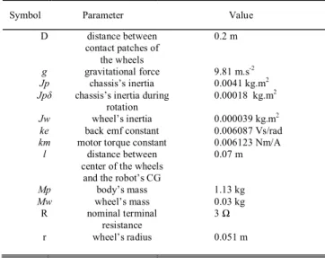
LIST OF PARAMETERS OF TWO-WHEELS BALANCING ROBOT BASED ON [11]

Symbol Parameter Value

D distance between contact patches of the wheels 0.2 m g gravitational force 9.81 m.s-2 Jp chassis’s inertia 0.0041 kg.m2

Jpδ chassis’s inertia during

rotation

0.00018 kg.m2

Jw wheel’s inertia 0.000039 kg.m2

ke back emf constant 0.006087 Vs/rad km motor torque constant 0.006123 Nm/A

l distance between center of the wheels

and the robot’s CG

0.07 m Mp body’s mass 1.13 kg Mw wheel’s mass 0.03 kg R nominal terminal resistance 3 Ω r wheel’s radius 0.051 m

. 2 2 2 2 drL p drR p aL p m aR p m f J D f J D V rR J D k V rR J D k (3)

The symbols of α, β, and γ in equations (1), (2), and (3)

are defined as in equation (4), (5), and (6):

p w w M r J M 2 2₂ (4) 2 2 2_{l cos} M_p (5) 2 l M J_{p p} (6)

As can be seen from equations (1), (2), and (3), all nonlinear terms are remain in the equations. All these equations are used to design the proposed controllers which will be described in the section III.

III. CONTROLLERDESIGN&SIMULATION In this section, two control schemes (FLC and PID) are proposed and described in detail. Furthermore, the following design requirements have been made to examine the performance of both control strategies;

The system overshoot (%OS) of robot position, x is to be at most 10%.

The Rise time (Tr) of robot position, x less than 5 s. The settling time (Ts) of robot position, x and robot

angle θ is to be less than 10 seconds.

Steady-state error is within 2% of the initial value. A. PID Controller

PID stands for Proportional-Integral-Derivative. This is a type of feedback controller whose output, a control variable (CV), is generally based on the error (e) between defined set point (SP) and some measured process variable (PV). Each element of the PID controller refers to a particular action taken on the error. In order to demonstrate the performance of the PID controller in locating the balancing robot to its desired position and angle, the collocated sensor signal of the position of the robot about roll axis, x(s) and angular position of the robot about yaw axis θ(s) are fed back and compared to the reference position, xf(s) and angle θf(s) respectively. Initially, the angular position of the robot which is position about pitch axis is set 0.5 radians. In this study, two PID controllers are required to control the position on the roll axis and the angular position about the yaw axis. The position and angular position errors are regulated through the proportional, integral and derivative gain for each PID controller. Block diagram of the PID controller is shown in Fig. 3, where u1(s) and u2(s) represent the applied voltage at the right motor and left motor respectively. Both of the inputs of the balancing robot are limited to + 20 volts to

Figure 3. Block diagram of PID controller

-20volts. The control signal u1(s) and u2(s) in Fig. 3 can be represented as in equations (7) and (8) respectively

)] ( ) ( ][ [ ) ( 1 1 K 1s r s r s s K K s u I _{D f} P position PID (7) )] ( ) ( ][ [ ) ( 2 ₂ 2 K s s s s K K s u I _{D f} P angle PID (8)

where s is the Laplace variable. Hence the closed-loop transfer function is obtained as in equation (9) and (10).

) ( 1 ) ( ) ( ) ( 1 1 1 1 1 1 s G s K s K K s G s K s K K s r s r I D P I D P f (9) ) ( 1 ) ( ) ( ) ( 2 2 2 2 2 2 s G s K s K K s G s K s K K s s I D P I D P f (10)

In this paper, the Ziegler-Nichols approach is utilized to design both PID controllers. Analyses the tuning process of the proportional, integral and derivative gains using Ziegler-Nichols technique shows that the optimum response of PID controller for controlling linear position is achieved by setting KP1 = -8, KI1 = -0.921 and KD1 = -6, while for controlling angular position, KP2 = -63,KI2 = -60 and KD2 = -11. All the PID1 and PID2 controller parameters must be tuned simultaneously to achieve the best responses as desired.

B. Fuzzy Logic Controller (FLC)

In this part, fuzzy logic controller has been applied for stabilization of the balancing robot as it is a very good choice for control strategy aims because of non-linear and complex mathematical model. The fuzzy logic control (FLC) offers a complete different approach which does not require a precise mathematical modeling of the system nor complex computations in fact it relies on the human

u2(s) u1(s) xf(s) θf(s) θ(s) x(s) _ _ + + PID1 PID2 Nonlinear two wheels balancing robot

Nonlinear Two-Wheeled Balancing Robot Fuzzy Logic Controller 3 Fuzzy Logic Controller 2 Fuzzy Logic Controller 1

+

)

(

t

x

)

(

t

)

(

t

)

(

t

dt

de

e

)

(

t

dt

de

e

)

(

t

x

dt

de

e

)

(

t

u

Figure 4. Block diagram of the system with Fuzzy Logic Controller

capability to understand the systems behavior. Besides, this control technique is based on qualitative control rules. This kind of approach depends on the basic physical properties of the systems, and it is potentially able to extend control capability even to those operating conditions where linear control techniques fail. As a consequence, the application of nonlinear control laws to face the nonlinear nature of balancing robot is easy since fuzzy control is based on heuristic rules. In fact, the FLC approach is general in the sense that almost the same control rules can be applied to a non-linear balancing robot system. It is possible to give two inputs to the FLC as shown in Figure 3. The proposed defuzzification methods for the FLC are sugeno or mamdani. This is because both of these techniques are commonly used in designing the FLC. In order to implement 6 inputs to the controllers, the FLC were divided

into three. As illustrated in Figure 3, the ‘FLC1’controls the

linear position on x-axis, ‘FLC 2’ controls the angular

position y-axis and ‘FLC 3’ controls rotational angle on z-axis of the balancing robot. The ‘FLC 1’ received the

difference (error signal) between position of cart and set point position, x and the rate at which the error of position changes, Δx as the inputs while the ‘FLC 2’ received the

angle error and rate of error of pendulum pole as the inputs

while ‘FLC 3’ received the error and rate of error of rotational angle about z-axis. The control variables of all FLCs were summed together before converted into voltage signal. This signal is then supplied to the dc motors on both left and right sides of the balancing robot.

TABLE II. FUZZY RULE MATRIX FOR CONTROL POSITION FLC

POSITION / ANGLE DELP OS IT ION/ DELANGLE NB NM NS ZE PS PM PB NB NB NM NS NS PS PM PB NM NM NS NS PS PM NS NS NS PS ZE NB NM NS ZE PS PM PB PS NS PS PS PM NM NS PS PS PB NB NM NS PS PS PM

Fig. 5 shows the membership function of FLC’s. The

triangular shape is used to design the FLC.

-3 -2 -1 0 1 2 3 0 0.2 0.4 0.6 0.8 1 Position D egr ee of m em ber shi p NB NM NS ZE PS PM PB

Figure 5. Membership Function of FLC

Table II shows the fuzzy rule matrix for controlling the position and fuzzy rule matrix for controlling the angle respectively. The total rules that should be given are 49 rules. However, there are only 35 rules that are applied to the controllers. In addition, the membership functions were evenly distributed. It is done so that the tuning process of the controller can be easily done. Since the FLC receive six inputs, the difference of the membership function between all the inputs is the range or the universe of discourse. According to the complexity of this balancing robot system, seven fuzzy subsets are needed to quantize each fuzzy variable for three FLCs as shown in Fig. 5. The same quantization has been applied to the all six inputs of the FLC.

IV. RESULTS AND ANALYSIS

In this section, the simulation results of the proposed controller, which is performed on the model of a two wheels balancing robot are presented. Comparative assessment of both control strategies to the system performance are also discussed in details in this section.

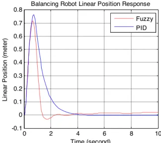
0 2 4 6 8 10 -0.1 0 0.1 0.2 0.3 0.4 0.5 0.6 0.7 0.8 Time (second) Li near P os it ion ( m et er )

Balancing Robot Linear Position Response

Fuzzy PID

Two wheels balancing robot systems with FLC and PID controller block diagram produced two responses, angular position θ and linear position x. As stated earlier, the initial

value of the angular position θ of the balancing robot was set to 0.5 radians. It means that the initial condition of the robot is very unstable. Fig. 6 shows the comparison of the balancing robot linear position response between FLC and PID controller graphically. In this figure, the response for the linear position of the robot with PID controller is represented by straight line or blue color line and the response for the linear position of the robot with FLC controller is represented by dotted line or red color line. Fig. 6 shows that both of the controllers are capable to control the linear position of the nonlinear two wheels balancing robot. Table III shows the summary of the performance characteristics of the balancing robot linear position between FLC and PID controller quantitatively. Based on the data tabulated in Table III, FLC has better settling time of 2.03 seconds while PID has slower settling time of 2.68 seconds. An extra of 0.63 seconds is required for the PID controller balancing robot to balance itself. Similarly, for the maximum overshoot, FLC controller has the best overshoot which is the lowest overshoot between two

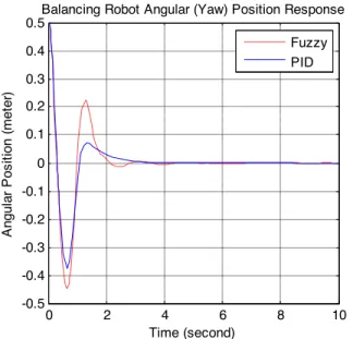
0 2 4 6 8 10 -0.5 -0.4 -0.3 -0.2 -0.1 0 0.1 0.2 0.3 0.4 0.5 Time (second) A ngul ar P os it ion ( m et er )

Balancing Robot Angular (Yaw) Position Response

Fuzzy PID

Figure 7. Two-Wheels Balancing Robot Angular Position Response

controllers. The maximum displacement of the balancing robot when FLC control signal applied to the system is 0.72.meters while maximum displacement of the balancing robot when PID control signal applied to the system is 0.77 meters. A distance of minimum 0.05 meters is required for the PID controller balancing robot to balance itself. Despite the large initial values for the displacement, the proposed FLC controller is able to bring itself to the vertical position. In term of the rise time, balancing robot with PID controller has the fastest rise time 0.37 seconds while balancing robot with FLC controller needs an extra time of 0.03 seconds to rise from 10% to the 90% of the initial value. In term of steady state error, PID controller had shown very outstanding performance by giving zero error at time 6 seconds and more while FLC has 0.02 errors. The responses of the balancing robot linear position have acceptable overshoot and undershoot.

Fig. 7 shows the balancing robot with FLC and PID controller angular position responses. It shows that the result has got similar pattern and not much different. The initial value of the balancing robot angular position is 0.5 radians. The robot needs to balance itself by eliminating the angular position so that the body of the robot remains vertically straight in upright position. Fig. 7 shows that both

0 2 4 6 8 10 -10 -5 0 5 10 15 Time (second) Input V ol tage ( v ol t)

Balancing Robot (left motor) Input Response (volt) Fuzzy PID

Figure 8. Input voltage signal for the left wheel TABLEIII

SUMMARY OF PERFORMANCE CHARACTERISTICS OF THE BALANCING ROBOT LINEAR POSITION BETWEEN FLC AND PID

Time Response

Spesification FLC PID

Rise Time 0.4 sec 0.37sec

Settling Time 2.03 sec 2.68 sec

Steady state error 0.02 0.00

Maximum overshoot 0.72meter 0.77 meter

TABLEIV

SUMMARY OF PERFORMANCE CHARACTERISTICS OF THE BALANCING ROBOT ANGULAR POSITION BETWEEN FLC AND PID

Time Response

Spesification FLC PID

Rise Time 0.37 sec 0.26sec

Settling Time 1.93 sec 2.45 sec

Steady state error 0.00 0.00

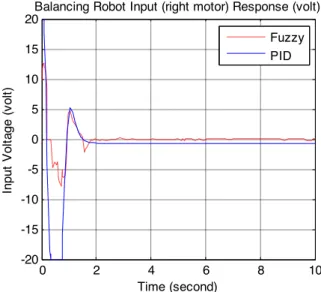
0 2 4 6 8 10 -20 -15 -10 -5 0 5 10 15 20 Time (second) Input V ol tage ( v ol t)

Balancing Robot Input (right motor) Response (volt)

Fuzzy PID

Figure 9. Input voltage signal for the right wheel

of the FLC and PID controllers are capable of controlling the nonlinear unstable balancing robot. Table IV shows the summary of the performance characteristics of the balancing robot angular position between FLC and PID controller quantitatively. Based on the data tabulated in Table IV, FLC has the fastest settling time of 1.93 seconds while PID has the slowest settling time of 2.45 seconds. An extra time of 0.52 seconds is required for the PID controller balancing robot to balance itself. In contrast, for the maximum undershoot, PID controller has the best undershoot which is the lowest undershoot between two controllers. The maximum angular displacement of the balancing robot when FLC control signal applied to the system is -0.45 radians while maximum angular displacement of the balancing robot when PID control signal applied to the system is -0.38 radians. An extra angle of minimum 0.07 meters is required for the FLC controller balancing robot to balance itself. Despite the large initial values for the displacement, the proposed FLC controller is able to bring itself to the vertical position. In term of the rise time, balancing robot with PID controller has the fastest rise time 0.26 seconds while balancing robot with FLC controller needs an extra time of 0.11 seconds to rise from 10% to the 90% of the initial value. In term of steady state error, both of the controllers had shown very outstanding performance by giving zero error at time 4 seconds and more.

The responses of the balancing robot angular position have acceptable overshoot and undershoot. Finally, the input voltages for the left and right wheels are shown in Fig. 8 and Fig. 9 respectively. The input signals for the system were set not to exceed allowable voltage range +20volts to -20 volts.

V. CONCLUSION

In this paper, two controllers such as FLC and PID are successfully designed. Based on the results and the analysis, a conclusion has been made that both of the control method, intelligent controller (FLC) and conventional controller (PID) are capable of controlling the nonlinear two wheels balancing robot angular and linear position. All the successfully designed controllers were compared. The responses of each controller were plotted in one window and are summarized in Table III and Table IV. Simulation results show that FLC controller has better performance compared to PID controller in controlling the nonlinear balancing robot system. It is obviously seen that by applying FLC, input voltage signals for the left and right sides of the wheels did not exceed allowable voltage range. Further improvement need to be done for both of the controllers. PID controller should be improved so that the maximum overshoot for the linear positions do not have very high range as required by the design criteria. On the other side, FLC controller can be

improved so that it’s maximum undershoot and rise time for angular position might be reduced as faster as PID controller.

ACKNOWLEDGMENT

This project has been funded by Universiti Malaysia Pahang, Malaysia.

REFERENCES

[1] A. Isidori, L. Marconi, A. Serrani, Robust Autonomous Guidance: An Internal Model Approach, Springer, New York, 2003..

[2] Y.S. Ha, S. Yuta, Trajectory tracking control for navigation of the inverse pendulum type self-contained mobile robot, Robotics and Autonomous

System 17 (1996) 65–80.

[3] F. Grasser, A. Arrigo, S. Colombi, A.C. Rufer, JOE: a mobile inverted pendulum, IEEE Trans. Indust. Electron. 49 (1) (2002) 107–

114.

[4] A. Salerno, J. Angeles, On the nonlinear controllability of a quasiholonomic mobile robot, in: Proc. IEEE Internat. Conf. on Robotics and Automation, 2003, pp. 3379–3384.

[5] A. Salerno, J. Angeles, The control of semi-autonomous two-wheeled robots undergoing large payload-variations, in: Proc. IEEE Internat. [6] A. Blankespoor, R. Roemer, Experimental verification of the dynamic

model for a quarter size self-balancing wheelchair, in: American Control Conference, 2004, pp. 488–492..

[7] S.S. Ge, C. Wang, Adaptive neural control of uncertain MIMO nonlinear systems, IEEE Trans. Neural Networks 15 (3) (2004) 674–

692.

[8] K. Pathak, J. Franch, S.K. Agrawal, Velocity and position control of a wheeled inverted pendulum by partial feedback linearization, IEEE Trans. Robotics 21 (3) (2005) 505–513.

[9] D.S. Nasrallah, H.Michalska, J. Angeles, Controllability and posture control of a wheeled pendulum moving on an inclined plane, IEEE Trans. Robotics 23 (3) (2007) 564–577.

[10] Grasser, F., D’Arrigo, A., Colombi, S., Rufer, A.C. (2002). JOE: A

Mobile, Inverted Pendulum. IEEE Transactions on Industrial Electronics. 49(1): 107-114.

[11] Ooi, R.C. (2003). Balancing a Two-Wheeled Autonomous Robot. University of Western Australia School of Mechanical Engineering, Australia: B.Sc. Final Year Project.