Neural Network Predicting Remote Vehicle Movement with Vehicle-to-Vehicle Data

(1)

Neural Network Predicting Remote Vehicle Movement with Vehicle-to-Vehicle Data by

Alexander Noel Breg

A thesis submitted in partial fulfillment of the requirements for the degree of

Master of Science in Engineering (Electrical Engineering)

in the University of Michigan-Dearborn 2018

Master’s Thesis Committee:

Professor Yi Lu Murphey, Chair Associate Professor Paul Watta

(2)

(3)

Dedication

This dissertation is dedicated to the memory of Elaine Herzberg, who was the first pedestrian killed by an autonomous vehicle on March 18, 2018.

(4)

Acknowledgements

The research presented in this paper was supported in part by a grant from Mcity and MIDAS at the University of Michigan.

(5)

Table of Contents

Dedication ii

Acknowledgements iii

List of Tables v

List of Figures vi

List of Appendices viii

Abstract ix

Chapter 1 Introduction 1

Chapter 2 Related Technology 4

Chapter 3 System Overview 8

Chapter 4 Experimental Results 20

Chapter 5 Conclusions 30

(6)

List of Tables

Table 1: No median filter truth table ... 22

Table 2: Median 5 filter truth table ... 22

Table 5: 0.2G limit truth table ... 24

Table 8: 1 second prediction neural network truth table... 26

Table 9: 2 second prediction neural network truth table... 26

Table 10: 3 second prediction neural network truth table ... 26

Table 11: 1 second window neural network truth table ... 27

Table 14: 1 second prediction dead reckoning truth table ... 28

Table 15: 2 second prediction dead reckoning truth table ... 28

(7)

List of Figures

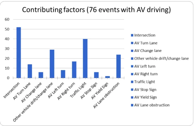
Figure 1: Collision contributing factors to reported autonomous vehicle crashes, State of

California, Department of Motor Vehicles. ... 2

Figure 2: Predictive and classification system schematic ... 9

Figure 3: Example Training Trip ... 11

Figure 4: Example training trip segmentation and normalization ... 12

Figure 5: Neural network layout ... 13

Figure 6: Progression of sliding window of input data to a neural network. ... 14

Figure 7: Remote vehicle unsafe positions ... 14

Figure 8: Initial and final positions of vehicle to determine if host vehicle is sufficiently ahead of remote vehicle to change lanes. ... 15

Figure 9: Neural network prediction categorization ... 19

Figure 10: Neural network relative location prediction and actual... 21

Figure 11: Tenth order filter relative position prediction and actual ... 22

Figure 12: Rationalization of future vehicle position based on kinematics. ... 23

Figure 13: Mean squared error with 5, 10, 15, and 20 hidden layer units ... 25

Figure 14: Mean squared error at 1-3 second prediction ... 25

Figure 15: Mean squared error at 1-3 second window ... 26

Figure 16: Collision factors ... 34

Figure 17: Collision locations ... 35

(8)

Figure 20: Vehicle damage locations ... 36

Figure 21: Vehicle operator ... 37

Figure 22: Situation 1... 38 Figure 23: Situation 2... 39 Figure 24: Situation 3... 39 Figure 25: Situation 4... 40 Figure 26: Situation 5... 40 Figure 27: Situation 6... 41 Figure 28: Situation 7... 41 Figure 29: Situation 8... 42 Figure 30: Situation 9... 42 Figure 31: Situation 10... 43

(9)

List of Appendices

Appendix 1: California Department of Motor Vehicle Autonomous Crash Data ... 34 Appendix 2: Experimental Trips ... 38

(10)

Abstract

This paper presents a neural network developed for predicting the path of a remote vehicle using post facto created vehicle-to-vehicle (V2V) data and uses that prediction to determine whether it is safe for the host vehicle to change lanes. The data was collected in a 2013 experiment involving various drivers traveling on public roads in Ann Arbor, MI. The trips were on suburban roads, city roads and divided highways over a two-day period. The vehicular satellite global positioning system (GPS) data from movement over this period was gathered and post-processed to find vehicle paths within 10 meters of one another. The path traces of the two vehicles were combined to simulate what a V2V network would have provided to properly equipped vehicles if such a network and vehicles existed on real road networks demonstrating natural driving behavior.

This research harnesses this data to determine the increased effectiveness of a neural network predicting the future path of remote vehicles and lane change safety when a V2V network is available. The most studied maneuver is overtaking. To a lesser extent, this paper also provides a view into how a neural network predicts remote vehicle behaviors using a host vehicle equipped with only perceptive hardware and no given information from the remote vehicle.

(11)

Chapter 1 Introduction

Globally, there are 1.25 million deaths related to vehicular transportation every year. [1] In the United States alone in 2015, the National Highway Traffic Safety Administration

(NHTSA) [2] tallied 32,166 traffic deaths and estimated 1,715,000 injuries. Those 6.9 million crashes in 2015 incurred approximately $242 billion in economic costs. The NHTSA survey of the National Motor Vehicle Crash Causation Survey conducted from 2005-2007 (the most recent of this labor intensive and detailed type of study) attributed the critical cause of 94% of accidents to human driver error. [3] In order to improve the safety of vehicular transport, autonomous vehicles are expected to be trained better than humans and correct for most of these human driver errors. And for safety reasons among others, autonomous vehicles have made great strides in commercial investment [4] and technical capability [5]. However, likely due to well publicized accidents including autonomous vehicles, polls in 2018 show a downturn in consumer trust in autonomous vehicles from the prior two years [6]. As consumers recognize the difficulty for a computer to understand and navigate the ambiguous situations of the roads, computer scientists and automotive engineers grapple with the shortcomings of autonomous vehicles. These shortcomings include difficulty in recognizing and giving right of way to human vehicles in merge situations [7], recognizing and avoiding pedestrians and other legged creatures [8], and locating and avoiding stationary objects [9]. So despite how advanced they are currently, autonomous vehicles have weak spots operating in real world scenarios.

(12)

where an autonomous vehicle was controlling the vehicle were a result of the remote, human driven vehicle’s behavior. The collisions are generally minor and occur at estimated speeds of ten miles per hour or less on average. The autonomous vehicle collisions occur at a higher rate than for human drivers [11]. This higher accident rate for computer drivers who perfectly follow the rules of the road indicates that the autonomous vehicle may be obeying the rules, but is still acting differently from what the human drivers are used to and potentially contributing to human driver errors. This increased accident rate demonstrates the continued importance of studying human behavior in vehicles nearby the host vehicle. Figure 1 shows selected contributing factors to the collisions. The figure shows that the collisions involved the autonomous vehicle changing lanes six times and the remote vehicle drifting or changing lanes twenty-nine times. Fifty-two of the seventy-six collisions occurred at an intersection. Appendix 1 contains a complete collection graphs and charts of collision data.

(13)

Continuing to develop an interdisciplinary and multifaceted approach to autonomous vehicle driver systems will be necessary to achieve consumer acceptance of autonomous vehicles. [12] Part of this multidisciplinary approach will be to harness a future vehicle-to-vehicle communication network to enhance situational awareness for all traffic participants. While the primary object avoidance systems for autonomous vehicle are based on LIDAR, cameras, and radar systems, a vehicle-to-vehicle system would add another layer of redundancy and may prove crucial in blind scenarios where line of sight object location is impeded or impossible. Possible impaired scenarios include blind curves, parked vehicles, and buildings encroaching on intersections. Promise of a future vehicle-to-vehicle network is fueled by the increasing prevalence of in-vehicle navigation systems, integrated vehicle modems, and smartphone connectivity. Audi has introduced a vehicle-to-infrastructure system in Las Vegas with certain 2017 model year vehicles. [13] This paper hopes to improve the utilization of vehicle-to-vehicle data when it becomes available in the near future.

(14)

Chapter 2 Related Technology

Hidden Markov Models (HMM) have been a common and useful path prediction technique. Streubel and Hoffmann [14] used an HMM to predict driver intent at a four way intersection. HMM is a stochastic model which describes a dynamic process through two random processes (Markov Chains). One process is hidden and represents the state transition of the system. The other process produces observations during each step. The Markov attribute represents the uncertainty of the process. The system contains a defined number of degrees of freedom. Model parameters must be determined. The system needs to learn the optimal model parameters that maximizes the probability for existing observation sequences. The system also needs to learn the representation or probability for an existing observation sequence being created by the HMM. The latter is solvable by a forward algorithm. Learning has no known algorithm and is found by an Expectation-Maximization-algorithm.

Sreubal and Hoffman analyzed intersection approaches from 100 meters away from the center of the intersection to the center of the intersection. GPS data was used to determine position. The data features were velocity, acceleration, yaw rate, and distance to intersection. They clustered the data based on a Gaussian mixture approach and a k-means clustering. There was high variation in the straight data because of the sheer number of data points and

comparatively less variation with turning left because there were less data points. The HMM model recognized turning left and right sequences better because of the low fluctuation between the sequences. The acceleration in some sequences deviates strongly from zero. Variations in the HMM used are number of hidden states, symbols and sequences. Left turning sequences 100%

(15)

had a 100 percent correct prediction rate. All types of turning prediction had a correct prediction rate of 68-82 percent. For all types of sequences, they claim 90 percent prediction rate up to seven seconds in advance. Mean prediction times were 8.3, 4.7, and 8.3 for left, right, and straight respectively.

Hubmann et al. [15] use a partially observable Markov decision process (POMDP) to continuously manage the longitudinal speed of a simulated vehicle through a simulated

intersection. The process is able to update every second to safely and interactively navigate the vehicle through an intersection by incorporating more information as the situation evolves. The process examines many possible trajectories of the vehicles involved and intelligently expands upon the most promising possibilities.

The technique hopes to account for the uncertainties of other road users’ trajectories including: the unknown intention of other drivers, their future travel, the effects of the host vehicle on their routes, and the noise of sensors and the interpretation of the sensors. The technique assumes that information about the situation will improve over time and incorporates this improved information in the host vehicle path planning. To simplify their path planning, they assume a pre-planned trajectory and only control the longitudinal velocity.

Wen, Zhang, et al. [16] found that for lane change maneuvers Hidden Conditional Random Fields (HCRF) improved prediction of driver intent versus HMM and support vector machines (SVM). The input features are steering wheel angle, lateral position, and driver’s gaze. HCRF is an undirected graph useful for sequence labeling. HCRF assumes that there is a hidden label associated with each labeled sequence. Each label is given a probability function given a sequence. A potential function describes the relationship between the hidden variable and the sequence label. For training, marginal probabilities of hidden variables calculate gradients.

(16)

Recurrent neural networks (RNNs) are a more recent phenomenon to predict the paths of vehicles. As Zyner, Worrall, et al. show in [17], Long Term Short Term RNNs hold promise for predicting future vehicle trajectories especially through the finite number of trajectories of an intersection. RNNs are most effective with order dependent data, such as position versus time data of vehicle tracks. Using a many into one type of RNN, the paper uses entire segments of Kalman filter fused vehicle speed, inertia, and position relative to the intersection using

odometry and a GPS. The use of a Long Term Short Term memory allows the retention of data for an arbitrary length of time. The Long Short Term Memory variation allows the model to consider short periods of time instead of a single time step of data. Further, using maneuver based modeling, which assumes that a finite number of moves can be executed through the intersection, the paper shows a variety of ability to predict the subject vehicle’s path through the intersection from three different approaches to a T-junction intersection.

For vehicle path detection within the context of intelligent vehicles, computer vision based technologies have been explored extensively. Deo, Rangsh, and Trivedi [18] show real time processing of remote vehicles can be achieved using a mobile computer. Their system processed data from eight cameras on a California highway at six frames per second, which they claim is sufficient for real world applications. The system consists of a hidden Markov model based maneuver recognition model, a trajectory prediction module based on the amalgamation of interacting multiple model and maneuver specific variational Gaussian mixture models, and a vehicle interaction module that considers the global context of remote vehicles and assigns final predictions by minimizing an energy function based on the outputs of the other modules.

This dissertation bases its approach and analysis primarily on a Murphey, et al. paper [19]. That paper shows improvement in the prediction of the path of a pedestrian carrying GPS

(17)

with a trained neural network compared to constant velocity and constant acceleration

approaches, particularly at longer prediction times (greater than one second). The goal of the neural network was to provide a host vehicle with the future location of a pedestrian in sufficient time to avoid a collision. Predicting the position of a remote person or object at a predictive length greater than one second is useful for helping a host vehicle gain confidence in its navigation ability and should help the adoption of autonomous vehicles.

(18)

Chapter 3 System Overview

A.Purpose

This paper offers a unique approach by mining human driver data recorded on real roads with natural driving behavior. It uses the present and past positions of the two vehicles to determine the future relative position of the remote vehicle relative to the host vehicle and predicts whether or not it is safe for the host vehicle to change lanes given the future remote vehicle relative position. The total system can be thought of as an enhanced version of the currently available blind spot warning systems with the ability to predict whether the remote vehicle will be in the path of the host vehicle instead of only informing the driver whether or not the remote vehicle is at present in an unsafe relative position.

B. Components

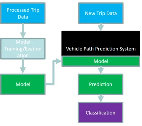
The system consists of two main components, the path predicting neural network and the lane change “safe” or “unsafe” classification system. Figure 2 provides a schematic of the system flow. The left column shows the path predicting neural network training and the right column shows the path prediction of each vehicle’s future path, determination of a relative location, and classification that relative location as “safe” or “unsafe” for the host vehicle to change lanes.

(19)

Figure 2: Predictive and classification system schematic

The path predicting neural network was trained with varying windows sizes, predictive lengths, filters, features, and hidden units on a set of vehicle trips. After training on a set of 100 vehicle tracks, the path prediction neural network was applied to an exclusive and distinct set of ten situations where two vehicles were recorded traveling within ten meters of one another. The effectiveness of the path predicting neural network is assessed with a four-fold cross-validated mean squared error of position.

After receiving predicted and actual positions, the classification system first changes both the predicted and actual GPS location of the remote and host vehicles position into relative position, velocity, and direction to a domain based on the host vehicle. Then the classification system classifies the predicted and actual relative GPS positions in the data sets as “safe” or “unsafe.” Once the predicted relative position of the remote vehicle is classified as “safe” and

(20)

“unsafe,” the predicted relative position set of classifications is compared to the actual relative GPS position set of classifications at each time stamp. The performance of the classification portion of the system is assessed by truth table. A dead reckoning path prediction system based on the relative position and velocity of the remote vehicle to the host vehicle was added to the classification system to provide a relative measure of classification success.

C.Data Sets

In order to study vehicle-to-vehicle behavior, a 5,873 trip dataset of vehicles traveling in the Ann Arbor, Michigan area is used as a repository from which to select interesting data sets. From this data set two groups of trips are selected. Both sets of data consist of trips with high confidence of GPS signal accuracy. The first data set is used to train the neural network to predict the future position of any vehicle from the data set. From the large set of trips with a high confidence GPS location, a smaller set of data is created to make an ad-hoc data set of vehicle-to-vehicle interactions in a post facto vehicle-to-vehicle network. Using a Matlab tool, the locations in the dataset are compared to one another to find trips that interact within a ten meters of another vehicle. Then the trips which pass within ten meters of each other are clipped to the period of time during which they are within thirty meters of each other to provide a focused set of data. Given the prevalence of autonomous vehicle accidents at intersections and during lane changes, this paper will select from the metadata set 10 examples of vehicle

interaction within ten meters near intersections and with lane changes.

After selection, the trip data was broken into segments to fill the sample window for each predictive time step. Each segment’s location data was normalized to the first data sample in the segment. That is, the first sample is considered the origin of all subsequent location data for the segment. In order to provide coordinates which could be converted into normalized

(21)

segments, the data was converted from degrees of latitude and longitude into the Universal Transverse Mercator (UTM) coordinate system via Matlab program by F. Beauducel. The UTM coordinate system represents the Earth in a 60 zone grid. Each zone covers 6° of longitude and ranges from 80°S to 84°N latitude. The UTM coordinates of a point at time are denoted as

and . In order to make the path segments insensitive to the trip starting point, the system uses the initial segment point and a scaling factor. Therefore,

and

where .

(22)

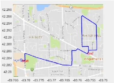
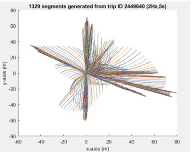
Figure 3 shows an example of a training trip and figure 4 shows what the each segment input into the neural network looks like after each segment has been normalized to a common origin.

Figure 4: Example training trip segmentation and normalization

D.Data Source

Data was collected by volunteer drivers over a two day period in 2013. The vehicle GPS location at a rate of 10 Hz was then analyzed for trip sequences in which one vehicle came within ten meters of another vehicle to create post facto vehicle-to-vehicle network. From the data set, 100 trips were chosen of individual vehicle paths on Ann Arbor roads for training the neural network with the following filtering criteria:

● Maximum velocity of 21 m/s

● Trip duration between 600 and 900 seconds

● Distance traveled between 4 and 15 km

● District name (Google geo address api) Ann Arbor

In order to remove the noise prevalent in raw GPS location data, the raw data was processed by applying median and mean filters in order to smooth the data before being used to train the neural network. GPS speed and heading from the vehicles was extracted from the

(23)

filtered position data was therefore input into the neural network unfiltered after the positions were already filtered.

E. Predictive method

The future positions of the host and remote vehicles were independently predicted by a neural network, and its performance was compared to a dead reckoning system. The Matlab neural network tool trained the multilayer perceptron neural networks and test their efficacy with 5, 10, 15, or 20 hidden units and 2 output layers. The hidden units feature tan-sigmoid transfer functions and the two output layers of each network use a linear transfer function. The training was conducted with the Levenberg-Marquardt training technique with four-fold cross-validation. The performance was assessed with mean squared error of location in meters. A layout of the fifteen hidden unit neural network is shown in figure 5 with a two-second window of four features of ten Hertz data.

Figure 5: Neural network layout

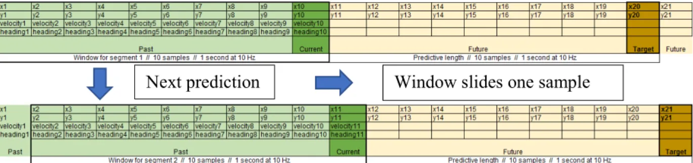
The neural network was trained with a variety of settings including varied window size, predictive length, and number of hidden units. Figure 6 shows a diagram of the progression of a sliding ten event window across the four feature matrix of the vehicle position and velocity at each sample. The transverse (x-position) and longitudinal (y-position) of the vehicle positions are derived from the recorded GPS positions of the two vehicles. The velocity of the two

(24)

vehicles and headings are extracted features from the GPS position data.

Figure 6: Progression of sliding window of input data to a neural network.

F. Design of Experiment

In order to provide a challenging test environment for the classification portion of the system, short segments of up to 30 seconds with portions with a vehicle nearby were cut from the meta-dataset with no overlap between the training set and the test set. Segments were chosen due to the presence of a vehicle-overtaking maneuver, preferably with at an intersection. The segments featured a mix of samples with the remote vehicle in a position safe and unsafe for a host vehicle lane-change maneuver.

Figure 7: Remote vehicle unsafe positions

Figure 7 shows the relative remote vehicle position classification zone diagram. The “Speed Dependent Cushion” is defined in the next section based on an assumed acceleration rate

(25)

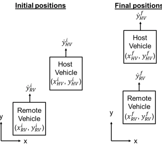
of the host vehicle and the speed at which the remote vehicle is approaching the host vehicle to allow sufficient time for the host vehicle to maneuver in front of the remote vehicle and maintain a safe distance in front of the remote vehicle. Figure 8 illustrates the initial and final host and remote vehicle positions in order to define the variables used in the equations below.

Figure 8: Initial and final positions of vehicle to determine if host vehicle is sufficiently ahead of remote vehicle to change lanes.

The speed dependent cushion is determined by solving two kinematic equations. The first is based on the assumed average acceleration of the host, which is 2 m/s2_{in this case based}

on a conservative rate of acceleration. Given that in order to execute a lane change without impeding the vehicle approaching from the rear, the final velocity of both vehicles will be the same.

(26)

(1)

(2)

(3) After solving for the time to accelerate up to the remote vehicle’s constant velocity, the kinematic equation describing the future position of both vehicles yields equations four and five.

(4)

(5) Subtracting equation five from equation four and assuming that the remote vehicle has no acceleration yields equation six.

(6) It is desired that the relative positions of the two vehicles provides space for half the length l of each vehicle assuming that the GPS location is at the geometric center of the two vehicles and that there is a safety cushion of three seconds between them, so the final relative position should be as shown in equation seven.

(27)

+ ₍₇₎

Substituting the right hand side of equation seven for the left hand side of equation six gives equation eight.

(8) This yields that the relative initial position of the two vehicles must be as described in equation nine in order to have a safe final distance between them.

(9) The other variable which changes in equation nine is the time cushion based on the predictive length being used. If the predictive length is longer, then the host vehicle needs less cushion to execute the maneuver because the predicted location is taking into consideration the future location of the remote vehicle. The time cushion is three seconds less the predictive length of the predictive method to account for the fact that the prediction will account for the other vehicle’s future position.

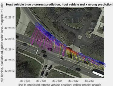
A Matlab program categorized the predicted results as “safe” and “unsafe” and compared them to the known future vehicle positions categorization as “safe” or “unsafe.” An example of the graphical output of the system is shown in figure 9 with a full set of images available upon request. The ‘x’s and ‘o’s show the host vehicle traveling onto and on ramp while the remote vehicle passes one and then two lanes to the driver’s side of the host vehicle. ‘x’ signifies an

(28)

versus the actual GPS position. The lines emanating from the host vehicle’s ‘x’s and ‘o’s show the direction and distance of the remote vehicle relative to the host vehicle. The color of the lines emanating from the host vehicle to the predicted remote vehicle position indicate the predicted position classification. Yellow lines indicate that the remote vehicle was in the “unsafe” zone for the host vehicle to change lanes. Red lines (not shown) indicate that the remote vehicles predicted position was behind the “unsafe” zone. Blue lines (not shown) indicate that the remote vehicle was ahead of the unsafe zone. The magenta lines indicate that the remote vehicle’s predicted position was more than one lane away from the host vehicle. Finally, a green line indicates that the remote vehicle’s predicted position is in the same lane as the host vehicle.

Figure 9 shows how precise the future vehicle position must be to have a consistently correct classification of the remote vehicle’s future position. The “unsafe” prediction is very difficult to earn a high classification accuracy on because of how few “unsafe” data samples there were and how small deviation from the noisy GPS “truth” values the prediction values can lead to misclassification. Figure 9 also gives a good idea of how difficult and subtle the

situations examined are. In figure 9, the host vehicle makes a slight maneuver to its passenger side, which gradually increases the lateral distance to the passing remote vehicle such that the remote vehicle no longer is within the “unsafe” zone of the host vehicle.

(29)

(30)

Chapter 4 Experimental Results

This section compares many different approaches to improving the predicted relative position of the remote vehicle to the host vehicle with a neural network. The experimentation included comparing the four-fold cross validation mean squared error of various window sizes, predictive lengths, features, and hidden units in the single hidden layer. The outputted predicted position was smoothed by both a median filter and in an unsuccessful attempt, clipped by a kinematic rationalization of the future remote vehicles position based on extracted relative velocity and different acceleration limits. The effect of these changes was measured both by a comparison of the mean squared error of the predicted position and a comparison of the truth tables for the classification of the predicted relative position of the remote vehicle to the host vehicle.

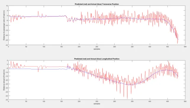
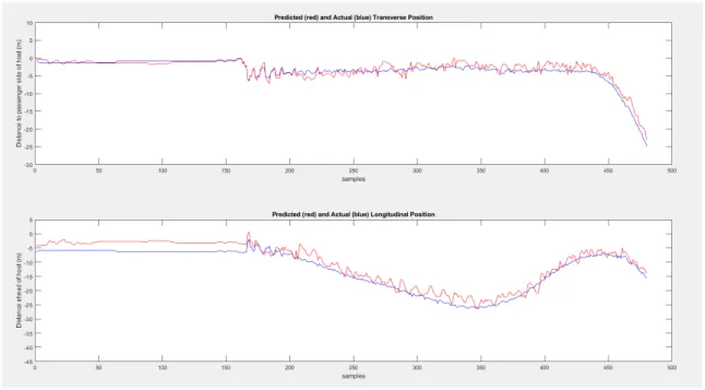
As figure 10 shows, the output of a neural network location prediction system is noisy compared to the actual GPS tracked position of the remote vehicle relative to the host vehicle.

(31)

Figure 10: Neural network relative location prediction and actual

A variety of median filters was applied to the output. The median filters had the following equations where n is the order of the filter and k is the time stamp of the data:

● When n is odd, y(k) is the median of

.

● When n is even, y(k) is the median of

In case that n is even, medfilt1 sorts the numbers and takes the average of the two middle elements of the sorted list.

Figure 11 shows the improvement that the tenth order median filter made on a sample of predicted position from the output of the neural network in red versus the blue mean and median filtered actual GPS position compared to the unfiltered predicted position shown in figure 10.

(32)

Figure 11: Tenth order filter relative position prediction and actual No Median Filter Truth Table

Actual Predicted Safe Unsafe Safe 0.8452 0.1548 Unsafe 0.3905 0.6095 Table 1: No median filter truth table

Median 5 Filter Truth Table Actual Predicted Safe Unsafe Safe 0.8452 0.1548

Unsafe 0.2 0.8

Table 2: Median 5 filter truth table Median 10 Filter Truth Table Actual Predicted Safe Unsafe Safe 0.8579 0.1421 Unsafe 0.0857 0.9143 Table 3: Median 10 filter truth table

Median 20 Filter Truth Table Actual Predicted Safe Unsafe Safe 0.8706 0.1294 Unsafe 0.0952 0.9048 Table 4: Median 20 filter truth table

(33)

Comparing tables one through four, the tenth order median filter offered the best overall results with over 80 percent correct classification of both the “safe” and “unsafe” situations. The twentieth order median filter had similar results to the tenth order filter, but to be conservative, the less filtered data is preferred.

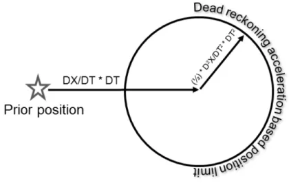
Another process to smooth the output of the neural network data is a rationalization process derived from the physical realities governing the kinematics of vehicle dynamics. The output of the neural network was limited to an area defined by a dead reckoning calculation of the next vehicle location expanded by a ring determined by maximum acceleration limited by tire grip. Most non-sports cars in automotive skid pad testing exhibit grip less than 9.8 m/s^2. Most non-emergency vehicle acceleration is less than 4 m/s^2. As the limit for acceleration decreases, the prediction becomes smoother, more similar to a dead-reckoning approach, and

non-conservative due to expecting only a limited amount of acceleration. Results from limitations on the location of neural network predictions are in tables 5-7 with limits of acceleration ranging from 0.2 to 0.6 times the acceleration due to gravity on Earth’s surface.

(34)

0.2 G Limit Truth Table Percent Actual Predicted Safe Unsafe Safe 0.8452 0.1548 Unsafe 0.3905 0.6095 Table 5: 0.2G limit truth table

Changing the limit of acceleration had no effect on the classification of “safe” and “unsafe” maneuvers versus the no filter results shown in table 1. The predicted position results from the kinematic limited method were discarded because the method had no advantage over the median filter and adds complexity.

Figure 13 shows that the number of hidden layer units did not improve the mean squared error of the location prediction significantly or consistently beyond ten hidden layers. Therefore, to improve simplicity, the experimentation with prediction lengths and window sizes will occur with ten hidden units in the neural network.

(35)

Figure 13: Mean squared error with 5, 10, 15, and 20 hidden layer units

Figure 14 shows that the mean squared error of the position increases with predictive time.

Figure 14: Mean squared error at 1-3 second prediction

Figure 15 shows that changing the window does not have a significant effect on the predictive ability of the neural network. The twenty sample window size has the lowest peak of mean squared error and will be used for the other neural network classification attempts.

(36)

Figure 15: Mean squared error at 1-3 second window

The experimentation between predictive lengths and window sizes was conducted with a tenth order median filter. The predictive length classifications with varying predictive lengths have ten hidden units and two second windows.

1 second prediction Truth Table Actual Predicted Safe Unsafe

Safe 0.97 0.3

Unsafe 0.0036 0.9964 Table 8: 1 second prediction neural network truth table

2 second prediction Truth Table Actual Predicted Safe Unsafe Safe 0.8579 0.1421 Unsafe 0.0857 0.9143 Table 9: 2 second prediction neural network truth table

3 second prediction Truth Table Actual Predicted Safe Unsafe Safe 0.9397 0.0603 Unsafe 0.375 0.625

(37)

Tables 8 -10 show the prediction classification rate for various predictive lengths. The correct classification rate was very high and near perfect for the one second predictive length. Accuracy decreased at the longer predictive lengths but the two second predictive length had eighty-six and ninety-one percent accuracy for the “safe” and “unsafe” categorizations, respectively. The three second predictive length had a big reduction in “unsafe” prediction classification rate, and this may be due to a bias towards predicting safe as the “safe” classification rate increased for both the “safe” and “unsafe” actual data samples.

The next experiment compared window sizes from one to three seconds. Every neural network had a two second predictive length and ten hidden units. The position output of the neural network was filtered with a tenth order filter.

1 second window Truth Table Actual Predicted Safe Unsafe Safe 0.9752 0.0248 Unsafe 0.6952 0.3048 Table 11: 1 second window neural network truth table

Table 11 shows that the one second window is perhaps too short as it has poor prediction of the “unsafe” cases. Comparing tables 12 and 13 shows the two second window to be

(38)

preferable because it requires less data and has a more conservative prediction with fourteen percentage point advantage in “unsafe” classification rate.

1 second DR Truth Table Actual Predicted Safe Unsafe Safe 0.9835 0.0165 Unsafe 0.0145 0.9855

Table 14: 1 second prediction dead reckoning truth table 2 second DR Truth Table

Actual Predicted Safe Unsafe Safe 0.8094 0.1906 Unsafe 0.5619 0.4381

Table 15: 2 second prediction dead reckoning truth table 3 second DR Truth Table

Actual Predicted Safe Unsafe Safe 0.9267 0.0733

Unsafe 1 0

Table 16: 3 second prediction dead reckoning truth table

The dead reckoning results were similar to the neural network results at times, however there were some significant gains for the neural network correct classification rate. Comparing tables 14 for the dead reckoning approach and table 8 for the neural network path prediction approach shows a very similar and high prediction rates for both the dead reckoning approach and the neural network approach at the one second predictive length. The results are more divergent when comparing table fifteen for the dead reckoning approach and table nine for the neural network approach. The two approaches were within five percentage points correct classification for the “safe” condition, but the neural network had a forty-seven percentage point advantage for the unsafe classification. The stark advantage on the “unsafe” classification may be due to the small number of instances of “unsafe” instances versus “safe” instances. Finally, the three second prediction length shows a similar advantage for the neural network approach

(39)

over the dead reckoning approach with nearly the same “safe” correct classification rate but a sixty-three percentage point advantage for the neural network approach for the classification of “unsafe” situations. Overall, the neural network is the same or significantly better than the dead reckoning approach to classifying the future relative position of the remote vehicle as “safe” or “unsafe” at varying predictive lengths, which are advantageous to the current blind spot warning systems on automobiles.

(40)

Chapter 5 Conclusions

Accurate, timely, and robust prediction of the path of remote vehicles is critical for the safe travel of an autonomous vehicle. For the foreseeable future, remote vehicles will

predominantly be human driven. Bansal and Kockelman [20] expect between twenty-five to eighty-seven percent prevalence of autonomous vehicles in the U.S. vehicle fleet by 2045. Based on deployment and adoption of previous vehicle technologies (like automatic transmission, airbags, vehicle navigation systems, and hybrid-electric drive), Litman [21]

forecasts that AVs will constitute around 50% of vehicle fleet, 90% of vehicle sales, and 65% of all vehicle travel by 2050. Both estimates show that well into the future there will be a mix of autonomous and human driven vehicles on the road.

Sharing the roadways with fellow human drivers means that the traffic around

autonomous vehicles will be unpredictable when humans fail to obey the rules of the road or fail to maintain control of their vehicle. As autonomous vehicles driving on California roads have found out, remote vehicles driven by humans are the predominant cause of autonomous vehicle collisions. In seventy-three of seventy-six traffic collisions reported to the State of California Department of Motor Vehicles, [10] the remote human driven vehicle was the cause of the collision. In such an uncertain environment, the virtual driver system of the autonomous vehicle must possess strong, robust predictive abilities in order to help the autonomous vehicle avoid collisions, even if the other driver would have been at fault had the collision occurred.

Strong predictive ability will improve adoption and acceptance of autonomous vehicles. A 2017 Gartner survey [22] reveals that fifty-five percent of 1519 respondents in the United

(41)

States and Germany will not ride in a fully autonomous vehicle. Autonomous vehicles will be deployed to a skeptical audience, so as seamless as possible a deployment will be key to their adoption. Specifically, “fear of autonomous vehicles getting confused by unexpected situations” was a concern of respondents. Improving all types of autonomous accident avoidance, including for situations where the accident is caused not by the inability of the autonomous vehicle to follow the rules of the road, will increase autonomous vehicle adoption.

The neural network approach to predicting whether the remote vehicle will be in an unsafe position for the host vehicle to make a lane change maneuver improved the classification rate as recorded by the truth tables by one to sixty-three percentage points. This advantage for the neural network was achieved with ten hidden nodes in the single hidden layer within the network, a two-second window, four feature vectors, and with a median filter smoothing the predicted position of the remote vehicle’s relative position to the host vehicle.

This paper provides a unique perspective on the prediction of remote vehicle behavior because it analyzes data created by nearly unsuspecting remote vehicles and simulates a future traffic scheme with vehicles communicating with a vehicle-to-vehicle network.

The results of this paper compare various neural network characteristics to predict remote vehicle behavior. Future improvements will include harnessing recurrent neural networks, which stress the most recent data in the predictive data set. Also, maneuver recognition may be possible if there are sufficient examples of a maneuver type. However, there were only a few examples of each maneuver type collected over two days of vehicles driving examined in this study, so more data will need to be collected to accomplish maneuver recognition.

The GPS data has not only noise but discontinuities as well. The discontinuities are caused by drops in the GPS signal caused by hardware deficiencies and obstacles such as bridges

(42)

and buildings. Park, Lee, and Seo [23] found that the accuracy and availability of the position, navigation, and timing information from a global navigation satellite system can be interfered with by the ionosphere, multipath signals, and radio frequency interference (RFI). The discontinuities were eliminated from the data sets in this experiment manually in order to simplify the analysis and make the prediction results more consistent between runs with and without interruptions in the data. The interruptions in the signal caused the predictions of next vehicle position to be wildly inaccurate. However, this simplification is not as easy to

implement in a real car. A signal quality metric will be needed to determine the validity of the GPS data or the quality of the transmitted vehicle-to-vehicle transmitted network position. Perhaps, the position data will be augmented by more reliable locally derived position, direction, and vehicle speed measurements fed into a Kalman filter. The difficulty of maintaining a

continuous stream of data for the system both from the initial determination of remote vehicle location and the transmission of the data is an important area of consideration.

Furthermore regarding remote vehicle data collection and transmission, future study regarding vehicle-to-vehicle communication should include consideration for the time to collect, communicate, and process the data necessary to make future vehicle position predictions. This study assumes that the collection, transmission, and processing of data occurs instantly. The simplification helps to compensate for the lack of readily available and useful car area network (CAN) signals. Ideally, the data passed from one vehicle to another should include accelerator and brake pedal positions and steering wheel angle to help predict future positions. The addition of these basic vehicle signals would greatly improve the certainty of the remote vehicle position by the implementation of a more sophisticated Kalman filter than this paper features by including these highly predictive signals to vehicle movement.

(43)

Another limitation of this paper is that the data collected for this experiment contain no crashes, which is an important set of data to analyze for system robustness. Data with crashes within it are not totally necessary given that the real world implementation of this system would be to create an enhanced blind spot monitoring system. Simply having situations where the host vehicle would have crashed if it changed lanes and cases where it would not have if the host vehicle were to change lanes into it is sufficient to show the range of situations. However, a future study which contains data where the host vehicle crashes into the remote vehicle either by sheer volume of trip collection or some kind of simulation would be helpful to rigorously test the system and show the helpfulness of the system.

(44)

Appendix 1: California Department of Motor Vehicle Autonomous Crash Data

(45)

Figure 17: Collision locations

(46)

Figure 19: Collision speeds

(47)

(48)

Appendix 2: Experimental Trips

Pink – host vehicle, correct remote position prediction Red – host vehicle, incorrect remote position prediction Blue – true remote vehicle position

White – predicted remote vehicle position

Green – line connecting host and predicted remote vehicle prediction

(49)

Figure 23: Situation 2

(50)

(51)

(52)

(53)

(54)

Bibliography

[1] World Health Organization, Road Traffic Injuries Fact Sheet, May 2017, http://www.who.int/mediacentre/factsheets/fs358/en/, Web, November 19, 2018.

[2] National Highway Traffic Safety Administration, “Summary of Motor Vehicle Crashes” (Final Edition), Traffic Safety Facts, 2015 Data, October 2017.

https://crashstats.nhtsa.dot.gov/Api/Public/ViewPublication/812376, Web, November 19, 2018. [3] National Highway Traffic Safety Administration, “Critical Reasons for Crashes

Investigated in the National Motor Vehicle Crash Causation Survey,” Traffic Safety Facts, February 2015, https://crashstats.nhtsa.dot.gov/Api/Public/ViewPublication/812115, Web, November 19, 2018.

[4] “Autonomy is Driving a Surge of Auto Tech Investment,” CB Insights, September 27, 2018, https://www.cbinsights.com/research/auto-tech-startup-investment-trends/, Web, November 18, 2018.

[5] J. Yu and L. Petnga, “Space-based Collision Avoidance Framework for Autonomous Vehicles,” Procedia Computer Science, Vol. 140, 2018, p. 37-45.

[6] “Autonomous Vehicle Awareness Rising, Acceptance Declining, According to Cox Automotive Mobility Study,” Cox Automotive, Aug 16, 2018,

https://www.prnewswire.com/news-releases/autonomous-vehicle-awareness-rising-acceptance-declining-according-to-cox-automotive-mobility-study-300697862.html, Web, November 18, 2018.

[7] C. Urmson (2016), “Report of traffic accident involving an autonomous vehicle”, State of California Department of Motor Vehicle.

[8] A. Marshall (2018), “The Uber crash won’t be the last shocking self-driving death”, Transportation, Wired,

https://www.wired.com/story/uber-self-driving-crash-explanation-lidar-sensors/, Web, November, 18 2018.

[9] J. Stewart (2018), “Why Tesla’s autopilot can’t see a stopped firetruck?”, Transportation,

(55)

[10] “Report of Traffic Collision Involving an Autonomous Vehicle, (OL 316), State of California, Department of Motor Vehicles,

https://www.dmv.ca.gov/portal/dmv/detail/vr/autonomous/autonomousveh_ol316+, Web, November 18, 2018.

[11] F. Favarò, S. Eurich, and N. Nader, “Autonomous vehicles’ disengagements: Trends, triggers, and regulatory Limitations,” Accident Analysis and Preventation 110 (2018), p. 136-148, Web, November 30, 2018.

[12] P. Koopman and M. Wagner, “Autonomous Vehicle Safety: An Interdisciplinary Challenge,” IEEE Intelligent Transportation Systems Magazine Spring 2017, p. 90-96. [13] J. Goduto, “Audi launches first Vehicle-to-Infrastructure (V2I) technology in the U.S. starting in Las Vegas,” Press Release, Dec. 6, 2016,

https://www.audiusa.com/newsroom/news/press-releases/2016/12/audi-launches-vehicle-to-infrastructure-tech-in-vegas.

[14] T. Streubel and K. Hoffmann, “Prediction of Driver Intended Path at Intersections,” 2014 IEEE Intelligent Vehicles Symposium (IV), June 2014.

[15] C. Hubmann, J. Schulz, et al., “Automated Driving in Uncertain Environments: Planning with Interaction and Uncertain Maneuver Prediction,” IEEE Transactions on Intelligent Vehicles, Accepted for publication but not yet published.

[16] Y. Wen, X. Zhang, et al., “Predicting Driver Lane Change Intent Using HCRF,” Proceedings of the 2015 IEEE International Conference on Vehicular Electronics and Safety, Nov. 2015.

[17] A. Zyner, S. Worrall, et al, “Long Short Term Memory for Driver Intent Prediction,” IEEE Intelligent Vehicles Symposium (IV), June 2017.

[18] N.Deo, A. Rangsh, M. M. Trivedi, “How would surround vehicles move? A Unified Framework for Maneuver Classification and Motion Prediction,” 2018 IEEE Transactions on Intelligent Vehicles, unpublished DOI 10.1109.

[19] Y. L. Murphey, C. Liu, M. Tayyab, and D. Narayan, “Accurate Pedestrian Path Detection with Neural Networks,” 2017 IEEE Symposium Series on Computational Intelligence, 27Nov-1Dec 2017, https://ieeexplore.ieee.org/document/8285398/.

[20] P. Bansal, K.M. Kockelman, 2017, “Forecasting Americans’ long-term adoption of connected and autonomous vehicle technologies,” Transp. Res. Part A: Policy Practice 95, p. 49– 63.

(56)

[21] T. Litman, , 2015, “Autonomous Vehicle Implementation Predictions,” Victoria Transport Policy Institute (2015), http://www.vtpi.org/avip.pdf, Web, November 18, 2018. [22] "Gartner Survey Reveals 55 Percent of Respondents Will Not Ride in a Fully Autonomous Vehicle," Targeted News Service, Washington, D.C.,Aug 24 2017, ProQuest,

Web, 18 Nov. 2018 .

[23] K. Park, D. Lee, and J. Seo, “Dual-polarized GPS antenna array algorithm to adaptively mitigate a large number of interference signals,” Aerospace Science and Technology, Vol. 78, July 2018, p. 387-396.