Economics Master's thesis Arto Sorsimo 2015 Department of Economics Aalto University School of Business Powered by TCPDF (www.tcpdf.org)
www.aalto.fi
ABSTRACT OF MASTER’S THESIS
Author Arto Sorsimo
Title of thesis Numerical Methods in Real Option Analysis
Degree Master of Science in Economics and Business Administration
Degree programme Economics
Thesis advisor Associate Professor Pauli Murto Pages v + 82
Year of approval 2015 LanguageEnglish
In this study we examine di↵erent numerical solution methods that can be used to solve di↵erential equations arising from real options analysis and present two case studies that are solved numerically.
First we examine commonly used methods in valuating investments with uncertainty. The most suitable method for long-term investments with high uncertainty is the real options analysis, which uses an underlying stochastic variable in valuation. We introduce the framework for real options and examine the di↵erences between infinite and finite time horizon real options. Short literature review reveals that there are several problems within real options theory for which a closed-form solution does not exist and hence numerical methods should be applied. We introduce three numerical methods commonly used in real options analysis: the Monte Carlo (MC) method, binomial lattice (BL) method, and finite di↵erence method (FDM) with explicit and implicit solution scheme. Then we present two case studies, investment option that is used to benchmark numerical solutions, and abandonment option which cannot be solved analytically.
Comparison of numerical methods reveals that even though the MC method is stable, it is inaccurate and slow in comparison to other methods. The implicit FDM is superior to the explicit method as the latter is very unstable to grid parameters. Even though the BL method outperforms other methods with respect to simulation time and accuracy, the implicit FDM is the most advantageous method as it provides always convergent solution in the whole time domain at once. Finally, we apply BL method and FDM to solve the abandonment option case the option to abandon can be exercised at any point of time during the project.
On the grounds of the study, we suggest using the implicit FDM in further real option applications due to the output, convergence and stability properties, and the flexibility over the boundary conditions. We recommend investigating additional case studies with the presented numerical methods along with their extensions, as well as completely new approaches such as the finite element method.
Keywords Real options, finite time horizon, abandonment option, numerical methods, Monte Carlo, binomial lattice, finite di↵erence method.
First, I would like to thank my thesis advisor Pauli for helpful comments and insights on my work, which helped me to complete the thesis within a tight schedule.
Studying and working e↵ectively is very difficult without taking a break once in a while. Thus, special thanks to my dearest friends at Kauppis – David, Timo and Roope – for enjoyable conversations on economics and life, and for all the fun moments outside the studies. I would also like to show my gratitude for all my friends that have helped me to balance life each in their own way.
Finally, but not certainly least, I would like to thank my loving parents for their everlasting support and encouragement.
Helsinki, April 2, 2015 Arto Sorsimo
1 Introduction 1
1.1 Decisons under uncertainty . . . 2
1.2 Real options analysis . . . 5
1.2.1 History of real options . . . 5
1.2.2 Applications for real options . . . 6
1.2.2.1 Energy sector . . . 7
1.2.2.2 R&D sector . . . 8
1.3 Motivation for the study . . . 9
2 Theory 10 2.1 Infinite horizon investment . . . 10
2.1.0.3 Deterministic case . . . 11
2.1.1 Solution by dynamic programming . . . 12
2.1.2 Solution by contingent claims analysis . . . 15
2.1.3 Comparison of the derivation methods . . . 18
2.2 Finite horizon investment . . . 18
2.3 Review on real option valuation methods . . . 20
3 Numerical methods 24 3.1 Introduction . . . 24
3.1.1 Short history of numerical methods . . . 24
3.1.1.1 Numerical methods in real option analysis . . 25
3.1.2 Monte Carlo method . . . 26
3.1.3 Binomial lattice model . . . 28
3.1.4 Finite di↵erence method . . . 30
3.2 Applications . . . 32
3.2.1 Investment option . . . 32
3.2.1.1 Monte Carlo method . . . 34
3.2.1.2 Binomial lattice method . . . 35
3.2.1.3 Finite di↵erence method . . . 37
3.2.2 Abandonment option . . . 41
4 Results 47
4.1 Investment option . . . 47
4.1.1 Monte Carlo simulation . . . 48
4.1.2 Binomial lattice . . . 49
4.1.3 Finite di↵erence method . . . 50
4.1.4 Comparison of numerical methods . . . 53
4.2 Abandonment option . . . 56
4.2.1 Numerical results . . . 57
5 Conclusions 60
A MATLAB Code 69
Introduction
”A ship is safe in harbor, but that’s not what ships are for.”
-William G.T. Shedd
From the beginning of the human history, people have always taken risks. Relocating a tribe from one place to another in order to find food and hunting dangerous animals have been daily decisions in the prehistoric era. The decisions at that time have been most probably based on historic data and gut feeling. This immeasurable justification on decisions stayed mostly the same also on the historic era until the concept of probability was invented1.
While the gamblers that lived in Ancient Greece had the concept of nu-merals and could determine the number of possible outcomes, they strongly believed that the outcome of games was determined by gods. Concept of modern arithmetic, i.e. numbers and symbols, came from Hindus during the Dark Ages and made the analysis of games possible in the 16th century. Italian mathematician Geralamo Gardano (1501–1576) was the first one to determine the theoretical probability correctly by dividing the number of re-quired outcomes with the number of possible outcomes. However, Gardano’s ideas were not that rigorously presented or proven. Famous scientists such as Galileo Galilei (1581–1585), Blaise Pascal (1623–1662) and Pierre de Fermat (1607–1665) studied and extended Gardano’s ideas and finally Christianus Huygens (1629–1695) published a mathematical formulation of expectations and probabilities. More extensive and in-depth analysis was shortly pub-lished in Abraham de Moivre’s (1667–1754) famous book The Doctrine of Chances, which is considered to be the cornerstone of probability. This led
1Naturally there has been some common rules, i.e. strategies, for games played before
the emergence of probability theory, e.g. Roman emperor Claudius (10 BC – 54 AD) wrote a book on how to win at dice, that didn’t unfortunately survive to this date [18].
to explosion of mathematical texts on probability and consequently to the birth of probability theory as a branch of mathematics. [18]2
From these days forwards, the concept of risk became measurable. Part of the decisions under a risk could be validated through mathematics and thus the dice seemed to be more favorable for those enlightened of the underlying mathematics. This competitive edge has intrigued every decision maker ever since the time of the invention. Naturally it has also been a great interest for companies to this date in their mission of seeking endless profits.
1.1
Decisons under uncertainty
Companies face several tough decisions throughout their existence. Some of them might be easier, such as firing a bad employee, but many decisions can essentially determine the fate of a company. The most crucial decisions are usually investments, which have visible and direct e↵ect on company’s bal-ance sheet. In addition, the difficulty of investment decision usually increases as the uncertainty on the outcome increases. Some examples of difficult ques-tions that are typically asked before initiating a long investment project are: should we invest into project A or B, when we will see some results from the project, what will be the market demand after the project is complete, when the first competitors will arrive to the designated market, and should we exercise the patent before that? Before answering to these questions, let us take a step back and consider what are some of the frameworks companies use when making investment decisions.
Consider a company that has an option to invest into a project. Aside from underlying strategic aspects, the company should choose the project for which the expected return is the highest. One commonly used metric is return on investment (ROI), which is simply calculated by dividing the net profit from the investment with the cost of investment. However, the problem withROI and similar fixed metrics is that they do not take account the time value of the money as the net present value is not contained in the metric. This arises serious problems when the time range of the investment is longer then one year.
If the project duration and consequently the payback time is long, one might consider using discounted cash flow analysis (DCF), which takes ac-count the time value of the money. InDCF the possible future cash flows are discounted with chosen interest rate to the present value. DCF is very popu-lar method throughout the industries and especially in the finance sector but
2In this study, a citation mark outside the dot at the end of the paragraph denotes
it has several drawbacks. First of all, the main parameters, the interest rate and cash flows, are static estimates and thus vulnerable to bias. In addition, the underlying parameters in the model are similarly static estimates relying on highly questionable and sensitive models, which decreases the credibility of the model, cf. Figure 1.1 for a representation of the weaknesses.
Figure 1.1: Some drawbacks of parameters with the discounted cash flow analysis [55].
Moreover, the general decision rule for DCF is that the option to invest should be executed now if the net present value is positive. All the possible projects are not that straightforward as they might consist several di↵ er-ent phases or there might be an underlying uncertainty within the possible outcomes.
Typically used method to model such projects and to determine the strategic decisions is decision tree analysis, which is illustrated in Figure 1.2. The main idea is to determine the probabilities on all the possible outcomes branching from a single event and calculate the expected final outcomes. Hence a validation for a decision can be derived from the final outcomes, which are usually classified to di↵erent scenarios, such as optimistic, neutral and pessimistic.
Decision tree analysis is widely used in decision-making as it is a simple and understandable framework suitable in multiple situations. However, as
Figure 1.2: Example of a decision tree analysis scheme applied to product development project with three possible market states and two possible out-comes for cash flow [19].
most of the models are extremely simple, they lack many properties, such as modeling stochastic processes of continuous time and, once again, the option to delay the investment.
Decision-makers throughout the world use the frameworks presented above nearly everyday, even though the frameworks lack the option for delaying. Possible reasons for the wide usage could be their simplicity, wide acceptance within the business scene and assumed suitability to a given situation. While some or even all of these reasons might be true for some cases, there are still several cases where the frameworks presented are just highly unusable.
Moreover, the economy has changed dramatically over the last few decades. Prior to the globalization and Internet Revolution there were a handful of in-vestment options and the risk of expanding to new areas was relatively low. In the current business world the companies are surrounded with a blind-ing amount of di↵erent investment options to choose from. Furthermore, the underlying risk has been increasing due to fierce, global competition.
This paradigm shift in business environment has arisen the need for new ap-proaches when making investment decisions under uncertainty. One possible and highly embraced remedy is real options analysis.
1.2
Real options analysis
Real options analysis is a study of di↵erent kind of options that a business can take in its endeavors. The ”real” word signals that real options are mainly focused on options on tangible assets, contrary to financial options. To put it short, real option analysis is extension of financial option theory to real assets. The main idea, described more technically, is that the value of the real option is defined as a function of a stochastic variable, and by using some common tools of stochastic calculus, the value of the option can be determined from a di↵erential equation.
1.2.1
History of real options
Staring point for real options analysis emerged from the notorious Black-Scholes3 equation that revolutionized the Wall Street, both positively and
negatively. In 1973 Fischer Black and Myron Scholes published a famous paper that described a theoretical valuation formula for options. The main idea of the paper was to derive the price of an option by delta hedging, that is, mitigating the risk by taking both the long and short position of the underlying stock [7]. During the same year, Robert C. Merton completed and extended the mathematical theory behind the Black-Scholes by deriving the equation with a ”replication method” [53]. Both Scholes and Merton received a Nobel prize in 1997 for their contribution, two years after Black deceased4.
The consequences of the Black-Scholes equation were tremendous – bankers on the Wall Street could construct nearly arbitrary exotic options with the Black-Scholes equation and o↵er them to several di↵erent customer, rang-ing from gamblrang-ing individuals to companies hedgrang-ing their mainstream of revenues against market risks. Furthermore, it gave ideas and concepts for fields outside financial industry.
3Also sometimes referred as Black-Scholes-Merton equation to honor the work done by
Robert C. Merton.
4Coincidence or not? One reasonable argument for the latter is that the Nobel prize
committee was reluctant to give a prize to someone working in financial industry – Black left the academics in 1984 and joined investment bank Goldman Sachs.
Dan Galai and Ronald W. Masuilis were the first ones to suggest using option pricing in corporate investment decisions in 1976 [29]. One year later Stewart C. Myers published a paper where he discussed using the concepts of call options with corporate assets and referred them as ”real options” [56]. In 1983 Paddock, Siegel and Smith introduced an option pricing method for real assets, using an o↵shore petroleum lease as an example [60]. During the same year Myers and Saman Majd presented a model for abandoning a project by using the similarities found in American put option [58]. Several other applications and extensions for real options were arising in the mid 1980s and simultaneously the criticism over the other methods accelerated.
In 1984 Myers pointed out several inconsistencies in use of discounted cash flow analysis in strategic planning and applications [57] and emphasized the positive aspects of using real options within corporate finance. The main statement was that DCF techniques, that were widely used at that time, underestimate the option value and does not work well with businesses with high growth opportunities or intangible assets. Further inconsistencies with the DCF technique were pointed out in 1985 by Hodder et al. [36], arguing that the method is shortsighted and produces excessive risk aversion on biased perceptions mainly due to the fixed discount rate over long period of time. Trigeorgis et al. [73] joined the chorus two years later underlining the lack of flexibility on decision time for DCF techniques which ultimately produces biased results. This insight brought upon the fact that information itself can actually have a real, measurable value.
The pace of uprising number of applications for real options and criticism for commonly used methods inspired part of the industry to use real options as a valuation method. Consequently real options analysis rose from the academic circles to the everyday use of practitioners in the early 1990s, and the interest towards the method has been increasing ever since. This is not a tremendous shock, as the real options analysis is highly applicable in many di↵erent fields of industry.
1.2.2
Applications for real options
Naturally, there exists a massive number of articles on real options to this date and consequently di↵erent applications can be classified with multiple ways. Lander et al. [45] discussed the challenges of practical implementation for real options in an article published in 1998. The classification among dif-ferent areas where real options have been applied were the following; natural resources, competition and corporate strategies, manufacturing, real estate, international, R&D, regulated firms and utilities, M&A and corporate gov-ernance, interest rates, inventory, labor force, venture capital, advertising,
law, environmental compliance and conservation. We note that the num-ber of di↵erent applications is vast, even though the first educational book that deals exclusively with real options was published in 1994 by Dixit and Pindyck [22].
Following more recent discussion [55], some industries where real options analysis has been used successfully applied are automobile and manufactur-ing, computer, airline, oil and gas, telecommunications, utilities, real estate, pharmaceutical and high-tech industry. More specific examples within these industry sectors are General Motors Company’s usage of material switching options with di↵erent vendors in producing new cars, and the application of growth option by Sprint Corporation to justify the enormous investments into telecommunication infrastructure for which the technology did not yet exist at the time.
From the long list of di↵erent applications, we will discuss the energy and R&D sector more in detail as they provide interesting problems for further examination.
1.2.2.1 Energy sector
The energy sector has experienced large economic shifts from the 1970s to this date. The changes are mainly due to the significant technological and regu-latory changes within the sector. Overall, the sector has transformed from highly regulated and monopolistic sector to deregulated and highly competi-tive sector with high uncertainty. This has led to inaccurate valuations with traditional capital budgeting methods such as the net present value method. Consequently, the search of other methods that provide an option to wait, such as real options theory have gained ground. [3]
One of the first applications of real options theory to the energy sector was the research done in 1979 by Tourinho [72], where a natural reserve was valuated with uncertainty in the future price of the resource. Similar appli-cations with some extensions were made in 1985 by Brennen and Schwartz [13] on the decision whether to open or close a copper mine with uncertainty in the price of copper. Applications within the oil industry were published few years later by Siegel et al. [67] on the valuation of o↵shore oil properties and Paddock et al. [60] on valuating o↵shore petroleum leases, where in both the price of oil was uncertain.
Most of the research presented by the end of the 1980s were considered as extensions of the financial theory. This reasoning was expected to be even more rational as the electric utility industry was becoming progres-sively deregulated in the mid 1990s [25]. Several articles were published on the real options related to the di↵erent types of financial options on the
elec-tricity market, such as [38], [20] and later [1]. Further applications of real options theory can be found e.g. within the field of power generation and environmental policy, such as optimizing the usage of Brazilian power plants [51] and analyzing the e↵ects of emission regulation policy in Finland [47].
1.2.2.2 R&D sector
The investment problems within the R&D sector suit perfectly into the real options framework as the investment period is typically long and uncertainty is high. Examples of possible real option models applied to R&D are optimal timing and amount of investment, sequential choice over continuation and abandonment, and option to exercise a project through a patent. In other words, a decision-maker may seek an answer from the real options theory to questions such as when and how much should one invest into R&D projects, at what level one should abandon a sinking R&D project, and should one patent a product or not in order to keep the competition away?
As most of the applications of the real options theory within the R&D sector usually deal with an uncertainty in an investment project, we will focus our discussion on the di↵erent methods and possible challenges, con-trast to the discussion of the energy sector where di↵erent applications were examined.
The uncertain variable, i.e. the stochastic variable, is typically the value [34], [21] or cost [65], [62] of the R&D project. Further complexity to a model can be introduced by including additional stochastic variables, such as assuming that the success of the project is probabilistic and the value of the patent is stochastic [75].
The stochastic variables in real option models can be either static or dy-namic. In static models the parametric values of the stochastic variables are constant over the time while in the dynamic models the parameters can change over time, e.g. due to updated beliefs or competitive actions. Exam-ples of these dynamic multiple-stage model are [30] and [66].
One of the main challenges with real R&D options is the choice of pa-rameters. Most authors simply set some parameter, e.g. volatility of a R&D project, that seems reasonable but may not have been that fully verified. In-stead of assigning a nearly arbitrary value as a parameter, one can seek some validation from the historical data, such as comparing the stock price with the company’s announcements on R&D breakthroughs. However, a suitable value for a parameter might not always be available as companies tend to exclude the full specifications of R&D investments from the public. Needless to say, the choice of parameter is dependent on the model examined but al-ways highly relevant. Many authors have pointed out that the determination
of valid parameters is highly important especially in the field of R&D [61].
1.3
Motivation for the study
As noted from the brief outlook on the history of the real option analysis, the field is still remarkably young in comparison to other fields within science and economics. The number of articles has risen progressively year by year since the early 1990s. There are still several applications yet to be covered and also improvements to be made within the existing applications.
One of the main challenges within the real option analysis is that as the models become more complex, finding a closed-form solution to a di↵erential equation describing the model becomes even more difficult. However, before delving into these issues, we need to define real options mathematically.
Theory
In this chapter we examine the mathematical theory behind real option mod-els. First we introduce real options models starting from a simple determinis-tic case without any uncertainty. Then we extend the basic model to stochas-tic case and examine real options with finite and infinite decision horizon. As we will notice, there is a vast di↵erence between these two settings. In deriving the models, we mostly follow [22], which we suggest to refer for fur-ther details on real option models. Finally, we examine di↵erent cases within real options theory that lead to problems for which a closed-form solution does not exist.
2.1
Infinite horizon investment
Suppose that a decision-maker has an opportunity to invest into a project for which the value V(x, t) is dependent on some stochastic variable x over the time period t 2[0,1). LetW(t) be a Wiener process. We assume that the stochastic variable xfollows geometric Brownian motion with the increment
dW(t) and that the value of the project is determined from the equation
dx(t) =↵x(t)dt+ x(t)dW(t), (2.1) where ↵, are some constant parameters of the model.
Few remarks about the stochastic variable we introduced. Asx(t) follows Brownian motion, it is described mathematically by the Wiener process1.
Thus forx(t) that follows a Wiener process has three crucial properties. First, the Wiener process is a Markov process, which implies that the probability
1Wiener process. Then it has the following properties; W(0) = 0, the mapping t !
W(t) is almost surely continuous, and it has independent increments for whichWt Ws⇠
N(0, t s) for 0st.
distribution for all future values of the process are independent on the history of values. Second, the increments of the Wiener process are independent. Third, the changes in the process are normally distributed over arbitrary finite interval of time. Consequently, the increment of a Wiener process can be described as a function of time t and it is given as
dW(t) =✏pdt, (2.2)
where ✏ is a normally distributed random variable with the properties ✏ ⇠
N(0,1).
Now suppose that there is a investment costI involved. Then the prob-lem that a decision-maker has is to maximize the value of the investment opportunity, that is
V(x, t) = maxE⇥(x(t) I)e ⇢t⇤, (2.3) where the payo↵for the investment,xt I, is discounted to the present value
with a discount rate⇢from the timet when the investment will be exercised. Note that we must assume that ↵< ⇢ as otherwise the value of the project would grow indefinitely larger as the time t advances. Therefore we define a variable :=⇢ ↵>0, that we will use later in the discussion.
2.1.0.3 Deterministic case
We start by deriving the value of the investment in the deterministic case, that is, assuming that there is no uncertainty. Hence we set = 0 and the stochastic variable is given as
dx =↵x(t)dt ) x(t) =x0e↵t,
where x0 =x(0). From this follows that the value of the investment
oppor-tunity is given as
V(x⇤, t) = (x0e↵t I)e ⇢t. (2.4)
Note that Equation 2.4 is still dependent on the values of parameters ↵ and ⇢. Suppose first that ↵ 0. Then x(t) =x0e↵t is decreasing or constant as
the time passes and thus one should invest immediately if x0e↵t > I. Hence
the solution for the case ↵0 is the following:
V(x⇤, t) = max{x0e↵t I,0}.
Suppose then that 0 < ↵ < ⇢. In this case there might be a point of time when it is more optimal to invest than in the beginning. To obtain the optimal point of time, we di↵erentiate Equation 2.4 to obtain
dV(x⇤, t)
dt = (↵ ⇢)x0e
and hence t= 1 ↵ ln ⇢I (⇢ ↵)x0 ) t⇤ = max ⇢ 1 ↵ln ⇢I (⇢ ↵)x0 ,0 , (2.5)
which describes the optimal time for the investment. Clearly, since we had ↵ >0, one should invest immediately if
ln ⇢I (⇢ ↵)x0
>0 ) ⇢I
⇢ ↵ > x0, since Equation 2.5 gives t⇤ = 0. If x
0 > ⇢ ↵⇢I , the immediate investment is
not the best response as one should wait for another opportunity for which the value is derived by substituting Equation 2.5 into Equation 2.4. Hence we obtain the best response strategy for the investment opportunity when 0<↵<⇢ holds: V(x⇤, t⇤) = 8 < : ⇣ I↵ ⇢ ↵ ⌘ ⇣ (⇢ ↵)x0 ⇢I ⌘⇢ ↵ if x0 ⇢ ↵⇢I x0 I if x0 > ⇢ ↵⇢I
Next we derive the same case as above but with a positive stochastic component, that is > 0. There are essentially two ways to derive the solution, with dynamic programming or contingent claims. We will present the both methods to obtain the solution.
2.1.1
Solution by dynamic programming
The main idea behind dynamic programming2 is to break down a larger
problem into a set of smaller, overlapping subproblems that are more easily solvable and then construct the solution to the initial problem from these subproblems. Describing the idea within the context of mathematical op-timization, it usually means that a function that is defined over all time periods t is divided into discrete steps t and the full solution is formed by solving the value of the function one time step at the time.
Let⇡(x(t), t) be the rate of the profit flow from the investment. Hence the total profit is given by ⇡(x(t), t) t and the total discounting over a discrete
2The grandfather of the dynamic programming, Richard Bellman (1920-1984) coined
the term in the 1950s while working for RAND Corporation to hide out the research content in his study on optimization problems – the term ”programming” was more suitable within military purposes [5].
step is 1+1⇢ t. Consequently the value of the investment at continuous timet is given as V(x(t), t) = max ⇢ ⇡(x(t), t) + 1 1 +⇢E[V(x(t+ 1), t+ 1)] . (2.6) This is commonly referred as Bellman equation in continuous time. Then on every discrete time step t we have the following equation
V(x(t), t) = max ⇢
⇡(x(t), t) t+ 1
1 +⇢ tE[V(x(t+ 1), t+ t)|x(t)]
from which we obtain
⇢ tV(x(t), t) = max{⇡(x(t), t)(1 +⇢ t) t
+E[V(x(t+ 1), t+ t) V(x(t), t)]} = max{⇡(x(t), t)(1 +⇢ t) t+E[ V(x(t), t)]}.
Dividing by t and letting t !0 results in
⇢F(x, t) = max ⇢
⇡(x, t) + 1
dtE[dV(x, t)] ,
where we have denoted x:=x(t) for simplicity.
Following the assumptions we set in the beginning of this example, there are no profits as the investment project generates cash flows only at the time when the investment is undertaken, i.e. ⇡(x, t) = 0. Thus the Bellman equation reduces to
⇢V(x, t)dt=E[dV(x, t)].
Note thatxfollows Brownian motion as assumed above and thus is given by Equation 2.1. Hence by using the Itˆo’s Lemma3, the properties of Wiener
process (2.2), and the fact that E[dW(t)] = 0, we obtain
E[dV(x, t)] = E @V(x, t) @x (↵xdt+ xdW(t)) + 1 2 @2V(x, t) @x2 (↵xdt+ xdW(t)) 2+. . . =E @V(x, t) @x ↵xdt+ @V(x, t) @x xdW(t) + 1 2 @2V(x, t) @x2 2x2dt = @V(x, t) @x ↵xdt+ 1 2 @2V(x, t) @x2 2x2dt=⇢V(x, t)dt,
3Itˆo’s Lemma. Let x(t) be a Itˆo’s drift-di↵usion process and let the derivative be
defined as dx(t) := a(x, t)dt+b(x, t)dW(t), where W(t) is a Wiener process. Then the total derivative on arbitrary functionF(x, t) is given asdF(x, t) =@F@(x,tt )dt+@F@(xx,t)dx+
1 2
@2F(x,t)
where we assumed that @V@(x,tt ) = 0 since we are dealing with infinite time horizon case where the value of the project may remain constant for long periods of time. Diving by dt and substituting the definition =⇢ ↵, we obtain the following di↵erential equation:
1 2 2x2@2V(x, t) @x2 + (⇢ )x @V(x, t) @x ⇢V(x, t) = 0. (2.7)
We note that there is no dependence on time t and thus we will denote
V(x) := V(x, t) for simplicity.
We note that the Equation 2.7 is a second order homogeneous nonlin-ear di↵erential equation. To solve the equation we need some boundary conditions. One boundary condition arises from the properties of stochas-tic processes, i.e. if x hits zero, it will stay there due to the independent increments. Thus we have a boundary condition
V(0) = 0. (2.8)
In addition, we have two optimality conditions for the solution:
V(x⇤) = x⇤ I, (2.9)
dV(x⇤)
dx = 1. (2.10)
The first optimality condition (2.9) determines valid payo↵ at the opti-mal stopping point and the second (2.10) determines unique stopping point as other conditions would break the continuity condition or contradict the definition of optimal point. The latter is commonly referred as ”smooth-pasting” condition, for further details, see [22].
Note that as we have no dependence on time, we are seeking a solution boundary where one should invest at all periods of time. The solution bound-ary for Equation 2.7 that satisfies the boundbound-ary and optimality conditions can be derived analytically. We make a sophisticated guess that the solution must take the form V(x) = Ax , where A is a constant. Substituting this into Equation 2.7 gives
1 2
2 ( 1) + (⇢ ) ⇢= 0
from which we obtain two possible values for , given as
1,2 = 1 2 ⇢ 2 ± r (⇢ 2 1 2) 2+ 2 ⇢ 2.
Since the di↵erential equation (2.7) is linear in the dependent variable and its derivatives, the general solution can be presented as a linear combination. Hence the solution can be written as
V(x) = A1x 1 +A2x 2. (2.11)
However, the first boundary condition (2.8) implies that A2 = 0 as 2 < 0
and thus the solution is in from
V(x) = A1x 1. (2.12)
Substituting Equation 2.12 into other two boundary conditions (2.9, 2.10) we obtain the critical value for the stochastic variable x when one should invest, giving
x⇤ = 1
1 1
I,
and the value for constant
A1 = ✓ 1 1 1I ◆ 1 I 1 1 , (2.13) where 1 = 1 2 ⇢ 2 + s✓ ⇢ 2 1 2 ◆2 + 2 ⇢2.
Hence we have derived an analytical solution to the investment problem with uncertainty. Using some reasonable values as constants gives us the value of the investment as a function of the underlying stochastic variable
x. Thus we may for example investigate how the investment opportunity is dependent on the parameter values with a sensitivity analysis.
However, there is one problem with the solution derived with the dynamic programming. The discount rate ⇢ that we assumed to be constant, is up to the decision-makers to decide without greater justification. Next we will derive the solution with contingent claims analysis, which will exempt the decision-maker from setting a value for the discount rate.
2.1.2
Solution by contingent claims analysis
The crucial assumption that di↵ers the contingent claims analysis from dy-namic programming is that the stochastic variable x must be spanned by a variable in the economy. This is essential assumption of the contingent claims analysis, implying that there must exist a variable within the econ-omy that can be used to replicate the properties of the stochastic variable.
Note that the assumption is very convenient in some cases, e.g. when us-ing publicly traded commodities such as price of oil and electricity as the stochastic variable. However, in some cases such as modeling an innovation rate as a stochastic variable, it may be rather hard to find a replicate for the stochastic variable within an economy.
Let ˆx be a replicate for the stochastic variable x. We assume that the replicate ˆx is perfectly correlated with the stochastic variable x, and that the return of the replicate variable, rxˆ, is correlated with the return of the
market portfolio rm with some value corr(rxˆ, rm). Hence the movements of
ˆ
x are given as
dxˆ=µxdtˆ + ˆxdW(t),
where µ is the drift rate that determines the expected rate of return for the stochastic replicate variable. According to the capital asset pricing model, this parameter should reflect the asset’s systematic, nondiversifiable risk. Hence the drift rate can be defined as
µ=r+rm r
m
corr(rxˆ, rm) ,
where m is the standard deviation of the market, and r is the risk-free
interest rate. The interpretation of the drift rate µ is that it determines the rate of return for the project that investors would require. We assume that the expected percentage rate of change of x, given by↵, is less than the risk-adjusted return µ, that is↵< µ. Otherwise an investor would always rather wait and than invest. We denote := µ ↵ > 0 and thus the parameter plays the same role as in the dynamic programming problem. Note that with our definition represents the opportunity cost of delaying the investment.
Now suppose that the value of the investment option is V(x, t) as in the previous section. We construct a risk-free investment by shorting n= @V@(xx,t) units of the investment option, which is equivalent to shorting the replicator variable ˆxas they are perfectly correlated. Hence the value of the investment option is =V(x, t) nx=V(x, t) @V@(xx,t)x.
The excess rate of return from the investment in comparison to the repli-cate is = µ ↵ and thus the total return from the investment is x. However, taking a short position has a natural cost related to it. The pay-ment from taking a short position must be equal to the excess returns of the investment as otherwise nobody would take a long position on this portfolio. Since the investment was shortedn = @V@(xx,t) units, the total cost of shorting the investment is xn= x@V@(xx,t) per time period to keep things rational.
The risk-free returnRrf,i of the investment over one time period is given
over one time period, that is Rrf,i=d x @V(x, t) @x dt, which gives us Rrf,i=dV(x, t) @V(x, t) @x dx @2V(x, t) @x2 x x @V(x, t) @x dt =dV(x, t) @V(x, t) @x dx x @V(x, t) @x dt,
since @2V@x(x,t2 ) = 0 as the number of short positions are held fixed over the
interval. Once again, by using the Itˆo’s Lemma and the properties of a Wiener process, we obtain
Rrf,i= 1 2 2x2@2V(x, t) @x2 dt x @V(x, t) @x dt,
where we neglected the partial derivative over time as we are dealing with infinite time horizon. Note that this is the risk-free return of the investment that can be obtained within a time perioddt. To avoid arbitrage possibilities, it must equal the risk-free return from the market during the same time period, that is Rrf,i=Rrf,m :=r dt. This equality results in the equation
1 2 2x2@2V(x, t) @x2 dt x @V(x, t) @x dt =r ✓ V(x, t) @V(x, t) @x x ◆ dt
from which we obtain 1 2 2x2@2V(x, t) @x2 + (r )x @V(x, t) @x rV(x, t) = 0. (2.14)
Note once again that Equation 2.14 is time-independent. In addition, we note that Equation 2.14 identical to Equation 2.7 with the exception that the risk-free interest rate r equals the discount rate ⇢ used in the dynamic programming.
The same boundary and optimality conditions used previously apply also here, and thus the solution has the form
V(x) =Ax 1, (2.15)
where the parameter 1 is defined as
1 = 1 2 r 2 ± r r 2 1 2) 2+ 2 r 2 (2.16)
2.1.3
Comparison of the derivation methods
We demonstrated above how to calculate the optimal stopping value for an investment with a stochastic variable that follows Brownian motion. When the contingent claims analysis was used to derive the value of the investment, the stochastic variable was linked to a stochastic replicator variable within a economy, while in the dynamic programming case the stochastic variable represented a direct stochastic variable related to the investment.
The di↵erential equation derived was similar in both cases. However, the equation derived with the dynamic programming method included a discount rate parameter that has to be set by a decision-maker, while in the contingent claims method the same parameter was the risk-free interest rate. While both of the methods are valid for deriving the set of equations to be solved, the di↵erence on the parameters sets limitations to the methods.
When choosing a method to derive the equations, one should consider does there exist a credible replicator within an economy for the stochastic variable in the model so that a risk-free investment can be constructed. In case there exist a credible replicator, the contingent claims method should be used as it exempts fixing one parameter. However, one should bear in mind that the contingent claims method is based on the capital asset pricing model that has been under heavy criticism lately, see for example [24].
2.2
Finite horizon investment
In the previous chapter we solved the value of the investment with infinite time horizon. The di↵erential equation derived along with the boundary and optimality conditions were such that a closed-form solution could be derived. This was mainly due to the choice of infinite time horizon for which the dependence on time t vanished and thus the solution was static over the time of the investment option. While the infinite time horizon simplifies the analysis and produces usually an analytical solution to the problem, it may not be the most realistic assumption in all the cases.
Major part of the real option models presented in the literature are based on infinite horizon case, especially in the beginning of real option analysis era. One could argue that this is mainly due to the fact that assuming in-finite time horizon conditions, the model usually reduces to one dimension which simplifies the analysis substantially and thus often leads to simple an-alytical solutions. Nowadays there are also several articles on finite horizon investments, but for example within real option games, which combine real options with game theoretic concepts, infinite time horizon is assumed
es-sentially in every article, cf. [4]. Choosing infinite time horizon for a model might ease the analysis but poses some restrictions to the model. Conse-quently, using infinite time horizon in cases where there exist a clear ending date, i.e. terminal time, is highly questionable. Some examples of situa-tions where finite time horizon has been used successfully are for example the o↵shore petroleum leases [60] and investment decision on nuclear power plant before the competition arrives [39]. In the latter article it was showed that the investment rules between using infinite and finite time horizon dif-fer substantially, which points out that using infinite time horizon recklessly in improper settings leads to false results. Taking a step back and consid-ering the characteristics of investments in real business world, de facto all the investments are limited with finite time horizon. Thus one should really consider carefully when using infinite time horizon over finite time horizon solely for simplification purposes.
Let us examine what are the e↵ects of constraining time frame from in-finite to in-finite. Assume that there exists some in-finite time T after which the option for investment is expired. Thus the time domain for the problem is
t 2[0, T]. Adding a constrain to the time horizon has substantial e↵ects on the problem setting. With the infinite time horizon the problem looks the same at every time period t as there is no dependence on time. However, with the finite time horizon the problem varies between the points of time, that is, when the time passes the possible investment time decreases as T t
where t increases.
We consider similar risk-free investment as in the contingent claims anal-ysis by shorting the investment with associated cost. The initial steps are the same as with the infinite horizon case and thus the risk-free return of the investment is given as Rrf,i =d x @V(x, t) @x dt =dV(x, t) @V(x, t) @x dx x @V(x, t) @x dt.
However, when Itˆo’s Lemma is used, the term with derivative over time does not vanish. Consequently along with the properties of a Wiener process, the risk-free return of the investment is
Rrf,i = 1 2 2x2@2V(x, t) @x2 dt+ @V(x, t) @t dt x @V(x, t) @x dt.
Once again, to avoid the possibility for arbitrage, this must equal the risk-free return of market, Rrf,m, and hence
1 2 2x2@2V(x, t) @x2 + (r )x @V(x, t) @x rV(x, t) = @V(x, t) @t . (2.17)
Note that the partial derivative with respect to time did not vanish and we are dealing with a parabolic partial di↵erential equation, whereas the di↵erential equation in the infinite horizon case (2.14) was merely a simple homogeneous di↵erential equation.
To derive a solution for Equation 2.17, we need some boundary conditions. A reasonable set of boundary and optimality conditions csould be
V(0, t) = 0, (2.18)
V(x⇤, t) = x⇤ S, (2.19) @V(x⇤, t)
@x = 1. (2.20)
V(x, T) = max{x S,0}, (2.21) Note that the time-independent boundary conditions (2.18-2.20) are similar to ones used in the infinite time horizon case, cf. Equations 2.8-2.10. In addition we need to define a boundary condition for the value of the option when the finite time horizon ends. One reasonable boundary condition is given with Equation 2.21, which implies that the investment option will be exercised if the value of the stochastic variable is greater than some fixed value S, that isx > S.
Contrast to the infinite horizon case, Equation 2.17 along with the bound-ary conditions (2.18-2.20) cannot be solved analytically and thus numerical methods are required. In addition to the problem described above, there are several other problems within real options theory that does not have a closed-form solution.
2.3
Review on real option valuation methods
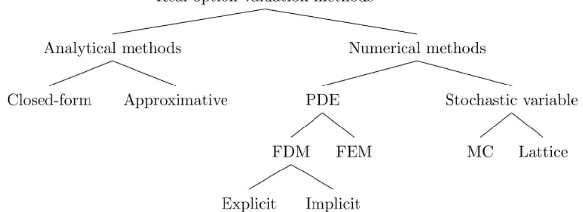
Real option valuation methods can be categorized into two sections - analyt-ical and numeranalyt-ical methods. They can be further divided into subsections as represented in Figure 2.1.
Analytical solutions can divided into two types of solutions – closed-form and approximative solutions. For some problems, such as the infinite horizon investment problem presented in the previous section, a closed-form solution exists. Additional examples of problems that have a closed-form solution are valuation of two risky assets with restricted option to exercise [68], valua-tion of opvalua-tions with possibility to exchange one asset for another [50], [16] and valuation of compound options [31]. In some cases a closed-form solu-tion does not exist but an approximative solusolu-tion with reasonable accuracy can be derived, for example by using polynomial approximations [32], linear
Real option valuation methods Analytical methods Closed-form Approximative Numerical methods PDE FDM Explicit Implicit FEM Stochastic variable MC Lattice
Figure 2.1: Classification of real option valuation methods.
linearpolation [27] or posing restrictions on feasible exercise strategies [6], [41].
However, there are several types of problems for which cannot be solved analytically. Some of the key features that break the solvability with analyti-cal methods, in addition to previously discussed finite horizon, are increasing number of variables and non-constant variables. Needless to say, there are highly important features when modeling the real world. Limiting the num-ber of variables or assuming constant features are major restrictive elements in real options models, which are typically implemented merely for academic reasons or to obtain some solution to problem.
Numerical methods can be used to derive a solution by approximating the underlying stochastic process or partial di↵erential equation (PDE) of the model. Commonly used methods for approximating a stochastic process are Monte Carlo method (MC) and di↵erent types of lattice methods. In Monte Carlo method the possible outcome is simulated by repeated random sam-pling, while in the lattice methods the underlying stochastic process modeled by dividing the process into discrete steps. Monte Carlo method is typically used on relatively simple problems, e.g. real option valuation problems with no possibility to early exercise [9]. Lately the Monte Carlo method has also been used with more complex problems with an early exercise option [15]. Lattice methods, such as binomial and trinomial lattice tree methods, are commonly used in various types of problems due to their intuitive approach and usability [17], and in some cases they are easily extendable [10].
Numerical solution can also be derived by approximating a partial dif-ferential equation of the real option model. This can be done with methods such as finite di↵erence method (FDM) and finite element method (FEM). The underlying idea in both methods is to discretize the solution domain and
calculate an approximative solution of the di↵erential equation in the whole domain. Finite di↵erence method and its two solution schemes, explicit and implicit schemes, are more commonly used within real options theory. Exam-ples of usages vary from using the explicit finite di↵erence method to optimize the cut-o↵ policy of mines [70] to modeling of generalized jump process with implicit finite di↵erence method [12]. Finite element method has not been used that extensively the options theory probably due to its relatively high level of complexity, but there are several examples within financial options, such as combined penalty method for American options [? ] and at least one example within real options theory [2].
Comparing the two real option valuation method approaches used in the corresponding literature, we note that there are three major disadvantages with analytical methods. First, the problem at hand should be simple enough so that an analytical solution can be derived. This widely restricts the prob-lems to a small subset of probprob-lems for which a closed-from solution exists. These problems are rarely an accurate description of reality as several sim-plifying assumption are usually made to obtain an analytical solution, such as assuming infinite horizon, constant risk-free rate or restricting the exercise of an option. This fact cannot be stressed highly enough – in practice it is essentially the same thing as designing an airplane with approximative solu-tions for Navier-Stokes equation describing fluid flow on a wing. Even though the required accuracy with real options is not at the same level, the result would be devastating. Secondly, a considerable amount of work is usually required to work out an analytical solution for even slightly realistic prob-lems. The level of mathematics involved with deriving an analytical solution can be at high level and hence out of reach for common practitioners. In addition, it also takes a considerable amount of time to derive a closed-form solution for some problems that could be solved instantly with numerical methods. Thirdly, the derived analytical solutions are not anymore viable when the complexity of the problem increases. For example, introducing an additional stochastic variable to the model breaks up the analytical solution totally. Consequently, the flexibility of analytical solutions is non-existent. This is a major problem considering the need for minor adjustments and the increasing complexity in the economic world.
Large part of the problems described above can be solved by using numer-ical methods. Numernumer-ical solution can be derived essentially for any type of problem with arbitrary level of complexity. Discretizing a partial di↵erential equation simplifies the problem at hand by definition without neglecting the key items in the model, and the accuracy of the problem can be enhanced by increasing the simulation time, e.g. by choosing more dense grid. Once a numerical method has been implemented, it is very flexible to various types
of minor and major adjustments. For example, the Monte Carlo method is essentially negligible to number of variables and arbitrary type of di↵ er-ential equation can be used with FDM and FEM. In addition, the level of detail numerical methods provide is exhaustive to a single solution provided by analytical methods. Furthermore, the numerical methods are relatively easy for practitioners to use as they can be easily implemented e.g. into a spreadsheet software.
Summarizing, even though analytical methods play a key role in devel-oping the theoretical framework of real options, they are very restricted to simple problems that have merely an academic interest and does not have capabilities to meet the demand of flexibility and ability to model even in-creasing complexity of the real world. In the next chapter we delve more deeply into di↵erent types of numerical methods by presenting the mathe-matical framework behind the methods and introducing two case studies.
Numerical methods
In this chapter we give a short introduction to the most commonly used numerical methods in the field of real options, and present two case studies that we will solve with the numerical methods discussed.
3.1
Introduction
3.1.1
Short history of numerical methods
We noted in the previous chapter that raising the complexity of a real option model even a little bit usually leads to a situation where a solution cannot be derived analytically. This situation is actually quite usual in the world of mathematics. One of the oldest mathematical problems that we can prove to be approximated numerically, was the length of the diagonal in a unit square that was approximated with the Old Babylonian tablet YBC 7289 [28] around 1800 BC. The first person that was credited with the proof was naturally Pythagoras over a millennium later. The same trend has followed throughout the history from linear interpolation to Archimedes’ numerical integration and to Newton’s and Euler method up until the modern days methods of deriving a numerical approximations for complex partial di↵ er-ential equations.
Shortly before the time of computers numerical approximations of func-tions were looked up from gathered tables or calculated by hand one iteration at time. This was a daunting task for some of the mathematical problems, but it was soon to change around the time of the World War II. The Axis powers used the Enigma machine to send encrypted messages to their peers. The Allied forces were puzzled how to break the encryption until pioneering but misunderstood computer scientist Alan Turing developed cipher machines
that were used to break the code1. The cipher machines can be regarded as
first computing machines, so called Turing machines, that led to the invention of the modern computer.
The study of numerical methods exploded with the invention of the mod-ern computer after the World War II. Brilliant minds such as John von Neu-mann devoted part of their precious time to the development of numeri-cal methods, such as the Monte Carlo method and finite di↵erence method (FDM).
The underlying concept behind the Monte Carlo method was used the first time by Enrico Fermi in the 1930s in his study of neutron energies. Around fifteen years later von Neumann alongside with his colleague Stanislaw Ulam formulated the modern version of the Monte Carlo2 method for the study of
nuclear fission at Los Alamos Scientific Laboratory. Thus the Monte Carlo method played a significant role in the Manhattan Project that eventually led to the invention of the first atomic bomb and end of the World War II. [54]
While the concept beneath the FDM dates back to the time of Isaac Newton, the first idea of using FDM in solving problems within the field of physics can be considered to be given in 1928. More rigorous and extended formulations were given by von Neumann, e.g. on the stability conditions of finite di↵erence schemes. The analysis of the finite di↵erence methods broke out thereafter and also other numerical methods gained ground. [69]
3.1.1.1 Numerical methods in real option analysis
Considering the field of real options analysis, several di↵erent numerical methods have been used to obtain a solution for a di↵erential equation that usually arises from the real option analysis. The most commonly used meth-ods are di↵erent types of stochastic simulation methods, lattice methods, and finite di↵erence methods.
In addition to basic usage of the methods, the methods are typically tailored to fit into a specific problem at hand. Some examples of these ex-tensions are stretched trinomial lattices for valuation of public sector R&D investments [74], least-square Monte Carlo method for valuation of power
1Polish mathematician Marian Rejewski was the first one to solve the encryption on
the first versions of the Enigma machine in 1932 by using the permutation and group theory. However, this e↵ort was soon to be fruitless as the Axis powers made continuous improvements to the Enigma machine. [37]
2The name ”Monte Carlo” was suggested by Nicholas Metropolis, a colleague of von
Neumann and Ulam at Los Alamos, according to Ulam’s uncle that would borrow money from his relatives because he ”just had to go to Monte Carlo” [54].
transmission investments [63] and flux-limited upwind scheme for finite dif-ference method to determine the optimal cut-o↵ policy for mines [70]. Fur-thermore, additional numerical methods have been examined for use in real option analysis, such as finite element method [2] which is similar to the finite di↵erence method.
However, in this study we will focus on comparing the basic versions of the three numerical methods most commonly used in real options analysis; the Monte Carlo method, the binomial lattice method and the finite di↵erence method.
3.1.2
Monte Carlo method
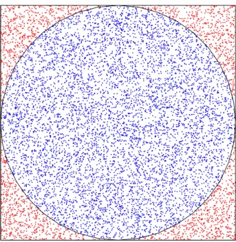
The main idea of the Monte Carlo method is to approximate the probability of some outcome by repeated random sampling. The method as such does not have any rigorous mathematical definition. It is based on the classical definition of probability, which is defined as the number of desired events divided by the number of possible outcomes. These sets of numbers can be regarded as areas or volumes, and distributing a random sampling over the whole domain of possible outcomes ultimately produces the desired outcome. One classic example on the intuition of Monte Carlo method is the esti-mation of ⇡. Suppose we have a circle with radius R inside a square with side length 2R. The ratio between the area of circle and square equals ⇡/4. Thus the estimation for the value of ⇡, which we denote with ˜⇡, can be estimated with the Monte Carlo method by generating random points over the whole domain and counting the number of points N inside the circle and square, that is⇡ ⇡˜⇡= 4Ncircle
Nsquare. See Figure 3.1 for an illustrative simulation.
Clearly as the random sample size approaches infinity, the whole domain will be filled and thus the approximation ˜⇡ !⇡.
The Monte Carlo method is highly convenient in the numerical integration schemes. Consider a simple integral
I = Z
[0,1]d
f(x)dx,
wheref(x) is assumed to be integrable over the defined domain. The integral can be defined with expected value E[f(X)] = I, where X ⇠ unif[0,1]d.
Evaluating the value of the function f(Xi) atn i 1 random points and
gives the Monte Carlo estimate
˜ I = 1 n n X i=1 f(Xi).
Figure 3.1: Monte Carlo simulation for approximating the value of ⇡. Here we used sample size n = 10000 which resulted in ˜⇡ = 3.1356.
Consequently, by the strong law of large numbers3 we note that ˜I ! I as
n ! 1. Thus we obtained an estimate for arbitrary integrable function with the Monte Carlo method. [33]
The increasing sample size is the essence of the Monte Carlo method which ultimately allows the convergence to the exact value. The number of simulations required to obtain a reasonable value can be investigated by examining the rate of convergence. For the Monte Carlo method, the con-vergence rate is obtained from the central limit theorem and it is of order
O(p1
n), wheren denotes the sample size. While this is not the most efficient
rate of convergence in comparison to other numerical integration schemes, the convergence rate holds also in higher dimensions, that is, when d > 1. Thus evaluating integrals in higher dimensions is relatively e↵ortless with the Monte Carlo method as with other deterministic methods the rate of convergence decreases as the dimension increases. [33]
The Monte Carlo method has various applications throughout di↵erent fields due to its applicability to higher dimension problems with uncertainty. It is used heavily in computational physics, chemistry and biology, and in several everyday applications such as weather forecasting and artificial
in-3Strong law of large numbers. Let (X
i :n 1) be independent identically distributed random variables withE|Xi|<1. Then
Pn
i=1Xi
telligence, just to give few examples. Taking into account that the field of finance and economics usually involves expected values, high dimensions and uncertainty, the Monte Carlo method is also highly attractive method for our study.
3.1.3
Binomial lattice model
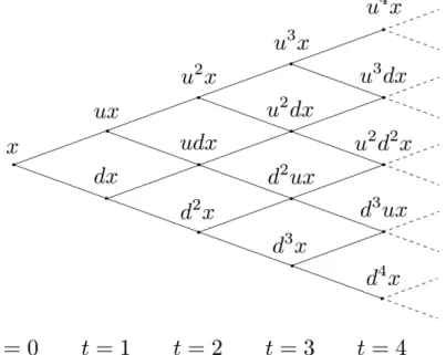
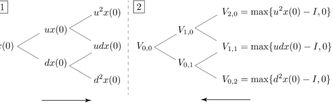
The general idea of behind di↵erent types of lattice models is to simulate the continuous stochastic process of a stochastic variable with discrete steps. This is obtained by dividing the time domain into discrete steps where the value of a stochastic variable is evaluated. In the binomial lattice model the value may go either up or down with a given probability, while in the trinomial lattice model the value has three di↵erent states in the next step. However, in this study we will focus only to the binomial lattice model, see Figure 3.2 for an illustration of the binomial grid. The binomial lattice model was originally introduced by Cox et al. in 1979 [17] as a framework to price options. The model is known as the CRR model in the literature, which abbreviation we will also use.
Figure 3.2: Schematic illustration of a binomial lattice grid where the stochas-tic variable xcan either increase or decrease in the discrete time grid.
Suppose that we have a continuous stochastic processx, which is divided inton i 0 discrete steps. Thus the value of the stochastic variable at each node is given as xi. Advancing from a node forwards, the value can either
increase by the factor u with probability p, or decrease by the factor d < u
with probability (1 p). Let Un denote the number of movements upwards
and thus the movements Un follow Binomial distribution with n trials with
probability p, that isUn⇠B(n, q). Consequently, for the binomial model at
the terminal time i=n, we have
xn =puUndn Un =peUnln(
u
d)+nln(d).
We assume that the probability for the up and down is the same, that is
p= 1 2, and that u=eb t+ p t, d =eb t p t, where we have b= 1 2 ln(u) + ln(d) t , = 1 2 = ln(u) ln(d) p t .
Consequently, with the given assumptions the value of the stochastic variable at the terminal time T =n t is given as
xn=pe
bT+ pT⇣2Un npn ⌘
.
Now, using the central limit theorem4, we note that
xn !pebT+ W(T)=x(T) as n! 1.
Thus with given parameters the terminal value of the binomial model con-verges to the exact value of the continuous stochastic process. [43]
Few remarks about the convergence. Note that we made some assump-tions about the parameters and assumed that we know the terminal value of the stochastic variable. Regarding the convergence of the binomial lat-tice model, it is unrelevant how the probability p is chosen. However, if the stochastic variable is not dependent on the terminal value, the proof pre-sented above does not guarantee the convergence to the exact value. To prove that the binomial lattice method also applies in cases where the value of the stochastic variable is dependent on the whole time domain, more rig-orous methods should be applied. Using Donsker’s Theorem, which is a extension of the central limit theorem, it can be proven that the binomial lattice method converges weakly to the geometric Brownian motion that is
4Central limit theorem (Lindeberg-L`evy). Let (X
i :n 1) be independent identically distributed random variables withE[Xi] =µandV ar[Xi] = 2<
1. Then Pn i=1Xi nµ p n ! N(0, 2) almost surely asn! 1.
the essence of real option models. However, we will not go through the prove here as it is slightly out of the scope of this study. [44]
Note that the binomial lattice model has similarities with the decision tree analysis that was discussed earlier, but it has two distinct di↵erences. First, the shape of the lattice, i.e. the tree, has a fixed symmetry while in decision tree analysis there can be an arbitrary number of outcomes at every branch. Second, the nodes in the lattice describe the current state of a variable that evolves discretely through time. Thus the binomial lattice method only provides information on the value of a stochastic variable and not the decision itself.
The binomial lattice model introduced above takes us one step closer to finite di↵erence method, which can be regarded as an extension of the lattice model.
3.1.4
Finite di
↵
erence method
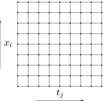
The main idea of finite di↵erence method is to create a discrete grid over the domain of a di↵erential equation, calculate an initial value at some grid point, and move along the grid by calculating an approximation of the derivative at the next grid point. Hence a discrete image of the domain will be formed as all the nodes in the grid are calculated.
Let us start with a simple example. Assume that we are seeking a solution in domainx2[x0, xn] for a first order ordinary di↵erential equation described
by the following set of equations: 8 < : dy dx =f(x, y), y(x0) =y0.
The first step is to form a discrete grid by dividing the continuous domain to non-overlapping intervals. Hence set up a discrete grid x0 < x1 < . . . < xn.
For simplicity, we assume that the grid is regular, that is, the length of interval is given by a constant h and thus xi = x0 +ih, see Figure 3.3 for
illustration.
Next we will start at some initial value and move along the grid to de-termine the discrete image of the domain. There are several interpolation methods to move along the grid. The most simplest is the classical Euler’s method, where the approximation of the di↵erential equation at the neigh-boring grid point is determined from equation
Figure 3.3: Illustration of one dimensional discrete grid.
Hence starting from the initial valuey0, the next grid point can be
calcu-lated according to Equation 3.1. Consequently, moving a single step forwards through the discrete grid until point xn, a numerical approximation of the
di↵erential equation at every grid point can be determined. However, Euler’s method is rarely used in practice as the local and global truncation errors5
are of order O(h2) and O(h), respectively, which imply that the Euler’s
method is rather ine↵ective. However, based on the same single step forward -principle, there other more e↵ective methods available. One example is the fourth order Runge-Kutta method for which the local and global truncation errors are of order O(h5) and O(h4).
Both of the two methods are explicit methods as the approximation of the di↵erential equation is calculated by taking account only the previous value of equation. Contrast to the explicit methods, in implicit methods the current value of the equation is also taken into account. Classical example of an implicit method is the backward Euler method, for which the numerical scheme is the following:
yi+1 =yi+hf(yi+1, xi+1). (3.2)
We note from Equation 3.2 that the state of the system, yi+1, is included on
5The local truncation error measures the error made at a single step, while the global
truncation error measures the sum of local errors for multiple steps. For example in Euler’s method, reducing the step size to a half the local and global discretization errors are reduced by a quarter and half, respectively.
the both sides of the equation, which indicates an implicit method. If the di↵erential equation is linear and an initial value is assigned, it is possible to solve Equation 3.2 from the previous step. However, if the di↵erential equation is nonlinear, it is usually necessary to calculate all the steps to obtain a solution.
As noted in the beginning of this section, there are multiple interpo-lation methods to consider when solving a problem with finite di↵erence method. Considering di↵erential equations outside the illustrative example we presented, the basic idea of finite di↵erence method stays the same as the derivatives of a function are simply replaced with approximations and the discrete values within the grid are calculated one by one. For further details, see for example [49], [23].
3.2
Applications
Next we present two possible applications for the numerical methods dis-cussed above. In the first case we consider an option to invest into a project where the cash flows are uncertain. We assume that the payo↵ from the project will be given at the terminal time when the project is complete. For this type of investment problem a closed-form solution exists, which we will use as a benchmark for the numerical methods. In the second case we con-sider an abandonment option for an ongoing project with uncertainty in cash flows. We assume that project has some salvage value and thus a decision-maker has to decide at every point of time whether to continue the project or abandon the project with a salvage value. Thus the second problem is a optimal stopping problem for which a closed-form solution does not exist and hence numerical methods are required to obtain a solution.
3.2.1
Investment option
Suppose that we are seeking a valuation to a project with a finite lifetimet2
[0, T]. The cash flowsx from the investment are stochastic with a standard deviation . Hence the evolution of cash flows over time are described as
dx(t)
x(t) =rdt+ dW(t), (3.3) whereris the risk-free interest rate. No initial investment is required att= 0, but if the investment to the project is executed it has a fixed investment cost
Consequently, we are dealing with a finite time horizon and thus by follow-ing the discussion in Chapter 2.2 and assumfollow-ing that there are no dividends, the set of equations to be solved are given as
8 > > > < > > > : 1 2 2x2@2V(x, t) @x2 +rx @V(x, t) @x rV(x, t) = @V(x, t) @t , V(0, t) = 0, V(x, T) = max{x I,0}. (3.4a) (3.4b) (3.4c) The first boundary condition (3.4b) is a typical Dirichlet boundary condi-tion that follows from the properties of the stochastic process for the stochas-tic variablex. The second boundary condition (3.4c) determines the optimal investment strategy at the terminal time – the value of the investment op-tion has no value if the fixed investment costI is greater than the cash flows
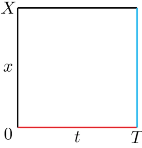
x at the terminal time. The boundary conditions can be visualized on the (x, t)-domain, which is illustrated in Figure 3.4. Note that there are two fixed boundaries, V(x= 0, t) and V(x, t=T), otherwise the boundaries are free. In addition, note that if a solution in the whole domain is calculated, the maximum value for x has to be fixed to some valuex=X.
Figure 3.4: Domain of the case problem, where the fixed boundaries V(x= 0, t) and V(x, t=T) are marked with red and blue color, respectively.
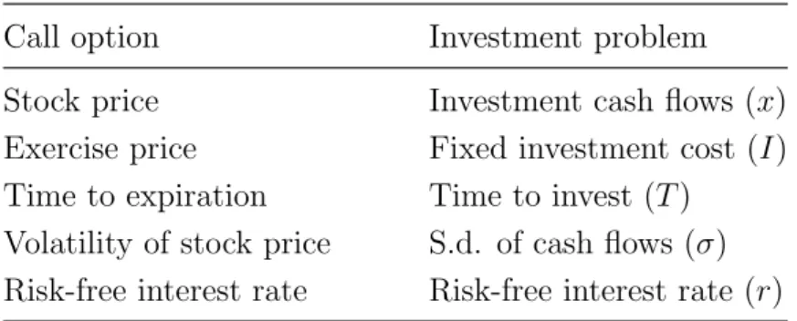
Note that the case study on investment problem described with set of equations (3.4a-3.4c) has a close resemblance to the pricing of an European call option6 with the Black-Scholes equation. The analogies between the two
approaches are listed in Table 3.1.
6In finance, a European option can be exercised only at the expiration time of the
option, while an American option can be exercised at any point of time during the option lifetime. Given the price of underlying security P and the strike priceS, the payo↵for a call option is defined as max{P S,0}and for a put option as max{S P,0}.
![Figure 1.1: Some drawbacks of parameters with the discounted cash flow analysis [55].](https://thumb-us.123doks.com/thumbv2/123dok_us/10975293.2985543/8.892.184.698.330.690/figure-drawbacks-parameters-discounted-cash-flow-analysis.webp)
![Figure 1.2: Example of a decision tree analysis scheme applied to product development project with three possible market states and two possible out-comes for cash flow [19].](https://thumb-us.123doks.com/thumbv2/123dok_us/10975293.2985543/9.892.189.696.200.623/figure-example-decision-analysis-applied-development-possible-possible.webp)