Modeling and Prediction of Disease Processes Subject to Intermittent Observation

(1)

Modeling and Prediction of Disease

Processes Subject to Intermittent

Observation

by

Ying Wu

A thesis

presented to the University of Waterloo in fulfillment of the

thesis requirement for the degree of Doctor of Philosophy

in

Statistics - Biostatistics

Waterloo, Ontario, Canada, 2016

c

(2)

I hereby declare that I am the sole author of this thesis. This is a true copy of the thesis, including any required final revisions, as accepted by my examiners.

(3)

Abstract

This thesis is concerned with statistical modeling and prediction of disease processes sub-ject to intermittent observation. Times of disease progression are interval-censored when progression status is only known at a series of assessment times. This situation arises rou-tinely in clinical trials and cohort studies when events of interest are only detectable upon imaging, based on blood tests, or upon careful clinical examination. The work that follows is motivated by the study of demographic, genetic and clinical data available from the University of Toronto Psoriasis Registry and the University of Toronto Psoriatic Arthritis Registry, each involving cohorts of several hundred patients with the respective diseases.

Chapter 2 deals with the problem of selecting important prognostic biomarkers from a large set of candidates biomarkers when the status with respect to an event of interest (e.g. disease progression) is only known at irregularly spaced and individual-specific assess-ment times. Penalized regression techniques (e.g. LASSO, adaptive LASSO and SCAD) are adapted to deal with the interval-censored event times arising from this observation scheme. An expectation-maximization algorithm is developed which is demonstrated to perform well in extensive simulation studies involving independent and correlated contin-uous and binary covariates. Application to the motivating study of the development of arthritis mutilans in patients with psoriatic arthritis is given and several important human leukocyte antigen (HLA) variables are identified for further investigation. Extensions of this algorithm are developed for settings in which data from different sources with dis-tinct disease-related entry conditions are to be synthesized. The extended Turnbull-type expectation-maximization algorithm is based on a complete data likelihood which incorpo-rates missing information from individuals not meeting the entry criteria of the respective registries. Simulation studies demonstrate good empirical performance and an applica-tion to the motivating study identifies HLA markers associated with the onset of psoriatic

(4)

arthritis among individuals with psoriasis. This analysis is carried out using data from a psoriasis registry in which the times to psoriatic arthritis are left-truncated, and psoriatic arthritis registry in which the onset times are right-truncated.

Chapter 3 deals with the challenge of assessing the accuracy of a predictive model when response times are interval-censored. Inverse probability weighted (IPW) and augmented inverse probability weighted (AIPW) estimators of predictive accuracy are developed and evaluated based on the mean prediction error and the area under the receiver operating characteristic curve. The weights are estimated from a multistate model which jointly considers the event process, the inspection process, and the right-censoring processes. We investigate the performance of the proposed methods by simulation and illustrate their application in the context of a motivating rheumatology study in which HLA markers are used for predicting disease progression in psoriatic arthritis.

A two-phase model is developed in Chapter 4 for chronic diseases which feature an indolent phase followed by a phase with more active disease resulting in progression and damage. The time-scales for the intensity functions for the active phase are more naturally based on the time since the start of the active phase, corresponding to a semi-Markov for-mulation. In cohort studies for which the disease status is only known at a series of clinical assessment times, transition times are interval-censored which means the time origin for phase II is interval-censored. Weakly parametric models with piecewise constant baseline hazard and rate functions are specified and an expectation-maximization algorithm is de-scribed for model fitting. A computationally faster two-stage estimation procedure is also developed and the asymptotic variances of the resulting estimators are derived. Simula-tion studies examining the performance of the proposed model show good performance under both maximum likelihood and two-stage estimation. An application to data from the motivating study of disease progression in psoriatic arthritis illustrates the procedure,

(5)

and identifies new human leukocyte antigens associated with the duration of the indolent phase, and others associated with disease progression in the active phase.

(6)

Acknowledgements

Foremost, I would like to express my deepest gratitude to my supervisor Dr. Richard Cook for the continuous support and encouragement of my study and research, for his guidance, patience, valuable insight and advice, immense knowledge and experience. I could not have come this far or even started without his motivation, encouragement and trust in my abilities. I am so grateful to him for bringing great opportunities for me and providing financial support to facilitate my research. I am very lucky and grateful to work with him for the past few years as a student and a research assistant.

I would also like to express my sincere gratitude to my thesis committee. I would like to thank Dr. Jerry Lawless and Dr. Leilei Zeng for their insightful comments and helpful suggestions from the beginning of thesis proposal to the end of defence. I would also like to thank Dr. Thierry Duchesne from University of Laval and Dr. Hossein Abouee-Mehrizi from Department of Management Sciences for taking their time to serve as the external and internal-external member of my thesis committee, for their expertise from different aspects and inspiring questions to perfect my thesis. A very special thanks goes to Dr. Leilei Zeng, for sharing experience in both research and career building, for creating opportunities for collaboration to widen my knowledge.

I must also acknowledge Dr. Dafna Gladman, Dr. Lihi Eder, Dr. Vinod Chandrad and the team from the University of Toronto Psoriatic Arthritis Clinic for the use of the datasets. A very special thanks goes to Ker-Ai Lee, for her encouragement and help in every aspect of my research. Appreciation also goes to Shared Hierarchical Academic Research Computing Network (SHARCNET) and Compute Canada for facilitating the computational work in my thesis.

(7)

and Actuarial Science. In particular I wish to thank Mary Lou Dufton and Marg Feeney for their support and help, as well as all the students in the department for sharing this journey together.

Last but not the least, I would like to thank my friends and family, who are always standing by me and encouraging me to be myself and pursue my passion and dream.

(8)

Dedication

(9)

List of Tables

2.1 Empirical results for interval-censored data with normally distributed

co-variates (p = 100, E(Xij) = 0, V ar(Xij) = 1 and corr(Xij, Xik) = ρ|j−k|,

where ρ = 0.5) summarizing the number of correctly (TP) and incorrectly

(FP) selected variables along with the median and the standard deviation (SD) of the mean squared error (MSE); P-EM denotes analyses based on the proposed penalized EM method and MID denotes analyses based on a pseudo-dataset obtained by mid-point imputation; the tuning parameter is

selected by five-fold cross-validation. . . 23

2.2 Empirical results for interval-censored data with correlated binary

covari-ates (p= 100,E(Xij) = 0.2 and corr(Xij, Xik) = ρ|j−k|if Xij, Xik are in the

same block as discussed in Section 2.3 andρ= 0.2) summarizing the

num-ber of correctly (TP) and incorrectly (FP) selected variables along with the median and the standard deviation (SD) of the mean squared error (MSE); P-EM denotes analyses based on the proposed penalized EM method and MID denotes analyses based on a pseudo-dataset obtained by mid-point

(15)

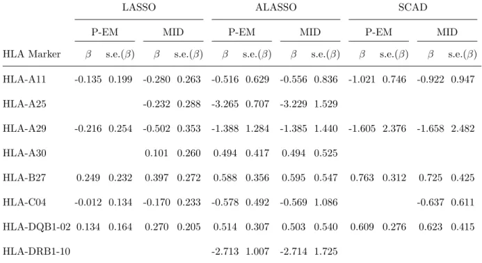
2.3 Selected HLA markers and their effects obtained by variable selection with interval-censored data disease progression data in psoriatic arthritis using

the LASSO, ALASSO and SCAD penalty functions. . . 31

2.4 Empirical results for dataset (33.33% left-truncation and 66.67%

right-truncation) with binary covariates (p = 100, P(Xij = 1) = 0.5)

summa-rizing the number of correctly (TP) and incorrectly (FP) selected variables along with the median and the standard deviation (SD) of the mean squared error (MSE). The tuning parameter is selected by AIC, BIC or CV. Sample

size m= 1200, and nsim= 100 simulations. . . 42

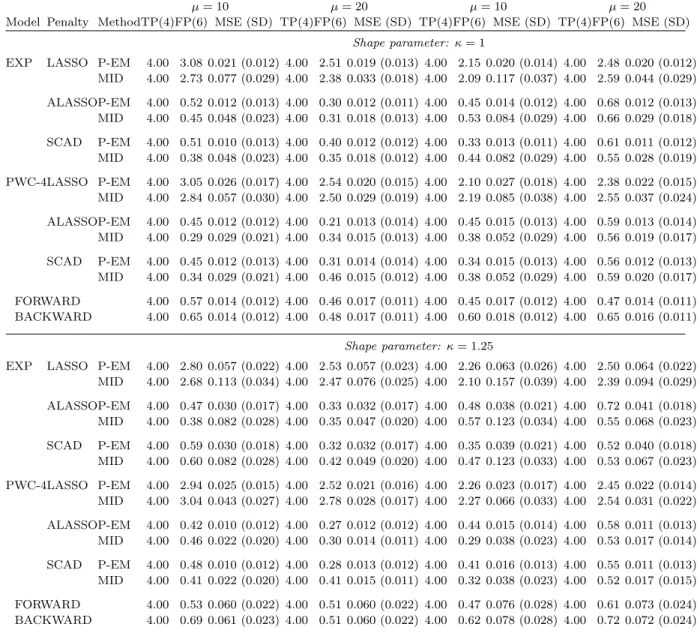
2.A.1 Empirical results for interval-censored data with normally distributed co-variates (p = 10, E(Xij) = 0, V ar(Xij) = 1 and corr(Xij, Xik) = ρ|j−k|)

summarizing the number of correctly (TP) and incorrectly (FP) selected variables along with the median and the standard deviation (SD) of the mean squared error (MSE); P-EM denotes the analyses based on the pro-posed penalized EM method and MID denotes an analysis based on a pseudo-data set obtained by mid-point imputation; the tuning parameter

is selected by five-fold cross validation. . . 48

2.A.2 Empirical results for interval-censored data with correlated binary

covari-ates (p = 10, E(Xij) = 0.2 and corr(Xij, Xik) = ρ|j−k|) summarizing the

number of correctly (TP) and incorrectly (FP) selected variables along with the median and the standard deviation (SD) of the mean squared error (MSE); P-EM denotes the analyses based on the proposed penalized EM method and MID denotes an analysis based on a pseudo-data set obtained by mid-point imputation; the tuning parameter is selected by five-fold cross

(16)

2.B.1 Comparison of three methods of choosing tuning parameter: cross-validation (CV), Bayesian information criterion (BIC) and sparse generalized cross-validation (SGCV). Analyses were based on interval-censored responses with

correlated binary covariates (p= 10) by using proportional hazards models

with a piecewise constant baseline hazards with four pieces (PWC-4) and results are summarized in terms of the number of correctly (TP) and in-correctly (FP) selected variables and the median and standard deviation of

the mean squared error (MSE). . . 53

2.B.2 Comparison of three methods of choosing tuning parameter: cross-validation (CV), Bayesian information criterion (BIC) and sparse generalized cross-validation (SGCV). Analyses were based on interval-censored responses with

multivariate normal covariates (p = 100) by using proportional hazards

models with a piecewise constant baseline hazards with four pieces (PWC-4) and results are summarized in terms of the number of correctly (TP) and incorrectly (FP) selected variables and the median and standard deviation

of the mean squared error (MSE). . . 54

2.C.1 Variance estimation by bootstrap for the simulated dataset with

multi-variate normal comulti-variates and multimulti-variate binary comulti-variates for κ = 1.25,

(17)

3.1 Empirical performance∗ of PE; sample sizem= 500, number of simulations

nsim = 100. The predictor is Yb(X;θ) =b I(P(T > t₀|X;θ)b > 0.5). The

covariates have marginal standard normal distributions. The event time Ti follows a Weibull distribution with rate κλ(λt)κ−1exp (Xi1β1+Xi2β2),

where β1 = log(2), β2 = log(1.5) and κ = 1.25. A time homogeneous

Poisson process is used for the inspection process with rate exp(γ0+Xi1γ1+

Xi3γ2),where γ1 = log(1.1) and γ2 = log(1.5). . . 76

nsim = 100. The predictor is Yb(X;θ) =b I(P(T > t₀|X;θ)b > 0.5). The

covariates are binary with P(Xij = 1) = 0.5, j = 1,2,3. The event time

Ti follows a Weibull distribution with rate κλ(λt)κ−1exp (Xi1β1+Xi2β2),

where β1 = log(2), β2 = log(1.5) and κ = 1.25. A time homogeneous

Poisson process is used for the inspection process with rate exp(γ0+Xi1γ1+

Xi3γ2),where γ1 = log(2) and γ2 = log(2.5). . . 77

nsim= 100. The inspection process is generated by a renewal process. The

gap times between two consecutive inspections are generated by a Gamma

distribution with shape η and rate exp(γ0 +Xi1γ1 +Xi3γ2) , where γ1 =

log(1.1), γ2 = log(1.5) and η= 1.25, 1.5 and 2. (Normal Cases, Xi2 ⊥Xi3) 79

(18)

distribution with shape η and rate exp(γ0 +Xi1γ1 +Xi3γ2), where γ1 =

log(2), γ2 = log(2.5) andη= 1.25, 1.5 and 2. (Binary Cases,Xi2 ⊥Xi3) . 81

log(2), γ2 = log(2.5) andη= 1.25, 1.5 and 2. (Binary Cases,Xi2 6⊥Xi3) . 82

4.1 Empirical performance† of estimators; sample size m = 500, number of

simulations nsim = 500, α1 = 0.036, α2 = 0.5, β1 = (0.5,0.5), β2 =

(₋0.5,−0.5); ASE are average of standard errors estimated via methods in

Section 4.3.3 (EM-MLE) and Section 4.4.2 (EM-TS). . . 108

4.2 Results of fitting piecewise constant baseline hazard model for the duration

of the indolent period and piecewise constant baseline rate model for the occurrence of joint damages under simultaneous (EM-MLE) and two-stage

(EM-TW) estimation; p₋values are based on Wald tests. . . 111

4.A.1 Pseudo-dataframe for the maximization of Q1. . . 116

(19)

List of Figures

1.1 Lexis diagram of event and assessment times on the scale of calendar time

(horizontal axis) and the time since initiating event (the vertical axis). . . 3

2.1 Plots of the estimated cumulative distribution functions for the time from

psoriatic arthritis diagnosis and clinic entry (Kaplan-Meier estimate) and the times between radiological assessments based on a semi-Markov model with a gamma frailty (panel (a)) and the Turnbull estimate with a pointwise 95% confidence band for the marginal cumulative distribution function of

the time from disease onset to arthritis mutilans (panel (b)). . . 13

2.2 Box plots of the error for the estimated regression coefficients βb_k−β_k, k =

5,22,95,96, for each penalty function for datasets with correlated binary

covariates (p= 100) with κ= 1.25, µ= 20. . . 27

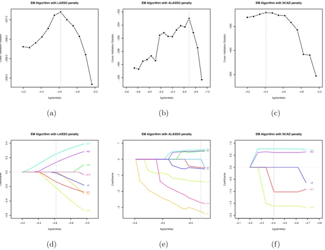
2.3 Plots of the cross validation statistics and shrinkage of coefficients in the

PsA dataset based on piecewise constant hazard model via EM algorithm

(20)

2.4 Lexis diagrams of the calendar times of birth (B), onset of psoriasis (E0)

and onset of psoriatic arthritis (E1), along with screening times (A0) for

UTPC (left panel) and the UTPAC (right panel). . . 36

2.5 Plots of the BIC (1st column), 5-fold cross-validation statistic (2nd column)

and shrinkage estimates of coefficients (3rd column) against the tuning pa-rameter from penalized regression of the PsA dataset based on a piece-wise constant hazard model (PWC-4) fitted via an EM algorithm with the LASSO, ALASSO or SCAD penalty. The fixed covariates are gender and

the onset age of psoriasis. . . 44

2.A.1 Box plots of the error for the estimated regression coefficients βb_k − β_k,

k = 1,2,3,5, for each penalty function for datasets with correlated binary

covariates (p= 10) with κ= 1.25, µ= 10,ρ= 0.3. . . 50

3.1 A multistate diagram for joint consideration of event, random drop-out and

assessment times. . . 67

3.2 Four schematic diagram enumerating possible combinations of (Y,∆); the

solid lines denote observations in which the event status is known att0 and

the dashed lines denote individual whose event status cannot be classified and hence who are excluded from the sum in (3.13); the solid dots denote

(21)

3.3 Plots of the estimates of the prediction error againstt0 with a binary

predic-tor I(P(T > t0) >0.5) for the models obtained from penalized regression

with the LASSO, ALASSO and SCAD penalty functions. The upper panels show estimates obtained by using unweighted, inverse probability weighted and augmented inverse weighted methods; the bottom panels show

esti-mates obtained by using model- and imputation-based methods. . . 86

3.4 Plots of the estimates of the AUC againstt0with a binary predictorI(P(T >

t0) > c), where c ranging from 0 to 1. The response models are obtained

from penalized regression with the LASSO, ALASSO and SCAD penalty

functions. . . 87

3.5 Estimates of ROC curves at t0 =10, 20 and 30 years by inverse probability

weighted (upper panels) and augmented inverse probability (bottom panels) methods for the models obtained from penalized regression with the LASSO, ALASSO and SCAD penalties with the tuning parameter selected by the

5-fold CV. . . 88

4.1 Plot of assessment times (hatch marks) and time of radiological damaged

joints detected between assessments (solid points) from onset of psoriatic arthritis for a selected sample of patients from University of Toronto Pso-riatic Arthritis Clinic. The dashed line denotes time from disease onset to first occurrence of joint damage, and the solid line denotes the period of

disease progression following onset of damage. . . 93

4.2 Lexis diagram of event and assessment times on the scale of disease duration

(t) on the horizontal axis and the time since start of phase II (t∗_{) on the}

(22)

4.3 Estimates of the probability of having at least one damaged joint as mea-sured from the time since disease onset (left panel) and the expected number

of damaged joints for the time since disease onset (right panel). . . 112

5.1 Multistate diagram illustrating the course of disease in psoriatic arthritis

cohort. . . 122

(23)

Chapter 1 Introduction

1.1 Motivating Research Program

1.1.1 Overview

This research is directed at the development of innovative statistical models and methods to address challenging problems arising in research at the Centre for Prognosis Studies in Rheumatic Diseases at the Toronto Western Hospital. This centre created the Univer-sity of Toronto Psoriasis Clinic (UTPC) in 2008 to study the course of psoriasis (Ps), a

chronic inflammatory skin condition which affects up to 3% of the population (Sch¨afer,

2006). Screened patients identified as having psoriasis are recruited to this clinical registry and upon entry they undergo a detailed clinical examination, provide samples for genetic testing, are then followed prospectively according to a standardized protocol; clinical as-sessments are planned to take place every 6-12 months, but ultimately there is considerable variation in the times of the follow-up assessments.

(24)

Approximately 30% of psoriasis patients develop psoriatic arthritis (PsA), a rheuma-tological disorder featuring inflammatory psoriatic disease as well as inflammation and damage in and around the joints of several areas including the wrists, hands, knees, an-kles, lower back, and neck (Chandran et al., 2010). The University of Toronto Psoriatic Arthritis Clinic (UTPAC) was launched in 1977 to study this complex disease (Gladman et al., 2008). While patients are recruited to this registry for a variety of reasons, a pri-mary method is through the use of a population-based screening tool in the form of a 10 item questionnaire (Tom et al., 2015). Individuals suspected of having psoriatic arthritis based on this tool are invited to attend the clinic for a more definitive diagnosis, and those found to have the disease are invited to join the UTPAC. Upon entry to UTPAC, as in the UTPC, a detailed history is taken, patients undergo a thorough clinical and radiologi-cal examination, and samples are collected for genetic testing. The genotypes of HLA-A, HLA-B, HLA-C, HLA-DR and HLA-DQ alleles were collected in both cohorts. Patients are then scheduled to undergo detailed annual clinical examinations and biannual radiological examinations.

1.1.2 Psoriasis and Psoriatic Arthritis

Patients with psoriasis which is uncomplicated with arthritis (PsC) at the screening time were recruited into the University of Toronto Psoriasis Cohort. To date, it has enrolled several hundred patients, but the analyses reported here are based on data from 580 pa-tients in the registry as of 2013; there are 250 women and 330 men. The age at clinic entry has a mean of 46.4 and standard deviation 13.5 years. The median time from clinic entry to the last visit is 1.2 years with maximum of 7.1 years, and the number of visits ranges from 1 to 8 with a median of 2 visits. And the mean (sd) of age of diagnosis of Ps is 30.4

(25)

(16.2) years.

The University of Toronto Psoriatic Arthritis cohort recruited patients with psoriatic arthritis at the screening time, it has over 1000 patients so far. Among the 1215 patients in the registry as of 2013, there are 524 women and 691 men. The mean age at clinic entry is 44.1 years with a standard deviation of 13.0 years. The median time from clinic entry to the last visit is 4.9 years with maximum of 36.7 years, and the number of visits ranges from 1 to 57 with a median of 6 visits. The mean (sd) of age of diagnosis of Ps and PsA is 28.6 (14.7) and 37.2 (13.4) years respectively.

E0 A0 A1 A2 E1 A3 Date of

Initiating Event ScreeningTime Date ofEvent

L

T L R

Calendar Time of Initiating Event

T im e S in c e In it ia t in g E v e n t T- time of event

L: left truncation time

L(R): left (right) endpoint of censoring time

Figure 1.1: Lexis diagram of event and assessment times on the scale of calendar time (horizontal axis) and the time since initiating event (the vertical axis).

Identification of genetic factors putting psoriasis patients at elevated risk of PsA is important as it will enable high risk psoriasis patients to be monitored more closely to

(26)

ensure treatments geared toward the prevention of damage from arthritis are administered in a timely fashion. Such predictive models can also help guide the selection of high risk patients for inclusion in clinical trials of experimental prophylactic treatments. With the increasing availability of large prospective disease registries, scientists studying the course of chronic conditions often have access to multiple data sources, with each source generated based on its own entry conditions. The different entry conditions of the various registries may be explicitly based on the response process of interest, in which case the statistical analysis must recognize the unique truncation schemes. Moreover, intermittent assessment of individuals in the registries can lead to interval-censored times of interest.

Figure 1.1 is a Lexis diagram we introduce to illustrate the point that in the Ps cohort, the time from Ps onset to PsA onset is subject to left-truncation and interval-censoring. In this diagram the onset of Ps is the initiating event and the onset of PsA is the event

of interest. The date of screening and recruitment to the Ps registry is denoted by A0,

and the follow-up assessments are denoted by A1, A2 and A3. Since an individual will only

be recruited to the Ps registry if they are PsA-free then the time _L = A0 −E0 is the

left-truncation time for the time T = E1−E0 of interest. The last PsA-free assessment

and the first assessment after the onset of PsA define the left (L) and right (R) endpoints of the censoring interval respectively. These latter times are depicted on the vertical axis of Figure 1.1. For patients in the PsA registry there are analogous right-truncation conditions which must be addressed. We develop, evaluate and apply methods for variable selection with left- and right-truncated data with event times subject to interval-censoring.

(27)

1.1.3 Arthritis Mutilans

Psoriatic arthritis can be classified into 5 distinct sub-types according to the phenotypic presentations. Arthritis mutilans is considered to be the most severe form of PsA in which patients experience deformity and severe destruction of the joints. While there is no clinical agreement on how to precisely define arthritis mutilans, it represents a state of significant joint damage arising from an extreme form of arthritic component of the disease; here we define it as present if an individual has 5 or more joints with the advanced stage of damage according to the modified Steinbrocker score. It is important to identify clinical predictors and biomarkers for arthritis mutalins in order to prevent further joint destruction. Data from 604 patients in the PsA registry are used in these analyses. A total of 96 HLA markers were used in the study, but 20 of these markers had a frequency in the sample of less than 1% and so were excluded from further consideration, leaving 76 markers to select from. We expand on the description of the problems and approaches in the following subsections.

1.2 General Introduction to Research Topics

The previous section gave a brief overview of the disease processes of interest and the data available for analysis. The following is a similarly brief overview of the types of methodological problems to be considered in the future chapters. A literature review, notation and other details are contained in the respective chapters, which for the most part are self-contained.

(28)

1.2.1 Penalized Regression for Interval-Censored Times of

Dis-ease Progression

In the context of time to event analysis, much of the methodological work on variable selection has been carried out for right-censored data. When events of interest are only detectable upon imaging, as is the case for joint damage which is assessed radiologically at periodic examination times, times of joint damage are interval-censored. Truncation is also often a factor in life history analysis when using data from different registries or other sources, and truncation conditions must be recognized for analyses to be valid.

We propose an algorithm for penalized regression (e.g. LASSO, adaptive LASSO and SCAD) to handle truncated and interval-censored times in Chapter 2. A flexible parametric model with piecewise constant baseline hazard function is adopted and an expectation-maximization algorithm is described which is empirically shown to perform well. The developments are presented in two stages motivated by two distinct problems. We first develop an algorithm dealing with interval-censored responses with a view to identifying markers associated with the development of arthritis mutilans in patients with PsA. Several important human leukocyte antigen (HLA) variables are identified for further investigation.

An extension is then described and evaluated to deal with truncated data using a a penalized Turnbull-type complete data likelihood which incorporates information from individuals who did not satisfy the selection criteria. Simulation studies demonstrate good empirical performance and an application to the motivating study identifies HLA markers associated with the onset of psoriatic arthritis in patients with psoriasis from both the Ps and PsA cohorts. Both left- and right-truncation must be dealt with in analyses using data from both cohorts.

(29)

1.2.2 Assessing the Accuracy of Predictive Models with

Interval-Censored Data

Assessing the statistical performance of a prediction model is important for establishing the validity of a prognostic model and hence in directing medical and clinical decisions. There has been a lot of work directed at the evaluation of predictive models with right-censored data. Methods include estimation of overall prediction error by using loss functions, and evaluation of discriminative ability through use of the receiver operating characteristic (ROC) curves for event status.

In Chapter 3, inverse probability weighted (IPW) and augmented inverse probability weighted (AIPW) estimators are developed and evaluated based on the mean prediction error and the area under the receiver operating characteristic curve to evaluate the per-formance of predictive models for interval-censored response. The weights are estimated through the use of a multistate model facilitating the joint consideration of the event,

inspection and drop-out processes. We empirically investigate the performance of the

proposed methods and illustrate their application in the context of a motivating rheuma-tology study in which HLA markers are used for predicting disease progression in psoriatic arthritis patients.

1.2.3 A Two-Phase Model for Chronic Disease Processes Under

Intermittent Inspection

In many chronic diseases, there is often considerable variation in the course of disease. In rheumatoid arthritis, for example, the length of inactive disease may vary extensively between individuals. Moreover, once the disease becomes “active”, some individuals

(30)

expe-rience rapid progression while others expeexpe-rience minimal disease activity. One approach to deal with this kind of situation is using models with multiple components. In Chapter 4, we propose a two-phase model which has one component for the time from disease occur-rence to the onset of damage, and another component which characterizes the nature of the damage process once it begins. This model can be used to separately examine prognostic factors for the length of the inactive phase as well as factors prognostic for the nature and rate of damage in the active phase. It can therefore be used to obtain a more appropriate representation of a complex multi-phase disease process, can help identify different types of risk factors, and could yield more accurate prediction models.

With interval-censored recurrent event data, all we known are counts of the occurrences of events between assessments. Therefore, the two-phase model involves modeling interval-censored times of the precipitating event (i.e. the first joint to become damaged) and panel count data with a latent time origin. Simulation studies are conducted to examine the performance of the proposed approach to model fitting. Application to data from the motivating study of disease progression in psoriatic arthritis is also given.

(31)

Chapter 2 Penalized Regression for

Interval-Censored Times of Disease

Progression

2.1 Introduction

2.1.1 Variable Selection and Penalized Regression

The literature on statistical methods for variable selection has developed considerably over the last twenty years. Breiman (1996) pointed out that the traditional method of best subset selection was unstable and that this instability could lead to poor performance regarding prediction. While ridge regression (Hoerl and Kennard, 1970) imposes some shrinkage which leads to more stable models, it does not set any coefficients to zero and therefore does not “select” key variables. Tibshirani (1996) proposed a “least absolute

(32)

shrinkage and selection operator”, widely known by the acronym “LASSO”. The LASSO attempts to maintain the advantages of both subset selection and ridge regression by shrinking some coefficients and setting other coefficients to zero through the addition of a particular penalty function to the log-likelihood. Several other penalty functions have been developed and studied over the last decade to cope with high dimensional predictor spaces, including the smoothly-clipped absolute deviation (SCAD) (Fan and Li, 2001; Zou and Li, 2008), the adaptive LASSO (Zou, 2006), the elastic net (Zou and Hastie, 2005), the grouped LASSO (Yuan and Lin, 2005), the fused LASSO (Tibshirani et al., 2005) and the minimax concave penalty (MCP) (Zhang, 2010).

While much of the work on variable selection techniques was initially carried out in the context of continuous responses (Tibshirani, 1996; Fan and Li, 2001; Zou, 2006), advances have been made to deal with binary responses (Park and Hastie, 2007; Friedman et al., 2010) and time to event responses (Tibshirani, 1997; Fan and Li, 2002; Zhang and Lu, 2007). For the latter, the penalty term is typically applied to the partial likelihood (Cox, 1975) arising from a semiparametric Cox regression model (Cox, 1972) when data are right-censored.

Witten and Tibshirani (2009) give an excellent overview of the challenges arising with particularly high dimensional covariate data in settings with censored outcomes and provide an extensive discussion of the specific objectives one might have in particular scientific contexts; another useful account can be found in Li and Ma (2013). The inherent difficulty in obtaining robust and generalizable findings from samples with censored responses and high dimensional covariates is evident from the inconsistency of findings across seemingly similar patient populations and the modest gains that have been made despite considerable advances in biotechnology and statistical methods (McShane et al., 2005a). The limitations analysts face due to inadequate sample size of individual studies (Polley et al., 2013) and

(33)

the inconsistency of findings across studies has led to an increased interest in synthesizing findings over multiple studies. Assimilating information from several sources can be helpful, but it is important to clearly understand the differences between the frameworks and goals of the studies contributing to this synthesis. Guidelines have been developed for reporting findings from biomarker studies with this in mind, which advocate clear statements of study objectives, study design, methods of processing samples, and the approach to statistical analysis (McShane et al., 2005b; Altman et al., 2012).

Many prospective studies, however, have the added complication that the event times of interest are subject to interval-censoring. In clinical trials involving cancer patients at risk of metastases, for example, new lesions are only detectable when imaging assessments are carried out (Hortobagyi et al., 1996), and the precise time from randomization to the development of a new lesion is unavailable. In patients infected with cytomegalovirus, the time from infection to viral shedding in the blood is only known to lie between the last negative and first positive serum sample (Betensky and Finkelstein, 1999; Cook et al., 2008). Vertebral fractures in patients with osteoporosis are often asymptomatic, and their occurrence is only detected upon a radiographic examination yielding evidence of a new fracture (Riggs et al., 1990). Sun (2006) gives an excellent account of statistical methods for parametric and semiparametric analysis of interval-censored failure time data.

We consider the problem of variable selection in the context of interval-censored time to event data. We adopt a flexible piecewise exponential model (Friedman, 1982) for the event of interest and penalize the complete data likelihood constructed by treating the interval-censored failure times as known. An expectation-maximization (EM) algorithm (Dempster et al., 1977) is then used for variable selection through optimization of the penalized observed data likelihood. The LASSO, adaptive LASSO and SCAD penalty functions are considered.

(34)

The remainder of this chapter is organized as follows. In Section 2.1.2 we describe the motivating study with the goal of identifying key human leukocyte antigens associated with the development of arthritis mutilans in a cohort of individuals with psoriatic arthri-tis. In Section 2.2 we describe a penalized expectation-maximization algorithm based on a piecewise exponential response model, for which existing techniques for variable selection can be exploited to handle interval-censored event times. This is the primary contribution of this chapter. Simulation studies involving multivariate normal covariates vectors are reported in Section 2.3, which demonstrate superior performance of the proposed method over analyses based on mid-point imputation (Lindsey and Ryan, 1998). Additional

sim-ulation studies for correlated binary covariates are described in Appendix 2.A and studies

of different criteria for selection of tuning parameters (Bradic et al., 2011) are given in

Ap-pendix 2.B. The data from the psoriatic arthritis clinic are analyzed in Section 2.4 using a

variety of penalty functions, and concluding remarks are given in Section 2.5. An extension of this algorithm is described and evaluated to deal with truncated data in Section 2.6.

2.1.2 Prognostic HLA Markers in Psoriatic Arthritis

The University of Toronto Psoriatic Arthritis Clinic is a tertiary referral center for individ-uals with psoriatic arthritis (PsA), an immunological condition which features both skin and joint involvement (Chandran et al., 2010). A registry was created in 1976, which has been recruiting and following patients continuously since its inception, making it one of the largest cohorts of patients with PsA in the world.

Patients undergo a detailed clinical and radiological examination upon entry to the clinic, and provide serum samples for genetic testing. Follow-up clinical and radiological assessments are scheduled annually and every two years respectively in order to track

(35)

changes in joint damage. At each radiological assessment the degree of damage is recorded in sixty-four joints on a five-point scale (Rahman et al., 1998). Arthritis mutilans is a particularly aggressive form of arthritis characterized here by five or more joints with the highest grade of damage. Identification of genetic features associated with this aggressive form of arthritis is important to help identify patients warranting prophylactic treatment with more effective but costly anti-TNF therapy (Kyle et al., 2005) and to help guide the selection of high risk patients for inclusion in clinical trials of experimental treatments. The aim of the current analysis is to identify key human leukocyte antigens which are associated with increased risk of arthritis mutilans in this cohort of patients.

0 10 20 30 40 0.0 0.2 0.4 0.6 0.8 1.0 Diagnosis to 1st X−RAY 1st to 2nd X−RAY 2nd to 3rd X−RAY 3rd to 4th X−RAY 4th to 5th X−RAY 5th to 6th X−RAY 6th to 7th X−RAY 7th to 8th X−RAY 8th to 9th X−RAY 9th to 10th X−RAY TIME IN YEARS CUMULA TIVE PR OBABILITY (a) 0 10 20 30 40 0.0 0.2 0.4 0.6 0.8 1.0

CUMULATIVE PROBABILITY OF ARTHRITIS MUTILANS

YEARS SINCE DIAGNOSIS OF PsA TURNBULL ESTIMATE

POINTWISE 95% CONFIDENCE BAND

(b)

Figure 2.1: Plots of the estimated cumulative distribution functions for the time from psoriatic arthritis diagnosis and clinic entry (Kaplan-Meier estimate) and the times be-tween radiological assessments based on a semi-Markov model with a gamma frailty (panel (a)) and the Turnbull estimate with a pointwise 95% confidence band for the marginal cumulative distribution function of the time from disease onset to arthritis mutilans (panel (b)).

(36)

To date, 1191 patients have been recruited to the University of Toronto Psoriatic Arthri-tis Clinic, and 604 of these have undergone genetic testing to determine their human leuko-cyte antigen profile. A total of 96 human leukoleuko-cyte antigen covariates were available for study but 20 of these markers had a frequency in the sample of less than 1% and so were excluded from further consideration. Among the 604 patients the median time from clinic entry to last radiological assessment is 6.3 years and there is a median of 3 radiological assessments per patient. To give a sense of the variability in the times between radiologi-cal assessments, the estimated cumulative distribution functions of the times between the first 10 radiological assessments are displayed in Figure 2.1a. To account for the between individual variation in the propensity to attend the clinic (or equivalently, to account for the within-individual dependence in the gap times), the estimated cumulative distribution functions were obtained by fitting a semi-Markov model stratified on the cumulative num-ber of radiological assessments and with an individual-specific gamma distributed frailty term (Klein, 1992; Nielsen et al., 1992). The median inter-assessment times range from 2.7 years for the first two or three assessments after clinic entry, to over 6 years for later assessments. Also plotted is a marginal Kaplan-Meier estimate of the time from diagnosis of psoriatic arthritis to clinic entry; the median of this distribution is roughly similar to the median times between assessments but there are more observations in the right tail of this distribution.

Five hundred and seven (83.9%) of the 604 individuals in this dataset were not observed to develop arthritis mutilans and hence provided right-censored times, whereas 97 (16.1%) individuals were known to develop arthritis mutilans and so yielded interval-censored times. Figure 2.1b contains a nonparametric estimate of the cumulative distribution function for the time from disease onset to arthritis mutilans based on the Turnbull algorithm

(37)

steadily increasing risk with roughly 23% developing the condition within 20 years of disease onset.

2.2 Variable Selection with Interval-Censored Data

2.2.1 Notation and the Penalized Complete Data Likelihood

Here we consider the problem of variable selection with interval-censored data. In many settings, including the motivating study, a natural time origin is the time of disease onset.

We let Ti denote the time from disease onset to the event of interest for individual i in a

sample of m independent individuals, i = 1, . . . , m. We assume individuals are examined

at assessment times governed by an independent inspection process (Gr¨uger et al., 1991;

Cook and Lawless, 2014) and let _Ci = [Li, Ri) denote the interval known to contain the

event for subject i, i = 1, . . . , m. For left-censored data Li = 0, for right-censored data

Ri = ∞, and for interval-censored data 0 < Li < Ri < ∞. We let Xi = (Xi1, . . . , Xip)0

denote a p_×1 covariate vector.

We wish to examine the relation between the covariates and the time of interest based

on a proportional hazards model withh(t|Xi;θ) =h0(t;α) exp(Xi0β) whereαparameterizes

the baseline hazard, β = (β1, . . . , βp)0, and θ = (α0, β0)0. We adopt a weakly parametric

piecewise constant baseline hazard function which requires specification of the number and location of times the hazard changes value; we subsequently refer to these as break-points. If 0 =b0 < b1 <· · ·< bK−1 < bK =∞denoteKbreak-points, the baseline hazard function

ish0(s;α) = exp(αk), for s ∈ Bk = [bk−1, bk), k = 1, . . . , K. The survivor function is then F(t_|Xi;θ) = exp{−H(t|Xi;θ)} where H(t|Xi;θ) =

Rt

(38)

vectorXi and an independent inspection process, the observed (partial) likelihood is L(θ)_∝ m Y i=1 {F(Li|Xi;θ)− F(Ri|Xi;θ)}

and the corresponding observed data log-likelihood is

logL(θ)_∝

m X

i=1

log_{F(Li|Xi;θ)− F(Ri|Xi;θ)}. (2.1)

When viewing this as a variable selection problem, we are specifically interested in identifying the component covariates for which the respective regression coefficients are non-zero. Many common methods of variable selection are based on a penalized likelihood of the form

logLPEN(θ) =

1

mlogL(θ)−pγ,λ(β), (2.2)

where the function pγ,λ(β) determines the extent of the penalty for each value of β,

mod-ulated by the tuning parameters (γ, λ). Ridge regression (Hoerl and Kennard, 1970) is

implemented with theL2 penalty pγ,λ(β) =λPp_j₌₁βj2 and the LASSO (Tibshirani, 1996)

uses the L1 penalty pγ,λ(β) = λ

Pp

j=1|βj|; there is no tuning parameter γ in these penalty

functions. The value of the scalar λ is typically found by cross-validation (Shao, 1993)

or generalized cross-validation (Golub et al., 1979). The adaptive LASSO uses adaptively

weighted L1 penalties of the form

pγ,λ(β) = p X

j=1

λj|βj|, (2.3)

with small penalties λj chosen for large coefficients to reduce their shrinkage, and large

penalties for small coefficients to address the selection objective (Zou, 2006). One option is to setλj =λ/|βe_j|, where βe= (βe₁,βe₂, . . . ,βe_p)0 is the maximum likelihood estimate (Zou,

(39)

case, at the (`+ 1)st implementation, λj is set toλ( `)

j =λ/|βe(

`)

j | where βe(`) is obtained on

the `th iteration; when `= 0, we set λ(0)j =λ/|βe_j| as in the first implementation (Fan and

Lv, 2010). We investigate the iterative implementation of the adaptive LASSO in the next section.

The smoothly clipped absolute deviation (SCAD) penalty proposed by Fan and Li (2001) is defined by p0_γ,λ(β) =λ p X j=1 I(_|βj| ≤λ) + (γλ_{− |}βj|)+ (γ−1)λ I(|βj|> λ) ,

whereγ >2 andy+=I(y≥0)×y. This penalty function is continuously differentiable on

(_−∞,0)_∪(0,_∞), but singular at 0 with its derivatives zero outside the range [₋γλ, γλ].

Therefore, the SCAD penalty results in “small” coefficients being set to zero, “moderate” coefficients being shrunk towards zero, and “large” coefficients retained as they are. In principle, the optimal pair (γ, λ) could be obtained using a two-dimensional grid search by cross validation or generalized cross validation. From empirical work, Fan and Li (2001)

suggest γ = 3.7 is a reasonable choice for a variety of problems and we use this in what

follows and selectλ by (generalized) cross validation.

2.2.2 An Expectation-Maximization Algorithm

We develop here an expectation-maximization algorithm for optimizing (2.2) using avail-able algorithms for penalized regression (Dempster et al., 1977). We do this by considering a complete data likelihood in which the latent event time is treated as known rather than interval-censored.

Let Dk(u) = I(u ∈ Bk) denote whether or not the time u is in the interval Bk and

Wk(u) =

Ru

(40)

ti were known, then under the piecewise constant model and given a covariate vector Xi,

the complete data log-likelihood logLCOMP(θ) would be

m X i=1 K X k=1 [Dk(ti){log(ρk) +Xi0β} −Wk(ti)ρkexp(Xi0β)] . (2.4)

LetZik` =I(k=`) indicate k =`,` = 1, . . . , K and let Zik = (Zik1, . . . , ZikK)0 denote the

corresponding vector of these indicator functions, k = 1, . . . , K; thus Zi1 = (1,0, . . . ,0)0,

Zi2 = (0,1, . . . ,0)0, . . ., Zik = (0,0, . . . ,1)0. If αk = logρk for k = 1, . . . , K, and α =

(α1, . . . , αK)0, we can write logLCOMP(θ) = m X i=1 K X k=1 {Dk(ti)Vik0θ−Wk(ti) exp(Vik0θ)} . (2.5)

where Vik = (Zik0 , Xi0)0 and θ = (α0, β0)0. Since the penalty in (2.2) is simply a function of

the regression parameters, maximization of the penalized likelihood (2.2) can be achieved by applying the EM algorithm to the penalized complete data likelihood

1

mlogLCOMP(θ)−pγ,λ(β). (2.6)

The expectation-maximization algorithm proceeds as follows:

The E-step

We let Di = (Li, Ri, Xi) represent the observed data from individual i and D = {Di, i=

1, . . . , m_} denote the observed data for the full sample. The conditional expectation of

(2.6) at the (r+ 1)st iteration is evaluated as

QPEN(θ;θ(r)) =E

logLCOMP(θ)|D;θ(r) −pγ,λ(β), (2.7)

whereθ(r) _{is the estimate obtained from the}_{rth iteration. The required conditional}

expec-tations are therefore∆b

(r)

ik =E[Dk(Ti)|Di;θ(r)] and ωb

(r)

(41)

Let _Cik = Ci ∩ Bk = [Lik, Rik) denote the sub-interval of the censoring interval Ci

contained within _Bk. When Cik = ∅, the required expectations are relatively easy to

compute since, for instance, it is clear that Dk(ti) = 0 and ∆b

(r)

ik = 0. Moreover, if bk< Li,

then it is known that individual i was at risk for the entire interval_Bk soWk(ti) =ωb

(r)

ik =

bk−bk−1, and if Ri < bk−1, then Wk(ti) = ωb

(r)

ik = 0 since they are known to have failed

prior to the start of interval _Bk. If, on the other hand,Cik 6=∅ then we have:

b ∆(_ikr) = F(Lik|Xi;θ (r)₎_{− F}₍_R ik|Xi;θ(r)) F(Li|Xi;θ(r))− F(Ri|Xi;θ(r)) (2.8) b ω(_ikr) = max(Li−bk−1,0) (2.9) + Z min(Ri,bk) max(Li,bk−1) F(s_|Xi;θ(r)) F(Li|Xi;θ(r))− F(Ri|Xi;θ(r)) ds .

Given these results, (2.7) can be written more explicitly as

m X i=1 K X k=1 n b ∆_ik(r)V_ik0θ₋ω_b_ik(r)exp(V_ik0θ)o₋pγ,λ(β). (2.10) The M-step

The objective function (2.10) has the form of a penalized Poisson likelihood (McCullagh

and Nelder, 1989). The value θ(r+1) _{that maximizes (2.10) can therefore be obtained}

using software for penalized Poisson regression by creating a dataset comprised of

pseudo-individuals indexed by (i, k). IfRi ≥bk−1, then at the (r+1)st iteration this dataset should

include a contribution from pseudo-individual (i, k) with pseudo-count ∆b

(r)

ik and offset

logω_b_ik(r); if Ri < bk−1 then no such contribution is required. The function QPEN(θ;θ(r)) is

then maximized with respect toθ using standard software for penalized Poisson regression

(e.g. the glmnet(.) function (R Core Team, 2013; Friedman et al., 2010) or SIS(.) (Fan

(42)

This optimization procedure is repeated iteratively with updated values of (2.8) and (2.9) in (2.10) until the difference between successive estimates becomes small enough to satisfy convergence criterion. In our implementation the iterations were terminated when

max j (|θ (r+1) j −θ (r) j |/|θ (r) j |)< , where= 10−6.

Selection of the Optimal Tuning Parameter λopt

The criterion for selecting the optimalλ is similar to the traditional cross validation. Here

we use G-fold cross validation and so partition the dataset intoG subsamples _S1, . . . ,SG;

we refer to _Sg and S − Sg as the gth test and training sets, g = 1, . . . , G. For the SCAD

penalty we fixed γ = 3.7. For a givenλ, the cross-validation statistic is

d CV(λ) = G X g=1 n logL(θb₋_g(λ))−logL₋_g(θb₋_g(λ)) o . (2.11)

whereL₋g is the observed data likelihood (2.1) for the gth training dataset and θb₋_g(λ) is

the estimate for thegth training data, obtained through the penalized EM algorithm. The

optimalλ maximizesCVd(λ).

Simulation studies reported in Appendix 2.B assess the relative performance of

validation, use of the Bayesian information criterion, and the sparse generalized

cross-validation (Bradic et al., 2011). While it is difficult to make general statements, the

different penalty functions yielded good performance under cross-validation (i.e. good sensitivity for picking up important factors) and small mean squared error (MSE) of the

β parameter estimates, with a slightly higher tendency to claim association when there is

none). Since there is often strong interest in identifying important variables for further study, it is reasonable to place more importance on the sensitivity and MSE criteria and

(43)

so we adopt the standard cross-validation approach to selection of the tuning parameter

in the the following empirical studies; this statistic is also used in the R packageglmnet.

2.3 Design and Interpretation of Simulation Studies

In this section, we report on the results of simulation studies designed to assess the per-formance of the penalized expectation-maximization algorithm for variable selection with

interval-censored data. We consider a sample size of m = 500 to correspond roughly

to the size of the sample in the psoriatic arthritis study. In the first setting, p = 100

and Xi ∼ MVNp(0,Σ) are i.i.d. where the (j, k) element of Σ is Σjk = ρ|j−k|, with

ρ = 0.3 or 0.6 to represent a mild or strong autoregressive dependence respectively,

i= 1,2, . . . , m. The conditional hazard forTi is based on a Weibull regression model where

h(t_|Xi;θ) = κη(ηt)κ−1exp(Xi0β). We set βj = 0.5 for j = 1, . . . ,5 and j = 96, . . . ,100, so

that high values ofXi,1, . . . , Xi,5, Xi,96, . . . , Xi,100 are associated with shorter times to the

event, andβj = 0,j = 6, . . . ,95 so thatTi ⊥(Xi,6, . . . , Xi,95)|Xi,1, . . . , Xi,5, Xi,96, . . . , Xi,100.

The elements of Xi with non-zero coefficients were chosen to give both weak and strong

dependence within the set of important covariates.

We consider a study with follow-up planned over [0,1], where for each of κ = 1.0 and

1.25, we solve for η so that P(Ti <1|Xi = 0;θ) = 0.95. We let Ni denote the number of

assessments for individual i, generated according to a Poisson distribution with mean µ,

truncated to ensure at least one follow-up assessment, given by

P(Ni =n|Ni ≥1;µ) =

µn_exp(₋_µ)

n!{1₋exp(₋µ)} , n= 1, . . . .

The ni inspection times 0 < ai1 < · · · < aini < 1 were then generated uniformly over

(44)

Li = max(aij ·I(aij < ti)) and Ri = min(aij ·I(aij > ti)) respectively. One hundred

datasets were then simulated (nsim= 100) forµ= 10 and 20 respectively.

For each dataset, variable selection was carried out based on the penalized expectation-maximization (P-EM) algorithm of Section 2.2 with the LASSO, adaptive LASSO (ALASSO)

and SCAD penalty (γ = 3.7). For each analysis, 5-fold cross validation was carried out

to select the unknown tuning parameter. Analyses were conducted based on proportional hazards models with a piecewise constant baseline hazards with four pieces where the break-points were chosen to correspond to the quartiles of the baseline survival function.

For comparison with a simple alternative approach, datasets were created by an ad hoc

mid-point imputation approach (Lindsey and Ryan, 1998) in which event times for

individ-uals withRi <∞were taken to bet∗i = (Li+Ri)/2. The resulting datasets were analysed

based on the proportional hazards assumption with piecewise constant baseline hazards with the same break-points as used in the P-EM analyses; the corresponding results are labeled MID. The more traditional methods of variable selection based on forward selec-tion and backward eliminaselec-tion were also considered under the true parametric Weibull

regression model where we used p = 0.10 for inclusion or removal of terms; the R

func-tion survreg (R Core Team, 2013; Therneau, 2013) was used in this case as it handles

(45)

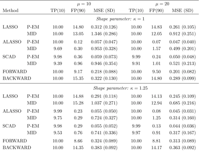
µ= 10 µ= 20

Method TP(10) FP(90) MSE (SD) TP(10) FP(90) MSE (SD)

Shape parameter: κ= 1 LASSO P-EM 10.00 14.80 0.312 (0.126) 10.00 14.83 0.261 (0.105) MID 10.00 13.05 1.346 (0.286) 10.00 12.05 0.912 (0.251) ALASSO P-EM 10.00 0.12 0.057 (0.047) 10.00 0.07 0.047 (0.040) MID 9.69 0.30 0.953 (0.328) 10.00 1.57 0.499 (0.201) SCAD P-EM 9.98 0.36 0.059 (0.073) 9.99 0.24 0.050 (0.048) MID 9.39 0.96 0.946 (0.354) 9.91 1.01 0.521 (0.213) FORWARD 10.00 9.17 0.218 (0.088) 10.00 9.50 0.201 (0.082) BACKWARD 10.00 15.35 0.322 (0.130) 10.00 14.80 0.289 (0.099) Shape parameter: κ= 1.25 LASSO P-EM 10.00 14.88 0.291 (0.118) 10.00 14.13 0.245 (0.109) MID 10.00 15.28 1.037 (0.271) 10.00 12.94 0.685 (0.216) ALASSO P-EM 9.99 0.23 0.055 (0.050) 10.00 0.08 0.045 (0.031) MID 9.75 0.29 0.724 (0.327) 10.00 1.25 0.314 (0.160) SCAD P-EM 9.98 0.29 0.055 (0.052) 9.99 0.13 0.044 (0.036) MID 9.53 0.76 0.741 (0.336) 9.97 0.91 0.317 (0.167) FORWARD 10.00 8.66 0.324 (0.089) 10.00 8.81 0.313 (0.089) BACKWARD 10.00 14.35 0.383 (0.092) 10.00 14.17 0.363 (0.092)

Table 2.1: Empirical results for interval-censored data with normally distributed covariates

(p = 100, E(Xij) = 0, V ar(Xij) = 1 and corr(Xij, Xik) =ρ|j−k|, where ρ = 0.5)

summa-rizing the number of correctly (TP) and incorrectly (FP) selected variables along with the median and the standard deviation (SD) of the mean squared error (MSE); P-EM denotes analyses based on the proposed penalized EM method and MID denotes analyses based on a pseudo-dataset obtained by mid-point imputation; the tuning parameter is selected by five-fold cross-validation.

The number of variables selected was recorded. Among those that are truly associated with the response, the average number selected across all simulated datasets is reported as the mean number of true positive (TP) selections; the correct number of non-zero

(46)

coefficients is given in parentheses in the column headings as TP(10). Among the covariates having no (conditional) association with the event time, the number selected for each dataset was averaged and reported as the mean number of false positive (FP) selections;

the number of truly independent covariates is given in parentheses as FP(90). These

statistics, along with the mean squared error (βb−β)0Σ(βb−β), and the empirical standard

errors of the mean square error, are reported in Table 2.1 based on 100 simulations.

All three penalty functions generally led to selection of the ten covariates associated with the response for the P-EM and MID implementations, with slightly worse performance of the ALASSO and SCAD penalty functions following mid-point imputation. The ALASSO and SCAD penalty functions had the lowest FP values which were lower in the P-EM implementation than following mid-point imputation. For any particular penalty function the mean squared error and the respective standard deviation were always lower when the penalized EM algorithm was used rather than mid-point imputation. These findings point to the advantages of the proposed method which include slightly lower FP values and substantially lower mean squared errors. The forward and backward selection algorithms also featured high FP values. There were little differences between the findings with the

(47)

µ= 10 µ= 20

Method TP(10) FP(90) MSE (SD) TP(10) FP(90) MSE (SD)

Shape parameter: κ= 1 LASSO P-EM 10.00 12.49 0.304 (0.068) 10.00 15.30 0.201 (0.052) MID 10.00 17.64 0.690 (0.117) 10.00 19.01 0.436 (0.086) ALASSO P-EM 9.88 0.82 0.071 (0.067) 9.98 0.26 0.039 (0.033) MID 9.18 0.78 0.491 (0.149) 9.83 0.49 0.255 (0.097) SCAD P-EM 9.94 0.54 0.063 (0.063) 10.00 0.10 0.038 (0.031) MID 9.02 0.96 0.505 (0.166) 9.79 0.40 0.254 (0.102) FORWARD 10.00 11.14 0.244 (0.078) 10.00 11.09 0.183 (0.057) BACKWARD 10.00 15.18 0.299 (0.083) 10.00 14.64 0.231 (0.064) Shape parameter: κ= 1.25 LASSO P-EM 10.00 12.04 0.277 (0.064) 10.00 15.65 0.186 (0.053) MID 9.99 18.15 0.609 (0.100) 10.00 17.91 0.374 (0.074) ALASSO P-EM 9.98 0.59 0.051 (0.042) 10.00 0.22 0.034 (0.023) MID 9.59 0.60 0.404 (0.116) 9.97 0.26 0.186 (0.064) SCAD P-EM 10.00 0.48 0.053 (0.038) 10.00 0.16 0.033 (0.021) MID 9.54 0.93 0.414 (0.118) 9.95 0.42 0.186 (0.064) FORWARD 10.00 10.86 0.198 (0.060) 10.00 10.81 0.180 (0.045) BACKWARD 10.00 14.49 0.233 (0.064) 10.00 13.76 0.195 (0.052)

Table 2.2: Empirical results for interval-censored data with correlated binary covariates

(p = 100, E(Xij) = 0.2 and corr(Xij, Xik) = ρ|j−k| if Xij, Xik are in the same block as

discussed in Section 2.3 and ρ = 0.2) summarizing the number of correctly (TP) and

incorrectly (FP) selected variables along with the median and the standard deviation (SD) of the mean squared error (MSE); P-EM denotes analyses based on the proposed penalized EM method and MID denotes analyses based on a pseudo-dataset obtained by mid-point imputation; the tuning parameter is selected by five-fold cross-validation.

In a second simulation study, we considered correlated binary covariates with p= 100

(48)

study. We set P(Xij = 1) = 0.20, j = 1, . . . ,100. For the dependence structure we

considered the covariates as arising in ten independent blocks such that the correlation

between covariates Xij and Xik within the same block is corr(Xij, Xik) = ρ|j−k| with

ρ= 0.2. Ten covariates were identified to have coefficients equal to one, where these were

chosen to give a combination of pairwise independence as well as weak, moderate and strong associations between important covariates; all other covariate effects were set to zero. The results displayed in Table 2.2 again demonstrate that all methods tend to select the covariates with the non-zero coefficients on average, although the methods based on the adaptive LASSO and SCAD penalties have negligibly lower TP values. As in the previous simulations, the false positive selection rate is lower with the adaptive LASSO and SCAD penalty functions compared to the LASSO as well as the forward and backward selection

algorithms. The respective mean squared errors are always substantially lower in the

penalized EM algorithms compared to the respective implementation following mid-point imputation.

(49)

LASSO ALASSO SCAD −0.75 −0.50 −0.25 0.00 0.25 0.50 0.75 Estimation of β5 = 0 Error ( β ^ 5 − β5 ) IMPUTED P−EM RC (a)

LASSO ALASSO SCAD

−0.75 −0.50 −0.25 0.00 0.25 0.50 0.75 Estimation of β22 = 1 Error ( β ^ 22 − β22 ) (b)

LASSO ALASSO SCAD

−0.75 −0.50 −0.25 0.00 0.25 0.50 0.75 Estimation of β95 = 0 Error ( β ^ 95 − β95 ) (c)

LASSO ALASSO SCAD

−0.75 −0.50 −0.25 0.00 0.25 0.50 0.75 Estimation of β96 = 1 Error ( β ^ 96 − β96 ) (d)

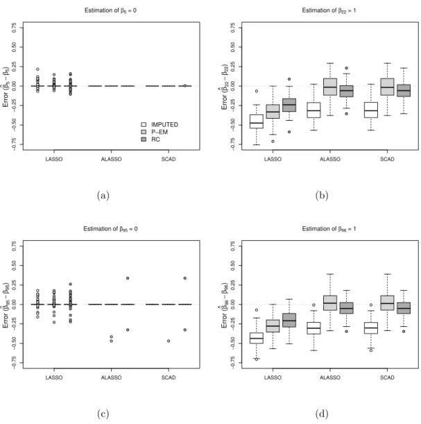
Figure 2.2: Box plots of the error for the estimated regression coefficients βb_k −β_k, k =

5,22,95,96, for each penalty function for datasets with correlated binary covariates (p=

100) with κ= 1.25, µ= 20.

(50)

hundred coefficients in the setting with binary covariates,κ = 1.25, andµ= 20;β5 and β95

(both zero) and β22 andβ96 (both 1.0). For each penalty function the estimates for the

P-EM and MID methods are displayed, along with estimates from an analysis using the true

failure time subject only to administrative right censoring (RC) atC = 1; the latter analysis

is only possible in a simulation study, but is presented for comparison purposes since it provides a natural benchmark for assessing the performance of the proposed algorithm for interval-censored data. It is important to note that different datasets are used for the P-EM, MID and RC analyses, with only the former corresponding to the observed data.

InAppendix 2.A, we present the results of further simulation studies with multivariate

normal and correlated binary covariates when p = 10. Here we consider analyses with

an exponential (time homogeneous) regression model and a piecewise constant baseline hazards (4 pieces) model. The former is included to examine the effect of having a more elaborate (four piece) baseline hazard when a single piece is sufficient as is the case when

κ = 1.0, as well as the effect of gross misspecification of the baseline hazard whenκ= 1.25.

When κ = 1.0 and the P-EM algorithm is used, the PWC-4 model yields a very slightly

higher MSE than was seen for the exponential model, but the results suggest there is little price to pay when the piecewise constant model is used unnecessarily.

When κ = 1.25, the piecewise constant model (PWC-4) had a slightly lower rate of

false positive selections and a lower MSE than the exponential model. A similar study was

conducted with binary covariates (p = 10) with findings that suggest that the adaptive

LASSO and SCAD penalties are again preferable to the LASSO since they generally lead to smaller MSE; among these two methods the relative performance tends to depend on the criteria used (TP, FP or MSE) but they appear broadly comparable overall.

(51)

2.4 HLA Markers and Risk of Arthritis Mutilans

Patients are classified as suffering from arthritis mutilans upon the occurrence of their fifth damaged joint, and interest lies in identifying which among the 76 human leukocyte antigen markers are associated with increased risk of reaching this stage from the time of diagnosis with psoriatic arthritis. The first, second and third quartiles for the closed censoring intervals for the 97 individuals known to have developed arthritis mutilans were 2.50, 8.06 and 15.00 years respectively. These quantiles are much wider than one might expect from a protocol in which radiological assessments are to be scheduled every two years because of the variation between individuals in the propensity to attend the clinic, as well as the potentially long delay from the onset of psoriatic arthritis to clinic entry; see Figure 2.1a. We also remark that the proportion of individuals generating interval-censored times to arthritis mutilans is smaller than that represented in the simulation study, and that the variability in the width of the censoring intervals is considerable; the algorithm can accommodate this setting.

We seek to identify which of the 76 human leukocyte antigens have prognostic value, while controlling for 6 clinical predictors including age at clinic entry, sex, age at onset of psoriasis, age at onset of PsA, family history of psoriasis (yes/no), and family history of psoriatic arthritis (yes/no). We report here on the results of applying the penalized EM algorithm to the interval-censored time of arthritis mutilans among patients in the University of Toronto Psoriatic Arthritis Clinic, using the LASSO, adaptive LASSO and SCAD penalty functions. For comparison purposes, results are also reported based on a right-censored dataset obtained by using midpoint imputation (MID) as examined in the simulation studies. Given the findings from the simulation studies; however, we restrict our attention primarily to the results from the penalized expectation-maximization