Computational Analysis of the Transonic Dynamics Tunnel
Using FUN3D
Pawel Chwalowski
∗,
NASA Langley Research Center, Hampton, VA 23681-2199
Eliot Quon
†,
National Renewable Energy Laboratory (NREL), Golden, CO 80401
Scott E. Brynildsen
‡Vigyan, Inc., Hampton, VA 23666
This paper presents results from an exploratory two-year effort of applying Computational Fluid Dynam-ics (CFD) to analyze the empty-tunnel flow in the NASA Langley Research Center Transonic DynamDynam-ics Tunnel (TDT). The TDT is a continuous-flow, closed circuit, 16- x 16-foot slotted-test-section wind tunnel, with capa-bilities to use air or heavy gas as a working fluid. In this study, experimental data acquired in the empty tunnel using the R-134a test medium was used to calibrate the computational data. The experimental calibration data includes wall pressures, boundary-layer profiles, and the tunnel centerline Mach number profiles. Subsonic and supersonic flow regimes were considered, focusing on Mach 0.5, 0.7 and Mach 1.1 in the TDT test section. This study discusses the computational domain, boundary conditions, and initial conditions selected and the resulting steady-state analyses using NASA’s FUN3D CFD software.
Nomenclature
Roman Symbolsd Deviation distance, inch
Pt Total pressure, psf q Dynamic pressure, psf
Re Reynolds number
Tt Total temperature,◦F
y+ Dimensionless, sublayer-scaled wall coordinate of first node away from surface Acronyms
AePW Aeroelastic Prediction Workshop BTWT Boeing Transonic Wind Tunnel CFD Computational Fluid Dynamics ESP Electronically-Scanned Pressure ETW European Transonic Windtunnel NAS NASA Advanced Supercomputing
∗Aerospace Engineer, Aeroelasticity Branch, Senior AIAA Member
†Post-Doctoral Researcher, AIAA Member ‡Research Engineer, Geolab
NURB Non-Uniform Rational B-spline RANS Reynolds-averaged Navier Stokes RSW Rectangular Supercritical Wing TDT Transonic Dynamics Tunnel
I.
Introduction
I
Na typical wall-mounted wind-tunnel experiment, the tested structure is mounted away from the tunnel’s wall to account for wall interference. The wall interference includes boundary-layer development several feet upstream of the tested structure along the tunnel walls. The distance required to mount the structure away from the tunnel wall is usually well known and carefully incorporated into the test hardware. However, during the test of the Rectangular Supercritical Wing (RSW)1–3in the Transonic Dynamics Tunnel (TDT), the wing was mounted on a splitter plate located only half the desired distance from the wall. During the first Aeroelastic Prediction Workshop (AePW),4–6the workshop participants attempted to calculate pressure distribution on that wing. Several combinations of the compu-tational models were generated to account for the boundary-layer development ahead of the wing, but the calculated surface pressure did not match the experimental data well. Consequently, the idea to create a computational model of the TDT was conceived and initiated in 2012. This paper outlines the steps to generate and test the computational fluid dynamics (CFD) model of the TDT.It is important to emphasize that before any geometry is put into a CFD version of the TDT for computational testing and analysis, the fundamental tunnel calibration quantities obtained in an empty tunnel have to be matched between the experiment and computations. For the TDT, these quantities were obtained during a tunnel calibration experiments conducted in the mid to late 1990s and include wall pressure measurements near the centerline for each of the four walls along the entire test section leg of the tunnel, boundary-layer measurements at six locations, and the centerline Mach number measurements spanning the entire distance of the test section leg of the tunnel.
The TDT, located at NASA Langley Research Center, is a continuous-flow, closed circuit, slotted-test-section wind tunnel with a 16- x 16-foot test section with cropped corners. The tunnel was originally built in 1938, but was converted to the current transonic tunnel in the 1950s, with capabilities to use either air or R-134a heavy gas as a working fluid. In this study, experimental data acquired in the empty tunnel using the R-134a test medium was used to calibrate the computational data. TDT’s unique capabilities are well described and summarized in the recent publication by Ivanco,7where he states the following “Typically regarded as the world’s premier aeroelastic test facility, TDT fulfills a unique niche in the wind tunnel infrastructure as a result of its unparalleled ability to manipulate fluid-structure scaling parameters.”
Much has been published on the topic of wind-tunnel wall interference. Most notably, publications by Krynytzky8–10 defined wall interference issues associated with large transonic wind tunnels, including the TDT and the Boeing Tran-sonic Wind Tunnel (BTWT). He also used CFD analyses9,10to calibrate numerical models against experimental data, which included boundary-layer profiles and test section centerline Mach number distribution and he described slot-flow calculations. In 2004, Glazkow11made an assessment of the slot flow and wall interference for the European Transonic Windtunnel (ETW). More recently, Olander12and Neumann13incorporated wind-tunnel walls in CFD models and ob-tained good comparisons between the computational and experimental data. On the other hand, Massey14incorporated TDT wind-tunnel walls in his rotorcraft research and did not see any influence of the walls on CFD results.
The purpose of this paper is not to offer a replacement of the experimental data with the computational analysis but to show that in some flow regimes, computational methods are mature enough to complement wind-tunnel test-ing, while in other flow regimes, modeling the wind-tunnel flow environment is more difficult and requires further refinement of simulation parameters. The fundamental technical challenges are the size of the computational do-main, the details of the tunnel geometry, and the specification of the boundary conditions. The following statement by Krynytzky10 can be accurately used to describe challenges in computational modeling of the TDT: “Modeling simplifications and choices are still necessary and opportunities for both glory and humiliation abound.”
II.
Computational Model
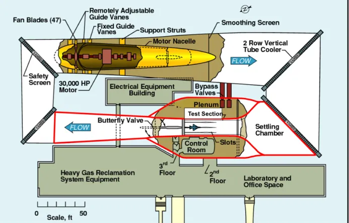
A. Computational GeometryThe plan view of the TDT is shown in Figure1a. The details of the slot locations in the test section leg are identified in Figure1b. Note that in this picture the ‘TS’ stands for tunnel station in dimensions of feet. This means that the ceiling and floor slots begin at tunnel station 50 and end at tunnel station 80. The side-wall slots begin at tunnel station 64 and end at tunnel station 80. Tunnel station 72 coincides with the center of the east wall turntable where the wall-mounted models are installed. The red line in Figure1a around the test section leg of the tunnel shows the outline of the computational domain used in the CFD analysis. The domain begins with the settling chamber and continues into the test section leg, where it is connected with the plenum via slots in all four walls. The domain ends with the diffuser. The shape of the computational domain at the settling chamber is not desirable for the numerical analysis because of the corners where the east and west walls of the chamber meet the turning vanes. However, to include the turning vanes in the computational model together with the rest of the tunnel geometry is too computationally expansive.
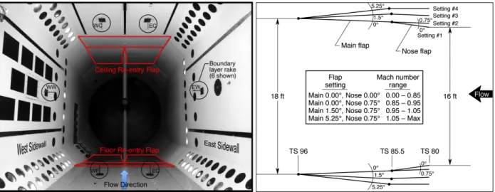
The TDT uses a scheduled system of re-entry flaps in the floor and ceiling just downstream of TS 80 to recapture the working fluid that expands into plenum. As shown in Figure2, the flaps are opened to one of the four predefined positions based on the test section Mach number. The layout of the re-entry flaps is shown in Figure2a. Figure2b identifies the four operational positions.
The approach to obtain the surface geometry of the TDT in this study is ‘as-built’ as opposed to ‘per-drawing’. The same conclusion was reached by Nayani15in his analysis of the NASA Langley’s 14- x 22-ft low-speed wind tunnel. To obtain ‘as-built’ geometry, the Geographic Information Systems (GIS) team at NASA Langley Research Center was contracted to conduct a laser scan of the facility. The laser scan produced a point cloud database, a visual sample of which is shown in Figure3a. The Geometry Laboratory at NASA Langley was provided with that point cloud of approximately 15.5 million laser scanned points. The point cloud data were separated into a few different groups, most notably the different flap settings and the test section leg of the TDT. GeoMagicT M16was then used to create geometry features from the point cloud. Basic features of the tunnel were modeled using best fit algorithms within GeoMagic, including planes for the test section walls, floor, ceiling, and a cone for the diffuser. Other features that cannot be represented by basic geometric shapes were turned into a polygon mesh that GeoMagic then overlaid with non-uniform rational B-spline (NURB) surfaces. Photos of the tunnel were also reviewed to verify any ambiguous point cloud data.
The resulting geometry from GeoMagic was translated into initial graphics exchange specification (IGES) files and moved over to Siemens NXT M17software. Planar surfaces were manipulated to get collinear edges and common intersection vertices where several surfaces meet. NURB surfaces were smoothed over and made to intersect with the remaining geometry in an appropriate way. A nominal 1-inch thickness was applied to the walls of the tunnel away from the scanned surfaces, and a plenum was added based on drawings. The resulting geometry was checked against drawings to ensure that the tunnel features were in the right location or at the proper angle. The final geometry was brought back into GeoMagic to do a point-to-surface comparison to ensure that no large deviations were introduced during the entire process.
Some differences between the drawings and the actual tunnel were captured in the geometry, including angles that are not exactly 90 degrees, distances that are not exactly precise, and areas of wear that have resulted in droops in the floor and other areas of the tunnel. The resulting geometry fits the laser-scanned data with an average deviation of less than 0.4 inches. Figure3b shows estimated deviation distances between the fitted surface and the cloud of points. The areas in red show an estimated deviation of about two inches. This large deviation distance is due to the orientation of the surface with respect to the laser source and the presence of the light-assembly fixtures, which are used to illuminate tunnel test section. The geometric correctness of that part of the tunnel was verified against the drawings. Figure3b also shows some extraneous points obtained in the laser scan, which were ignored in the surface fitting process. B. Computational Mesh
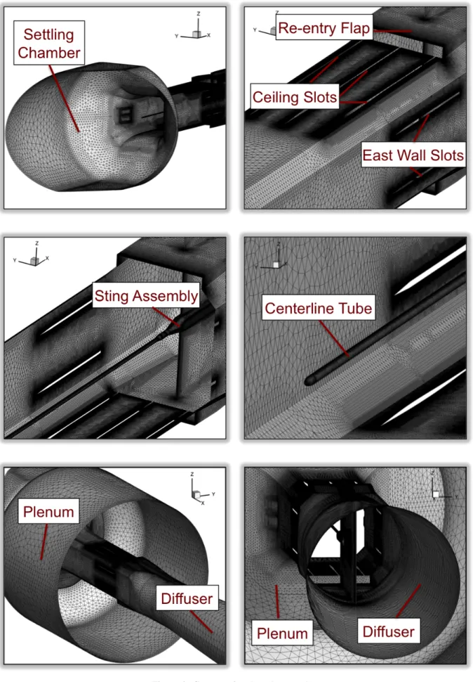
Unstructured tetrahedral grids were used in this study. They were generated using VGRID18 with input prepared using GridTool.19 The tetrahedral elements within the boundary layer were converted into prism elements using preprocessing options within NASA Langley’s FUN3D software.20 First-cell height away from the wall was set to be 9×10⁻⁶feet, which ensured the averagey+<1. The typical mesh size was about 72 million nodes or approximately 400 million elements.
Figure 4shows examples of the mesh used throughout the computational domain. The particular mesh shown corresponds to the fourth re-entry flap setting, used in the computations of the supersonic flow (Mach 1.1) in the test
(a) TDT plan view with computational domain marked in red.
(b) Schematic of TDT showing slots location.
(a) TDT test section with boundary-layer rakes and re-entry flaps outline. (b) Re-entry flaps schedule as a function of Mach number.
Figure 2. Boundary-layer rakes mounted inside the TDT and the layout with operational schedule for the re-entry flaps.
(a) Cloud of points from the laser scan. (b) Estimated deviation distance ‘d’ between fitted surface and the cloud of points.
section. The analysis of the subsonic flow in the test section required a construction of the mesh with the re-entry flap closed.
C. Flow Solver and Solution Process
FUN3D software, which was developed at NASA Langley Research Center, was used in this analysis. FUN3D is a finite-volume unstructured-grid node-based mixed-element RANS flow solver. Various turbulence models are avail-able, but in this study, the turbulence closure was obtained using the Spalart-Allmaras one-equation model. Flux limitation was accomplished with the minmod limiter.21Inviscid fluxes were computed using the Roe flux-difference splitting scheme.22 For the asymptotically-steady cases under consideration, time integration was accomplished by an Euler implicit backwards difference scheme, with local time stepping to accelerate convergence. Most of the steady-state cases in this study were run for about 8000 iterations to achieve an approximate seven order of magnitude drop in residuals.
A total pressure and total temperature boundary condition was used at the inlet. For simplicity in this initial study, the inlet flow angle was assumed to be normal to the inlet plane, even though this flow angle is not accurate since the working fluid enters the test section leg at the angle closer to the turning-vane angle. Future analyses will quantify the effects of flow angle on the computed pressures. At the exit to the computational domain, a back pressure boundary condition was used. The value of this back pressure was iterated to achieve the desired Mach number in the test section. Every computation was run from ‘scratch’ when the back pressure was changed, even for the subsonic flow cases. It was observed that restarting a solution from the previous solution with the change in back pressure resulted in oscillations in the flow field requiring a long time to damp out.
In a typical solution, the flow was initialized to total pressure and total temperature in the settling chamber and to the static pressure elsewhere. This method produced the solution in the shortest amount of time. However, due to the geometric complexity of the computational domain, different methods of flow initialization were tested. These included the initialization of the entire computational domain to either the total pressure and total temperature or to the static pressure. Each steady-state computation took approximately 12 hours on 768 Sandy Bridges cores on the Pleiades computer at NASA’s Advanced Supercomputing (NAS) Division.
The empty-tunnel wall pressure, boundary-layer data, and centerline Mach number experimental data, consisted of static pressure measurements, which were converted into Mach numbers using isentropic flow relations. A similar process was adopted in the computational results. Most of the results in this study, with the exception of boundary-layer data, are presented as Mach numbers computed from the pressure along the length of the test section leg of the tunnel. The boundary-layer data is presented as a velocity ratio of local velocity to freestream velocity plotted in the direction perpendicular to the tunnel walls.
III.
Empty Tunnel Calibration Data
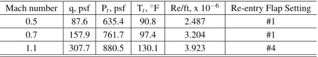
The empty-tunnel experimental calibration data consisted of three sets: boundary-layer profiles, wall pressures, and centerline Mach number data. Since the three experiments were not conducted at the same time, and therefore not at the same exact tunnel conditions, the common denominator in tunnel conditions among the three sets was selected to compare against computations. These tunnel conditions are summarized in Table1.
Table 1. Computational Parameters.
Mach number q, psf Pt, psf Tt,◦F Re/ft, x 10−6 Re-entry Flap Setting
0.5 87.6 635.4 90.8 2.487 #1
0.7 157.9 761.7 97.4 3.204 #1
1.1 307.7 880.5 130.1 3.923 #4
A. Boundary-Layer Calibration
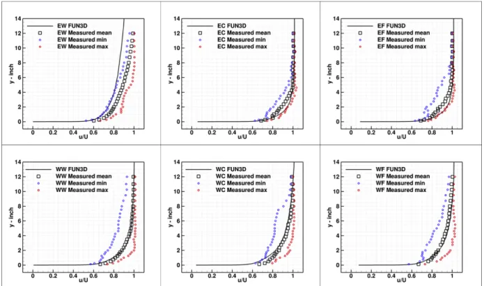
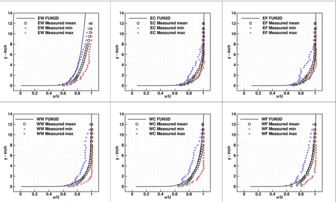
The experimental boundary-layer measurements in the TDT were conducted in 1998 and are documented by Wiese-man.23 Six boundary-layer rakes were mounted at tunnel station 72 to measure the boundary layer in the empty tunnel:
two on the floor, two on the ceiling, one on the east wall and one on the west wall. The locations of the rakes together with their labels are shown in Figure2a. The labels of the rakes are as follows: EW means ‘east wall’, EC means ‘east ceiling’, EF means ‘east floor’, WW means ‘west wall’, WC means ‘west ceiling’, and WF means ‘west floor’. The tubes from the rakes were connected to electronically-scanned pressure (ESP) modules. Boundary-layer profiles were calculated from the measured pressures and the tunnel conditions.
Numerically, the boundary layer was computed by extracting a plane at tunnel station 72 from the solution. A TecplotT M24macro was then used to extract velocity at each rake location. The results are presented in Figures5,6, and7as a velocity ratio plotted in the direction perpendicular to the wall. The experimental data in these figures in-cludes minimum (min), maximum (max), and statistical mean (mean) values of the velocities. The agreement between the experimental and computational data is good considering the flow-angle assumption at the inlet of the computa-tional domain. The most notable differences are observed at the east wall. As previously discussed, the limitations in the computational domain choices upstream of the east wall may affect the computational results. However, in gen-eral, the experimental data also suggests two things. Either the experimental instrumentation used was not adequate for pressure measurements at below atmospheric pressure or the boundary layer in the tunnel exhibits very dynamic behavior. These experimental results suggest the need to repeat the boundary-layer measurement experiment.
Figure 6. Experimental and computational boundary-layer profiles at Mach 0.7.
B. Wall Pressure Calibration
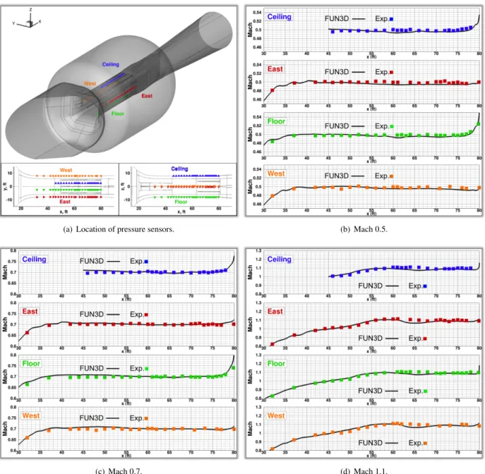
The wall pressure measurements in the TDT were also conducted in 1998 and were documented by Florance.25 In this experiment, the static pressure ports were installed in the test section walls flush with the surface. The floor static ports, labeled in green in Figure8a, were located midway between the floor centerline slot and the east floor slot. The ceiling static ports, labeled in blue in Figure8a, were located midway between the ceiling centerline slot and the west ceiling slot. The east and west wall ports were located in the middle of east and the west walls and are labeled red and orange, respectively, in Figure8a. Mach number from the measured sidewall static pressures was computed using isentropic flow relations.
Computationally, the exact locations of the pressure sensors were known, and the static pressure values were extracted at these locations from the solution. Mach numbers were subsequently computed from these pressure values. The comparisons between the experimentally and computationally obtained Mach numbers are shown in Figure8. The agreement is very good with the largest differences noticed around tunnel station 65 for the Mach 1.1 condition.
(a) Location of pressure sensors. (b) Mach 0.5.
(c) Mach 0.7. (d) Mach 1.1.
Figure 8. TDT wall pressure measurement locations with corresponding experimental and computational Mach number distributions (Mach 0.5, 0.7, and 1.1).
C. Centerline Mach Number Calibration
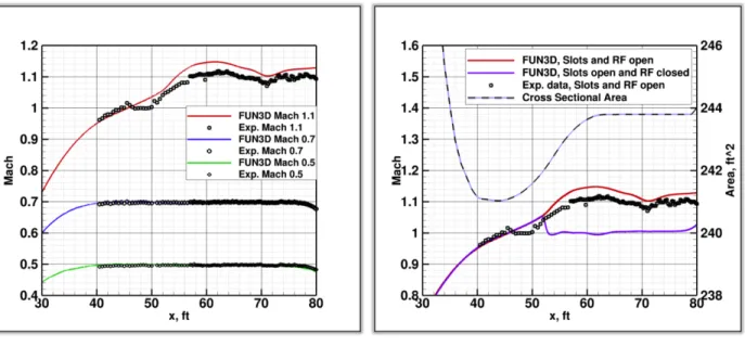
The centerline Mach number experimental data was obtained from Keller.26In this experiment, a 60-foot long 6-inch diameter aluminum tube was installed in the center of the tunnel. The tube, shown in Figure 9, was mounted on the TDT sting/splitter-plate assembly and was also supported by several steel cables along its length. Static pressure sensors on the tube were spaced every six inches between tunnel stations 40 and 56 and every three inches between tunnel stations 58 and 80. As before, the measured static pressures together with tunnel conditions were converted into Mach numbers using isentropic flow equations. Computationally, a Tecplot cutting plane across the tube was used to extract corresponding static pressures. The computational results and the experimental data are compared in Figure10a. There is excellent agreement at both Mach 0.5 and 0.7. However, some discrepancy is present at Mach 1.1. This discrepancy required further analysis and is addressed next.
Figure 10b focuses on Mach 1.1 results. The first consideration is the data between tunnel station 45 and 50, just ahead of the ceiling and floor slots. The experimental data shows a choked flow (Mach number equal 1), with a slight flow acceleration above Mach 1 at tunnel station 45. The computational results do not show choked flow; the flow slightly accelerates through that region, with a distinct flow acceleration near tunnel station 52. The light blue curve with black dashes in Figure10b shows the cross-sectional area of the tunnel between stations 30 and 80. According to the laser scan and the surface fitting process described previously, the minimum cross sectional area in the test section leg of the tunnel is at tunnel station 44. A gradual increase in the cross sectional area is observed between tunnel stations 44 and 62, with nearly a constant area from there up to tunnel station 80. The physical area distribution as opposed to the aerodynamic area supports the computational results. The gradual flow acceleration follows the physical cross-sectional area of the tunnel. One possible explanation of the mismatch in computational and experimental data in this region is that the computational mesh is too coarse to capture the true aerodynamic area. Another possibility is that the laser scan and/or surface fitting through the cloud of points obtained from the laser scan is not correct. It was also suggested that the geometry of the tunnel itself undergoes small changes during the supersonic flow testing, affecting cross-sectional area. In addition, the effects of cables supporting the tube are not accounted for in the computational model. Finally, there is a possibility that the experimental centerline Mach number distribution is affected by the presence of the tube itself. It is difficult to verify this statement since the only source of the experimental data is from the centerline tube experiment. It is possible, however, to remove the tube in the numerical model and examine the centerline Mach number. The results are not shown here, but it appears that the presence of the tube does not affect the centerline Mach number distribution obtained numerically.
The red curve in Figure10b was obtained with both the tunnel slots and the re-entry flaps open (flap setting #4). To verify the computational results at Mach 1.1, the solution with the same boundary conditions, i.e., total pressure and temperature and the static back pressure, was obtained using the mesh with flap setting #1. This means that the slots were left open, but the re-entry flaps were closed. With this check, it was anticipated that the flow would expand and reenter the tunnel through the slots at the same time, resulting in a choked flow with Mach number near 1. The computational result, shown in purple in Figure10b, confirmed this expectation. Corresponding experimental data for this theoretical condition is not available because in the experiment the re-entry flaps are always set to position #4 at Mach 1.1.
(a) Centerline tube: Downstream direction. (b) Centerline tube: Upstream direction.
(a) Mach 0.5, 0.7, and 1.1 plotted together. (b) Mach 1.1 with slots and re-entry flaps (RF) open; Mach 1.1 with slots open and re-entry flaps closed; and tunnel cross sectional area.
Figure 10. Computed and measured centerline Mach numbers at Mach 0.5, 0.7, and 1.1.
IV.
Re-Entry Flap Efficiency and Slot Flow
In this section, the flow through the re-entry flaps and slots is examined more closely. Figure11a shows a compu-tational cross-cutting plane at tunnel station 80. At this station, all slots end, and the re-entry flaps begin. Figure11b offers a zoomed-in view with the axial velocity contours. These contours are adjusted in Figure11c and show in red color the positive (or downstream) axial velocity and in blue color the negative axial velocity. It is estimated that the re-entry flaps efficiency is approximately 80%. This is due to the recirculation region in each corner of the flap, which is shown in Figure11d.
Mach number contours at tunnel station 72 for the three cases considered in this study are shown in Figure12. This figure demonstrates that with the increasing Mach number in the test section the role of the slots to expand the fluid into the TDT plenum increases. The same conclusion can be drawn based on the Mach contours in Figures13,14,15. Figures13and 14show Mach number contours at the plane cutting through the ceiling and floor center slots for the Mach 0.5 and 0.7 cases, respectively. Figure15shows Mach number contours at the plane cutting through the ceiling and floor center slots for the Mach 1.1 case, while Figure16shows the solution for the theoretical Mach 1.1 case with the re-entry flaps closed.
Figure 17shows computationally-predicted flow through the TDT ceiling and east wall slots at Mach 1.1. In Figure17a, the red color represents the flow direction out of the test section through the slots and into the plenum for the Mach 1.1 case that corresponds to the flow shown in Figure15. The blue color represents the opposite flow direction. The CFD analysis predicts flow expansion between tunnel stations 50 and 63 for the ceiling slots and between tunnel stations 70 and 80 for the east wall slots. Similarly, the flow in and out of the test section corresponding to the flow in Figure16is shown in Figure17b. The alternating red and blue colors prove that for this theoretical case (re-entry flaps closed), the flow cannot expand through the slots. Interestingly enough, the east wall slots attempt to expand the flow, but they are too small and too far aft to be efficient.
(a) Axial velocity ‘u’ at tunnel station 80. (b) Axial velocity ‘u’ at tunnel station 80 - zoomed-in.
(c) Axial velocity ‘u’ at tunnel station 80 converted to positive (red) and negative (blue) components.
(d) Re-entry flap corner flow streamlines.
Figure 11. Computational axial velocity at tunnel station 80 and the corner flow for the re-entry flap at Mach 1.1.
Figure 13. Mach number contours across the ceiling and floor center slots at Mach 0.5 case corresponding to the green curve in Figure10a.
Figure 14. Mach number contours across the ceiling and floor center slots at the Mach 0.7 case, corresponding to the blue curve in Figure10a.
Figure 15. Mach number contours across the ceiling and floor center slots at Mach 1.1 case corresponding to the red curve in Figure10b.
Figure 16. Mach number contours across the ceiling and floor center slots at Mach 1.1 case, corresponding to the purple curve in Figure10b.
(a) Flow through the slots at the Mach 1.1 condition, corresponding to the red curve in Figure10b; red and blue colors describe the flow out of and into the test section, respectively.
(b) Flow through the slots at the theoretical Mach 1.1 condition (re-entry flaps closed), corresponding to the purple curve in Figure10b; red and blue colors describe the flow out of and into the test section, respectively.
V.
Concluding Remarks
The objective of this preliminary study was to conduct CFD analysis of the empty TDT and then compare the computed wall pressures, boundary-layer profiles, and centerline Mach number distribution with the experimental data. This objective has been accomplished. However, additional work, both experimental and computational, is required to better understand the flow physics in a large tunnel like the TDT. A recommended list of potential future analysis and calibration experiments is as follows:
• In some instances, the actual shape of the slot edges changes from circular to wedge. However, the computa-tional geometry used in this study assumed a circular shape of the slot edges throughout. A slot edge geometry modification will be incorporated in future analysis.
• The flow angle at the inlet boundary condition (normal to the inlet plane or a turning-vane angle) may have an influence on the boundary-layer profile downstream. A study to compute the flow angle influence is currently in progress.
• The location of the minimum cross-sectional area at tunnel station 44, based on the laser scan, was unexpected. This location was thought to be further downstream. A verification of this finding is necessary by reexamining the laser scan data. At the same time, further resolution of the mesh within the boundary layer is required to compute an effective aerodynamic cross-sectional area.
• It would be beneficial to measure the boundary layer upstream of the slots to eliminate the flow-through-slots effect on the boundary-layer measurements.
• Experimental back pressure measurements in the diffuser would eliminate the necessity of iterating on back pressure in the CFD analysis.
These are just a few examples and thoughts to consider. Future analyses will address the items listed above. In addition, analysis of the TDT with re-entry flap settings #2 and #3 at transonic Mach numbers will be conducted. Of course, the most important question is yet to be answered: Is it possible to model the entire circuit of the tunnel, in-cluding the geometric details of the turning vanes and motor drive, and capture boundary-layer profiles, wall pressures, and centerline Mach number distributions in the test section leg of the tunnel?
Acknowledgments
During this study, the authors consulted with many engineers at NASA. Authors are grateful to Dr. Jan-Renee Carlson and Dr. Bil Kleb for their testing of the internal flow boundary conditions in the FUN3D software. Authors thank Mr. Don Keller, Mr. James Florance, and Ms. Carol Wieseman of the Aeroelasticity Branch for providing centerline Mach number, wall pressures, and boundary-layer experimental data, respectively. Authors also had many fruitful discussions with others colleagues in the Aeroelasticity Branch: Dr. Jennifer Heeg, Dr. Steve Massey, Mr. Tom Ivanco, Dr. Walter Silva, and Ms. Jennifer Pinkerton. Many thanks go to Mr. William Ball and Mr. Jason Hall from the GIS team for conducting the laser scan and to Ms. Norma Farr from the Geolab at NASA for assisting in creating the TDT geometry. We also thank Prof. Marilyn Smith at Georgia Tech for supporting this activity.
References
1Ricketts, R. H., Sandford, M. C., Watson, J. J., and Seidel, D. A., “Geometric and Structural Properties of a Rectangular Supercritical Wing
Oscillated in Pitch for Measurement of Unsteady Trnasonic Pressure Distributions,” NASA TM 1983-85763, Nov. 1983.
2Ricketts, R. H., Sandford, M. C., Seidel, D. A., and Watson, J. J., “Transonic Pressure Distributions on a Rectangular Supercritical Wing
Oscillating in Pitch,” NASA TM 1983-84616, March 1983.
3Bennett, R. M. and Walker, C. E., “Computational Test Cases for a Rectangular Supercritical Wing Undergoing Pitching Oscillations,”
NASA TM 1984-209130, April 1999.
4Heeg, J., Chwalowski, P., Wieseman, C. D., Florence, J. P., and Schuster, D. M., “Lessons learned in the selection and development of test
cases for the Aeroelastic Prediction Workshop: Rectangular Supercritical Wing,” AIAA Paper 2013-0784, Jan. 2013.
5Heeg, J., Chwalowski, P., Schuster, D. M., Dalenbring, M., Jirasek, A., Taylor, P., Mavriplis, D. J., Boucke, A., Ballmann, J., and Smith, M.,
6Heeg, J., Chwalowski, P., Schuster, D. M., and Dalenbring, M., “Overview and lessons learned from the Aeroelastic Prediction Workshop,”
AIAA Paper 2013-1798, April 2013.
7Ivanco, T. G., “Unique Testing Capabilities of the NASA Langley Transonic Dynamics Tunnel, an Exercise in Aeroelastic Scaling,” AIAA
Paper 2013-2625, June 2013.
8Krynytzky, A. J., “Steady-State Wall Interference of a Symmetric Half-Model in the Langley Transonic Dynamics Tunnel,” AIAA Paper
2001-0161, Jan. 2001.
9Krynytzky, A. J. et al., “Uncertainty Evaluation of Wall Interferences in a Large Transonic Wind Tunnel,” AIAA Paper 2010-4341, June
2010.
10Krynytzky, A. J. et al., “Computational Modeling of a Slotted Wall Test Section,” AIAA Paper 2012-2863, June 2012.
11Glazkov, S. A. et al., “Numerical and Experimental Investigations of Slot Flow with Respect to Wind Tunnel Interference Assessment,”
AIAA Paper 2004-2308, June 2004.
12Olander, M., “CFD Simulation of the Volvo Cars Slotted Walls Wind Tunnel,” 2011, CHALMERS UNIVERSITY OF TECHNOLOGY,
G¨oteborg, Sweden.
13Neumann, J. and Mai, H., “Gust response: Simulation of an aeroelastic experiment by a fluid-structure interaction method,”Journal of Fluids and Structures, Vol. 38, April 2013, Pages 290-302.
14Massey, S. J., Kreshock, A. R., and Sekula, M. K., “Coupled CFD/CSD Analysis of an Active-Twist Rotor in a Wind Tunnel with
Experi-mental Validaton,” AHS paper, May 2015, American Helicopter Society 71st Annual Forum Proceedings.
15Nayani, S. N., Sellers, W. L., Brynildsen, S. E., and Everhart, J. L., “Numerical Study of the High-Speed Leg of a Wind Tunnel,” AIAA
Paper 2015-2022, Jan. 2015.
163DSYSTEMS, Rock Hill, SC 29730,GeoMagic, 2013,http://www.3dsystems.com/.
17Siemens, Plano, TX 75024,NX, 2009,http://www.plm.automation.siemens.com/en_us/products/nx/.
18Pirzadeh, S. Z., “Advanced Unstructured Grid Generation for Complex Aerodynamic Applications,” AIAA Paper 2008–7178, Aug. 2008. 19Samareh, J. A., “Unstructured Grids on NURBS Surfaces,” AIAA Paper 1993–3454.
20NASA LaRC, Hampton, VA,FUN3D Manual, Nov. 2015, “http://fun3d.larc.nasa.gov”.
21Roe, P. L., “Characteristic-based schemes for the Euler equations,”Ann. Rev. Fluid Mech., Vol. 18, Pages 337-365.
22Roe, P. L., “Approximate Riemann Solvers, Parameter Vectors, and Difference Schemes,”Journal of Computational Physics, Vol. 43, No.
2, 1981.
23Wieseman, C. D. and Bennett, R. M., “Wall Boundary Layer Measurements for the NASA Langley Transonic Dynamics Tunnel,” NASA
TM 2007-214867, April 2007.
24Tecplot, Bellevue, WA 98015,Tecplot, 2013,http://www.tecplot.com/products/tecplot-360/.
25Florance, J. R. and Rivera, J. A., “Sidewall Mach Number Distributions for the NASA Langley Transonic Dynamics Tunnel,” NASA TM
2001-211019, June 2001.