Aerofoils and Wings for Robustness to Critical
Transition Amplification Factor
Jed Hollom
Department of Mechanical Engineering The University of Sheffield
United Kingdom
Supervisor: Professor N. Qin A thesis submitted for the degree of
Doctor of Philosophy. September 2018
This thesis investigates the use of robust design and optimisation methods to improve nat-ural laminar flow (NLF) aerofoil and wing robustness to variations both in operating condi-tions and uncertainty in surface and flow quality.
NLF is a promising method for aircraft drag reduction but has high sensitivity to operating conditions, flow quality and surface finish. Existing research on this topic has looked to improve NLF designs at a range of operating conditions, but uncertainty in surface and flow quality has not been considered. In this work, surface and flow quality are represented by the critical transition amplification factor, or N-factor, from theeNtransition model. A probabilistic distribution and quantification method for uncertainty in critical N-factor is first selected. This is then used to assess NLF aerofoil performance with uncertainty in critical N-factor. Transition location sensitivity to critical N-factor is found to be linked to transition location sensitivity to lift coefficient; and drag robustness is found to be closely related to transition location robustness.
Robust optimisation is then used to design NLF aerofoils that are insensitive to uncertainty in critical N-factor. This is found to be effective; however, the robustness at off-design flight conditions deteriorates as a result. Many designs with no laminar flow are also generated. These are inherently robust to critical N-factor uncertainty but of no practical use.
A method is then developed that enables the coupling of multi-point and robust optimisa-tion without an increase in computaoptimisa-tional costs. This uses the N-factor envelope fromeN stability analysis to predict transition locations over the critical N-factor range. Multi-point robust optimisation of NLF aerofoils with critical N-factor uncertainty is then carried out. This is able to produce NLF aerofoils with good robustness to critical N-factor uncertainty over a range of lift coefficients and Mach numbers. This envelope sampling method is then extended to account for three-dimensional flows and is used to optimise swept and tapered wing sections for NLF with uncertainty in critical N-factor.
Overall, this work demonstrates that robust design and optimisation method are well suited to the design of NLF aerofoils and wings. Furthermore, it shows that the N-factor envelope fromeN stability analysis can be used to reduce the dimensionality of robust NLF design, making it no more computationally expensive than current multi-point optimisation prob-lems. It therefore makes an original contribution to the field of NLF design and optimisation.
I would first like to thank my supervisor, Professor Ning Qin, for giving me the opportunity to undertake this PhD. Through it, I have been able to expand my knowledge, develop as a person and make many long-lasting friendships.
I would also like to thank Murray Cross for facilitating the link between my PhD and Airbus Commercial Aircraft. This work would not have been possible and would not have been as relevant without the connection to Airbus that Murray provided.
I would like to thank Dr. Stephen Rolston for providing me with the opportunity to spend time at Airbus Group Innovations (AGI) in Bristol. I also appreciate Stephen allowing me to repeatedly extend my stay and for accepting my short notice requests to visit.
I am incredibly grateful to Dr. James Alderman for his advice, support and guidance dur-ing my time at AGI and for the remainder of my PhD. James has been instrumental in the development of this work and I greatly enjoyed our discussions on this and many other topics.
I would also like to thank everyone in the Aeromechanics and Acoustics team at AGI for the warm and friendly working environment they created. It was both a pleasure to spend time there and the most productive period of my studies.
I would like to thank my family for their love and kindness, and the opportunities they have provided me with. I would particularly like to thank them, and Elena Paci, for their support towards the end of my PhD, which carried me through to the finish. I could not have done this without them.
Finally, I would like to thank my peers in the University of Sheffield engineering department and my friends in Sheffield, for making the last few years some of the best.
Nomenclature ix
1 Introduction 1
1.1 Thesis Aim . . . 4
2 Natural Laminar Flow 7 2.1 Flow Transition . . . 7
2.1.1 Flow Stability . . . 8
2.1.2 Primary Instabilities . . . 9
2.1.3 Secondary Instabilities . . . 11
2.1.4 Compressible Flow Stability . . . 12
2.1.5 Receptivity . . . 12
2.2 Transition Modelling . . . 13
2.2.1 Linear Stability Theory . . . 14
2.2.2 eNTransition Model . . . . 15
2.2.3 eNAnalysis of Three-Dimensional Flows . . . . 17
2.2.4 eNModel Calibration . . . . 18
2.2.5 eNModel Coupling to Flow Solvers . . . . 19
2.3 Delaying Transition . . . 20
2.3.1 Design Considerations for NLF . . . 21
2.3.2 Transition Location Robustness . . . 22
2.4 Summary . . . 22
3 Approaches to Aerodynamic Design 25 3.1 Aerodynamic Shape Optimisation . . . 25
3.1.1 Gradient-Based Optimisation . . . 26 3.1.2 Gradient-Free Optimisation . . . 26 3.1.3 Multi-Objective Optimisation . . . 27 3.1.4 Multi-Point Optimisation . . . 29 3.2 Robust Design . . . 29 3.2.1 Uncertainty Analysis . . . 31 3.2.2 Uncertainty Representation . . . 31 3.2.3 Uncertainty Propagation . . . 32
3.3 Application to Natural Laminar Flow . . . 34
3.4 Objectives of this Work . . . 37
4 Tools and Methods 39 4.1 Optimisation Framework . . . 39
4.2 Aerofoil Parametrisation . . . 41
4.3 Computational Solvers . . . 42
4.3.1 Viscous-Inviscid Interaction . . . 43
4.3.2 Subsonic Flow Solver . . . 43
4.3.3 Transonic Flow Solver . . . 46
5 Critical N-factor Uncertainty Analysis 51 5.1 Methodology . . . 51 5.1.1 Uncertainty Representation . . . 51 5.1.2 Uncertainty Propagation . . . 53 5.2 Uncertainty Analysis . . . 54 5.2.1 Aerofoil selection . . . 54 5.2.2 Stochastic Convergence . . . 55 5.3 Subsonic Results . . . 56 5.3.1 Deterministic Performance . . . 56 5.3.2 Stochastic Performance . . . 58
5.3.3 Effect of Uncertainty Standard Deviation . . . 61
5.4 Transonic Results . . . 62
5.4.1 Deterministic Performance . . . 62
5.4.2 Stochastic Performance . . . 64
5.4.3 Effect of Uncertainty Standard Deviation . . . 66
5.5 Summary . . . 66
6 Single-Point Robust Optimisation 69 6.1 Optimisation . . . 69
6.1.1 Problem Formulation . . . 69
6.1.2 Stochastic Convergence . . . 70
6.2 Subsonic Results . . . 71
6.2.1 Design Point Changes . . . 72
6.2.2 Off-Design Analysis . . . 75
6.2.3 Uncertainty Standard Deviation . . . 75
6.3 Transonic Results . . . 76
6.3.1 Design Point Changes . . . 78
6.3.2 Off-Design Analysis . . . 80
6.3.3 Uncertainty Standard Deviation . . . 81
6.4 Summary . . . 82
7 Multi-point Robust Optimisation 85 7.1 Methodology . . . 85
7.1.1 Envelope Sampling Approach . . . 86
7.1.2 Envelope Processing . . . 87
7.2 Optimisation . . . 89
7.2.1 Problem Formulation . . . 89
7.2.2 Validation of the Methodology . . . 90
7.3 Subsonic Results . . . 92
7.3.1 Design Point Changes . . . 94
7.3.2 Performance Polars . . . 96
7.3.3 Sensitivity to Uncertainty Standard Deviation . . . 99
7.4 Transonic Results . . . 100
7.4.1 Design Point Changes . . . 101
7.4.2 Performance Polars . . . 104
7.4.3 Sensitivity to Uncertainty Standard Deviation . . . 105
7.5 Summary . . . 106
8 Extension to Swept Flows 109 8.1 Methodology . . . 109
8.1.1 Calculation of Transition Envelope . . . 110
8.1.2 Key Methodology Assumption . . . 112
8.2 NLF Wing Optimisation . . . 112
8.2.1 Swept Wing Design . . . 112
8.2.2 Problem Formulation . . . 114
8.2.3 Critical N-factor Calibration . . . 115
8.2.4 Validation of the Methodology . . . 117
8.3 High-Sweep Optimisation Results . . . 119
8.3.1 Design Point Changes . . . 122
8.3.2 Additional Validation of the Methodology . . . 126
8.3.3 Span-wise Performance Distribution . . . 127
8.3.4 Sensitivity to Uncertainty Standard Deviation . . . 129
8.4 Low-Sweep Optimisation Results . . . 131
8.4.1 Design Point Changes . . . 134
8.4.2 Additional Validation of the Methodology . . . 137
8.4.3 Span-wise Performance Distribution . . . 139
8.4.4 Sensitivity to Uncertainty Standard Deviation . . . 141
8.5 Summary . . . 142 9 Conclusion 145 9.1 Summary . . . 145 9.2 Key Findings . . . 146 9.3 In Conclusion . . . 148 References 156 Publications 157
Acronyms/Abbreviations
CF Crossflow
CFD Computational Fluid Dynamics HLFC Hybrid Laminar Flow Control LFC Laminar Flow Control
NLF Natural Laminar Flow TS Tollmien-Schlichting
VII Viscous-Inviscid Interaction
Greek
δ Boundary Layer Thickness δ∗ Boundary layer Displacement ∆zte Trailing Edge Thickness
η Crowding Number γ Vorticity Strength Λ Sweep Angle ω Frequency ψ Stream Function σ Source Strength θ Momentum Thickness ε Ellipticity
ξ Stream-wise coordinate
Roman
Cd Drag Coefficient
Cd f Skin Friction Drag Coefficient
Cdp Pressure Drag Coefficient
Cdv Viscous Drag Coefficient
Cdw Wave Drag Coefficient
Cl Lift Coefficient
Nstep Critical N-factor Sample Spacing
Ar Class Shape Transformation Coefficients
C(u) Class Function
Cτ Shear Stress Coefficient
CE Dissipation/Entrainment Coefficient
Cm Moment Coefficient
Fµ(N) Mean Output
Fσ(N) Output Standard Deviation
H Shape Factor
H∗ Kinetic Energy Shape Factor
Hk Kinematic Shape Factor
Hρ Density Shape Factor
hrms Surface Roughness height (Root Mean Square)
km Multi-point Sample Number
kr Robust Sample Number
M Mach Number
M2D Two-dimensional Mach Number
n1/n2 Class Function Exponents
Nσ Critical N-factor Standard Deviation
Ni Ideal Critical N-factor
ni/nt Current/Total Generation Number
Ndv Number of Design Variables
Npop Population Size
P(N) Probability Density Function
r Normal Leading Edge Radius
Re Reynolds Number
Reθ Reynolds number (Momentum Thickness)
S(u) Shape Function
Sre f Wing Area
Tr Transition Location
Tu Turbulent Intensity
u Chord Length Position
W Summation of Weights
zo/zp Original/Perturbationzcoordinate
Subscripts
0 Initial
δ Boundary Layer Thickness
ac Aircraft c f Crossflow cr Critical l Lower Surface le Leading Edge max Maximum
te Trailing Edge
ts Tollmien-Schlichting
u Upper Surface
e Boundary Layer Edge
Introduction
Within the commercial aviation industry, there is a constant demand for reduced fuel con-sumption. This is required to meet the stringent environmental targets set by aviation au-thorities, as well as to reduce running costs for airline operators. Such environmental targets are outlined by the European Commission who specify a 75 percent reduction in CO2and
90 percent reduction in NOxper passenger kilometre by the year 2050 [1].
Throughout aviation history, advancements in aircraft design, engine technology and fuel composition have all resulted in improved aircraft performance. Modern commercial air-craft are highly efficient as a result. However, as the basic configuration of airair-craft has re-mained largely unchanged, each additional design effort produces a diminishing return on improved aircraft efficiency. For this reason, development of new aerodynamic configura-tions and the exploitation of more complex flow phenomena is required for a step change in aircraft performance to be found.
Drag on a transonic commercial transport aircraft can be broken down into individual com-ponents as shown in figure 1.1. Parasite and lift-induced drag make up approximately 94 percent of the total aircraft drag [2, 3]. Lift-induced drag occurs when the lift generated by the wing has a component opposite to the direction of flight. This occurs when a difference in pressure causes flow at the wing-tip to move from the pressure to suction surface, leading to a vortex downstream of the wing-tip and wash over the wing itself. This down-wash induces a change in the local angle of flow over the wing, and so the angle at which lift is generated.
Parasite drag is experienced when an objective moves through a viscous fluid and can be split into skin friction and form drag components. Skin friction accounts for 96 percent of parasite drag, and is the loss of energy due to shear stresses within the boundary layer that forms as a result of flow viscosity. As all wetted areas contribute to this, the fuselage and wing are the largest sources and collectively account for 74 percent of skin friction on an aircraft. Form drag is also due to the formation of the boundary layer, which changes how oncoming flow interacts with the aircraft. Thickening of the boundary layer increases the effective thickness of an aerodynamic body, causing a change in pressure distribution and an increase in drag. This is referred to as form drag. As modern aircraft are highly streamlined, form drag is a small component of parasite drag, contributing only 4 percent.
Parasite Lift-Induced
Wave & Form
Skin Friction
Fusalage Wing Other
Total Drag
Parasite Drag
Skin Friction
Interference 6% 40% 54% 4% 96% 42% 34% 24%
Figure 1.1:Drag breakdown for a typical commercial transport aircraft (data taken from [3])
The other drag sources accounting for approximately 8 percent of total aircraft drag are wave drag and interference drag. Interference drag occurs when flow from different aero-dynamic surfaces mix such that the combined drag is larger than the sum of the individual components. This can occur at junctions between components, where two components are close or if one is behind another [4]. For commercial aircraft, key sources of interference drag are at the intersections between fuselage, wing, pylon and engine. Drag from these sources can, however, be avoided by the inclusion of fairing between components and with careful design, a reduction in drag can instead be obtained [2].
Wave drag is the result of entropy loss through shock waves that can form when there is supersonic flow over an aircraft. This can become a significant component of total drag if strong shock-waves are allowed to form on aerodynamic surfaces such as the wing. Wave drag can, however, be avoided through the use of increased wing sweep, supercritical aero-foil design [5] and shock control methods [6].
There has been extensive research on the reduction of skin friction as it is a significant source of drag. Two approaches to this are possible: turbulent drag reduction and the extension of laminar flow [2, 7]. Turbulent drag reduction attempts to reduce skin friction by modifying turbulent flow features. This has wide applicability as the majority of flow over modern commercial aircraft is turbulent. Such methods include synthetic jets, riblets and large eddy breakup devices [8]. The alternative approach is extension of laminar flow by delaying its transition from laminar to turbulent. As laminar flow can have as much as 90 percent less skin friction drag than turbulent flow [9], and as most flow over modern aircraft is turbulent, there is potential for substantial drag reductions.
Transition from laminar to turbulent flow is due to the growth of small disturbances within the boundary layer flow. If unstable, these instabilities will increase in magnitude until they result in the breakdown of laminarity [10]. Methods available for reducing instability
growth are Laminar Flow Control (LFC), Natural Laminar Flow (NLF) or Hybrid Laminar Flow Control (HLFC).
LFC is the active and continuous modification of the boundary layer through surface cooling or suction [11]; as altering the temperature or velocity profile through the boundary layer is found to have a strong effect on flow stability. LFC is typically associated with boundary layer suction as this has seen more extensive research [9]. NLF makes use of the strong effect pressure gradient has on flow stability. An aerodynamic surface can be designed in such a way as to create the required pressure gradient to dampen boundary layer instabilities. This is considered a passive approach as the pressure gradient is induced naturally during flight. The choice of LFC or NLF depends on the application and flow conditions being experi-enced. LFC is able to provide instability damping where NLF is not effective. Such areas in-clude aircraft fuselage, highly swept wings [11], wings with large chord length and when at high transonic speeds. Where effective, NLF is preferable to LFC as it requires no additional suction or cooling components which increase aircraft weight, manufacturing complexity and cost [2]. Running of a LFC system also requires power which, when siphoned from the propulsion system, reduces aircraft performance. Due to the drawbacks seen with both approaches, a combined Hybrid Laminar Flow Control (HLFC) approach has seen much research. This entails the use of NLF with LFC only where it is not possible to suppress the growth of boundary layer instabilities passively, such as towards the leading edge of highly swept wings. Combining LFC and NLF reduces the suction requirements and complexity of the LFC suction system but also allows for effective instability suppression where not possi-ble with NLF alone. Further developments in LFC and HLFC make use of passive suction, routing the suction chambers to a location on the aircraft with low pressure.
Several major research efforts involving wind tunnel and flight testing of NLF and HLFC have been carried out in Europe. Flight testing of a NLF glove and wind tunnel testing of a half-scale model was carried out by DLR in the late 1980s as part of the national German laminar flow technology programme [12]. This led to the flight test of a second NLF wing glove as part of the European Laminar Flow Investigation (ELFIN) program which began in the early 1990s [13]. Airbus, in partnership with DLR and ONERA, carried out design, wind tunnel and flight testing of HLFC applied to the fin of an A320 test aircraft. This was undertaken in the 1990s and done as part of the Laminar Fin Program [14]. The most recent flight tests were carried out by Airbus in 2017 as part of the Breakthrough Laminar Aircraft Demonstrator in Europe (BLADE) programme, under the European Clean-sky 1 project [15]. This involved the testing of an A340 with NLF outboard wing sections, shown in figure 1.2. Although LFC and HLFC are effective in obtaining extended laminar flow where not possi-ble with NLF, it is still desirapossi-ble to avoid suction-based systems entirely if possipossi-ble. There-fore, aircraft designs exploiting NLF while having low sweep and reduced Mach number have been proposed. Novel aircraft configurations such as those with strut-braced wings also have excellent potential for NLF [17].
While NLF has seen extensive research, laminar flow is often not considered during the design of, and not obtained on, most commercial transport aircraft. One of the main reasons for this is that transition occurs through a number of complex instability mechanisms and is often sensitive to small changes in aerodynamic shape, surface and flow quality and the
Figure 1.2:Airbus BLADE NLF wing section (Photo: P. Pigeyre / Master Films. Copyright: Airbus) [16].
chosen flight conditions [18]. As a result, obtaining extended laminar flow during flight is challenging. Maintaining extended laminar flow over a wide range of operating conditions and at varying surface and flow quality is even harder. For NLF to become viable on modern commercial aircraft, it must be made robust to the factors effecting transition. This requires design at both on and off-design conditions, with consideration for uncertainty in many other input variables.
Research in recent years has, however, indicated that optimisation and robust design meth-ods may be effective at tackling these issues [19–21]. Thanks to increasing computational power, more complex optimisation problems can now be considers. Increasing the dimen-sionality of the design problem, considering multiple design objectives and possible input uncertainties should each help to produce NLF aerofoils and wings with a more consistent performance over a wider range of conditions.
1.1
Thesis Aim
The aim of this work is to investigate the use of robust design and optimisation methods applied to NLF aerofoil and wing design. The goal of this research is to identify means of improving aircraft performance by reducing drag via the extension of NLF while also re-ducing performance sensitivity to changes in operating conditions, flow and surface quality. This is pursued as a lack of robustness to these factors is one of the issues currently limiting the wide-spread use of NLF as a drag reduction method.
Chapter 2 introduces the fields of flow transition, transition modelling and NLF design. Chapter 3 following this provides some background knowledge on optimisation and robust design, and the current state-of-the-art in applying these methods to the development of NLF aerofoils and wings. The current limitations to the practical use of NLF on modern commercial aircraft are then assessed and the specific objective of this study outlined.
Natural Laminar Flow
2.1
Flow Transition
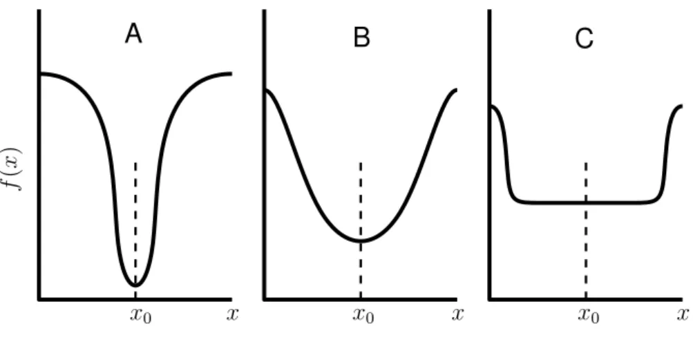
At its fundamental level, flow transition is a result of environmental disturbances entering the boundary layer. These can originate from turbulence within the freestream flow or in-teraction of the flow with surface roughness and irregularities through a process known as receptivity [22]. Flow stability is determined by the growth or decay of these disturbances over time, through space or a combination of both [7]. A flow is stable if disturbances de-cay while an unstable flow results in disturbance growth. Disturbance growth results in the formation of regular oscillations within the boundary layer, referred to as instability waves. The shape and behaviour of each instability wave depends on the amplitude, frequency and phase of the initial flow disturbance [23]. A wide range of disturbance characteristics are possible and result in several different paths to transition. These are shown in figure 2.1.
Environmental Disturbances Receptivity Bypass Turbulence Transient Growth Primary Modes Secondary Mechanisms Breakdown Amplitude A B C D E
For small disturbance amplitudes, path A is taken. The growth of boundary layer insta-bilities is linear and occurs slowly over a large distance. These are referred to as primary instabilities. The continued amplification of primary instabilities results in the creation of secondary instabilities which lead to a rapid breakdown of the flow and the onset of tran-sition [25]. This path to trantran-sition is sometimes referred to as ’Natural Trantran-sition’ [26]. An alternative path to transition occurs when environmental disturbances are large. The devel-opment of primary and secondary instabilities is skipped as turbulent flow features form directly within the laminar boundary layer and result in breakdown of the flow. This is path E, known as bypass transition.
Natural transition and bypass transition both occur when disturbances with an unstable wavelength enter the boundary layer flow. It is also possible for transition to occur when all disturbance frequencies are stable. This is through a process known as transient growth, where stable disturbances interact and see large amplification before decaying. This growth can result in primary instabilities (path B), secondary instabilities (path C) or may be large enough to trigger bypass transition (path D).
Regardless of the path to transition, eventual destabilization and breakdown of the flow is due to the development of what are referred to as ’Emmon spots’ or ’turbulent spots’. Each spot begins with a point-like instability of the laminar flow that grows linearly downstream. Following this is an arrow head shaped region of turbulent flow of smaller scale than the boundary layer height [27]. Breakdown of the flow refers to the initialization and growth of these spots which eventually engulf the entire boundary layer flow.
Natural transition (path A) is of most interest for the development of NLF as disturbance amplitudes are typically small during flight due to low freestream turbulence intensity lev-els [28, 29]. Primary instabilities are also the easiest to model due to their linear behaviour. As transition occurs quickly after non-linear effects occur, the end of this linear region pro-vides a good approximation of the final transition location. The following sections cover different stages of the natural transition process and some of the properties that flow stabil-ity and transition are sensitive to.
2.1.1 Flow Stability
A disturbance wave of a given frequency (ω) at a given Reynolds (Re) number will be in one of three possible states: amplifying, neutral or decaying [30]. Calculating the stability of disturbances with a range of frequencies over a range of Reynolds numbers allows for a neutral stability curve plot to be generated, such as shown in figure 2.2. In both plots, the
xaxis shows Reynolds number based on boundary layer thickness (Reδ), they axis shows
frequency based on boundary layer thickness (ωδ) and the contour lines represent neutral
stability, separating the stable and unstable regions.
Disturbances have a fixed frequency moving downstream, as indicated in figure 2.2b by the horizontal dashed line. Disturbances are initially stable but can encounter an unstable re-gion downstream. Disturbances will normally decay in the stable rere-gion and amplify in the unstable region. However, if amplification through the unstable region is large, secondary instabilities can develop and amplification will continue even on entering the stable re-gion. This will result in a rapid breakdown of the flow to turbulence [30].
Two different forms of the neutral stability curve are typically observed. Figure 2.2a shows a neutral stability curve with an unstable region starting at a low Reynolds number and extending toReδ →∞. Given that the flow is unstable at both low and high Reynolds
num-bers, the instability is not dependent on viscosity and so is considered inviscid. Inviscid instability is directly related to the mean boundary layer velocity profile shape. An inflec-tion point within the velocity profile is found to be a sufficient condiinflec-tion for the flow to be unstable [22]. Free-shear flows, such as jets, wakes and separated flows, and wall bounded flows under an adverse pressure gradient are prone to inviscid instability [28, 30].
Figure 2.2b shows the neutral stability curve for a boundary layer flow with viscous in-stability. In this case, disturbances at all frequencies are damped when Reynolds number is sufficiently large and inertial forces dominate. Thus, viscous forces have a destabilising effect on the flow for a finite Reynolds number range [30]. A flow with viscous instabil-ity can be unstable without an inflection point within the boundary layer velocinstabil-ity profile [30]. Wall-bounded flows have viscous instability when incompressible and under neutral or favourable pressure gradient [28, 30].
Re
δω
δStable
Unstable
Recr
(a)Inviscid instability
Re
δω
δ Stable Unstable ReL ReU (b)Viscous instability Figure 2.2:Example of neutral stability curves for a two-dimensional flow [30].All disturbances are stable and decay below what is referred to as the Critical Reynolds number (Reδ|cr). It would be desirable to keep Reynolds number below this critical value as
disturbances at all frequencies are stable. However, critical Reynolds number is typically of the order ofReδ|cr=O[103]for wall-bound viscous dominated flows and so this is not
pos-sible [28]. A low Reynolds number also causes a boundary layer flow to be less resistant to separation. If this occurs, the resulting free-shear layer is also highly susceptible to inviscid instabilities and can quickly transition [28]. This is an important design consideration for low Reynolds number NLF.
2.1.2 Primary Instabilities
There are several types of primary instability. For transonic flows over swept wings such as those seen on commercial aircraft, the most important primary instability types are Tollmien-Schlichting, crossflow, attachment line and centrifugal [10].
Tollmien-Schlichting (TS) waves are stream-wise viscous instabilities seen as travelling sine waves of vorticity within the boundary layer flow. These are the primary transition mech-anism for un-swept wings due to their two-dimensional nature and typically see slow am-plification resulting in transition mid-chord [31].
Crossflow (CF) waves are three-dimensional inviscid instabilities found to dominate swept flow transition. The combination of sweep and pressure gradient on a swept wing results in highly curved inviscid streamlines at the boundary layer edge, as shown in figure 2.3. The same effects occur within the boundary layer, but the curvature is greater as the fluid has lower momentum. This difference in curvature is strongest towards the leading and trailing edges [32]. Splitting of the boundary layer velocity profile into components normal and tangential to the inviscid streamline is shown in figure 2.4. The flow normal to the inviscid streamline is referred to as the crossflow component. As this is zero at the boundary layer edge, and zero at the wall due to the no-slip condition, there exists an inflection point within the velocity profile which leads to inviscid instability growth.
Crossflow waves can be stationary or travelling although typically only one type will be dominant within the flow. While travelling waves see larger amplification, stationary modes are found to dominate the transition process at low free-stream turbulent intensity levels seen during flight. This is due to their interaction with surface roughness elements at these conditions [33].
External Streamline
Surface Streamline
U∞
ΛLE
Figure 2.3:External and surface streamlines over a
swept wing. Wall Shear Inflection Point Crossflow Tangential Flow Inviscid Streamline
Figure 2.4:Boundary layer velocity profile with
stream-wise and crossflow velocity com-ponents [34].
Attachment line instability and contamination must be avoided should any laminar flow be obtained on a swept wing. Attachment line instability is due to the interaction of acoustic waves with surface roughness, defects and contamination at the leading edge [35]. Attach-ment line contamination is the propagation of turbulence generated at the wing-root inter-section along the wing leading edge. This can occur for wings with leading edge sweep larger than 20◦and results in span-wise flow perturbations that trigger early transition [35].
To avoid attachment line transition and contamination, the momentum thickness Reynolds number at the attachment line must be kept below a specific threshold in each case. This can be calculated using equation 2.1 if the leading edge represents a general elliptical shape [32, 35]. Λle is the leading edge wing sweep,r is the leading edge normal aerofoil radius and
ε is the ellipticity. To avoid attachment line transition, Reθ must be kept below 230−240,
while to avoid attachment line contamination from propagating along the leading edge,Reθ
should be kept below 90−100 [35].
Reθ =0.404 U ∞rsin2(Λle) (1+ε)νcos(Λle) 12 (2.1) Centrifugal instabilities, otherwise known as Gortler instabilities, occur in flows travelling over concave surfaces [28]. This causes the creation of stationary counter-rotating vortices parallel to the stream-wise flow that change the stream-wise velocity profile and leads to the development of secondary instabilities. As concave surfaces are not typically used in locations where laminar flow can be obtained, centrifugal instabilities are usually not an issue [31].
2.1.3 Secondary Instabilities
Large amplification of primary instabilities results in the development of secondary insta-bilities. These are highly non-linear, of very high frequency [36] and play an important role in transition. Once secondary instabilities appear, rapid development of turbulent spots and breakdown of the laminar flow occurs. This process typically leads to fully turbulent flow 5 percent of the chord length downstream of the initial secondary instability [33]. Visualiza-tion of the transiVisualiza-tion front provides insight into the dominant instability type and secondary instabilities present. Figure 2.5 shows visualisation of the transition front for swept wings under different flow conditions. This is achieved using naphthalene sublimation.
(a)Tollmien-Schlichting dominated [37] (b)Crossflow dominated [34]
Figure 2.5:Naphthalene sublimation visualization of flow transition fronts resulting from different primary
For flows dominated by TS instabilities, secondary instabilities are seen as a series of span-wise peaks and valleys distorting the uniform TS waves. These become more pronounced as the flow develops [25] however the transition front itself is uniform in the span-wise direction, as seen in figure 2.5a. When transition originates from CF instability growth, modulation in the span-wise mean flow results in a velocity profile inflection point and local development of secondary instability [29]. This leads to a local breakdown of the flow and a saw-tooth transition front pattern [33], as shown in figure 2.5b.
2.1.4 Compressible Flow Stability
Increasing Mach number introduces compressibility effects into the boundary layer flow. At subsonic speeds, this does not change the fundamental physics of boundary layer flow stability and incompressible stability theory can be used [7]. The effect of compressibility does, however, become important at higher speeds.
For transonic flows, compressibility has a small stabilizing effect on two-dimensional in-stability waves, but a large destabilising effect for flows over surface defects [7]. As such, increasing Mach number lowers the amount of instability amplification required for TS in-duced transition [38]. Compressibility also increases the angle at which instability waves move in relation to the streamline flow, causing instability waves to become increasingly three-dimensional [39]. Crossflow instabilities remain relatively invariant to increasing Mach number up to M = 1, and incompressible stability theory still gives acceptable results for
the prediction of crossflow amplification [39]. However, due to the difference in amplifi-cation predicted for stream-wise instabilities, compressible linear stability theory should be used for transition prediction of transonic flows [40].
2.1.5 Receptivity
Receptivity is the process by which external disturbances enter the boundary layer flow. These can originate from two sources: free-stream turbulence and acoustic noise [41]. Al-though not a source of disturbance, surface roughness plays a pivotal roll in the receptivity process as the interaction between disturbance sources and roughness elements introduces short scale variations into the boundary layer flow [42]. Flow stability is unaffected by sur-face roughness below a specific diameter [43] but has a strong effect on stability above this with very large surface roughness levels triggering bypass transition.
Both disturbance sources contribute to the development of Tollmien-Schlichting instability waves. For receptivity to take place, however, the environmental disturbances need to re-duce in wavelength. This is achieved at locations where the boundary layer rapidly changes in thickness such as at the leading edge and at surface discontinuities [44]. As such, the initial amplitude of TS instability waves are larger as surface roughness increases or in the presence of two-dimensional surface irregularities such as steps, bumps and gaps [42]. Al-though both disturbance sources contribute to receptivity, the interaction of acoustic waves with the surface roughness elements is found to have a much stronger effect [44].
Crossflow instabilities can also originate from both disturbance sources, although free-stream turbulence interacting with surface roughness has the stronger effect [26]. Turbulent inten-sity controls the type of crossflow instability waves that develop within the flow. For low
turbulence levels seen in flight, stationary waves dominate the transition process. These are a direct result of the boundary layer flow interacting with surface roughness elements [26]. Figure 2.6 shows experimental results for stationary crossflow amplification at low turbu-lence levels (0.1%< Tu<0.3%) such as those seen during flight. The amount of stationary
crossflow instability amplification required to trigger transition under these conditions re-duces with increasing surface roughness height. Increasing turbulent intensity results in stronger travelling wave amplification within the flow while increasing both turbulent in-tensity and surface roughness causes interdependent stationary and travelling waves to dominate [26]. The amplification required to trigger transition then becomes invariant to further increases in either property [26].
10−3 10−2 10−1 Roughness level (hrms/δ∗) 2 4 6 8 10 Stationary Cr ossflow Ncr Radeztsky et al. Crouch et al.
Figure 2.6:Experimental results from Radeztsky et al. [43] and Crouch et al. [26] showing stationary
cross-flow critical amplification factor against normalized surface roughness at low freestream turbulent
intensity (Tu=0.1−0.3%).
2.2
Transition Modelling
While there are many models available for simulating turbulent flow in computational fluid dynamics (CFD), there are few for flow transition. This is in part due to the complexity of the transition process [45]. The different paths to transition each require different modelling considerations, and many of the non-linear effects can prove too challenging to solve. There can also be difficulties in combining transition modelling methods with modern flow solvers and optimization algorithms. As transition location is sensitive to changes in geometry shape and flow conditions, accurate modelling of the flow and transition location is crucial. It is therefore desirable to couple transition modelling methods to high fidelity flow solvers, such as those based on Reynolds Averaged Navier-Stokes (RANS) equations. Both flow solver and transition models should also couple well with modern optimization algorithms. The different approaches available for transition modelling can be categorized as either em-pirical criteria or physical modelling. Emem-pirical criteria derive some variable from boundary layer properties that can be calibrated against experimental results so that when its value ex-ceeds some limit, transition occurs. Many examples of empirical criteria are given by Arnal [46] with a popular approach linking transition location to momentum thickness Reynolds numberReθ [47]. These criteria provide a simple and very computationally cheap method
for predicting transition with acceptable accuracy, but do not model the actual flow physics behind the transition process.
Physical modelling of the transition process is the most mature and popular approach for transition location prediction [41]. Models of this type are based on stability theory and try to determine transition location based on boundary layer instability growth. This approach is desirable as the fundamental physics behind flow transition are modelled, although the models represents a simplified versions of the real process which is complex.
2.2.1 Linear Stability Theory
Mack [30] provides an excellent derivation of linear stability theory, which will be sum-marised here. Beginning with the Navier-Stokes equations, flow properties are split into mean and fluctuating components. The mean flow components satisfy the governing equa-tion and are removed, leaving only the fluctuating terms. Quadratic fluctuating terms are also removed as they are considered small, linearising the equations. The parallel flow as-sumption flow is then made, where span-wise and wall normal base flow velocities are set to zero. These terms are removed from the linearised Navier-Stokes equations. A mathe-matical representation for the flow disturbance is then selected. This is a sinusoidal wave described by equation 2.2 where r is any flow property and ˆr(y)is its amplitude function which, due to the parallel flow assumption, is dependent onyonly. The termsαandβarex andzcomponents of the wave-number ˆk,ωis frequency andtis time.
r=rˆ(y)exp[i(αx+βz−ωt)] (2.2)
Equation 2.2 is substituted into the linearised Navier-Stokes equations, producing a set of or-dinary differential linear stability equations. For three-dimensional flows, there are 8 equa-tions if compressible or 6 equaequa-tions if incompressible. For two-dimensional flows, there are 6 equations if compressible while the single fourth order Orr-Sommerfeld differential equa-tion is obtained if incompressible. Boundary condiequa-tions for boundary layer flows dictate that the disturbance disappears both at the wall and far from the wall asy→∞.
A disturbance wave has neutral temporal and spatial stability ifα,βandωare all real. Ifα or βare complex, the disturbance amplitude will change as it propagates in space while if ωis complex, as it propagates in time. For spatial amplification, the flow disturbance takes the form shown in equation 2.3, whereαidetermines disturbance stability in the stream-wise direction andβidetermines disturbance stability in the span-wise direction. The disturbance wave angle is calculated asφ= tan−1(βr/αr). This angle is in relation to thexdirection and is used to identify the type of instability found. Angles between 0−40◦indicate a TS wave, while angles between 85−90◦indicate a CF wave [41].
r =rˆ(y)exp[−(αix+βiz)]exp[i(αrx+βrz−ωrt)] (2.3) −αi <0 Stable −αi =0 Neutral −αi >0 Unstable −βi <0 Stable −βi =0 Neutral −βi >0 Unstable
The linear stability equations can be grouped by terms and written in matrix form such that equation 2.4 is obtained. The matrixFcontains the basic flow properties such as mean flow velocities, pressure and additional terms if compressible, along with the disturbance wave propertiesα,βandω. The matrixKcontains all disturbance amplitude functions and derivatives.
FK=0 where F(Flow Properties,α,β,ω)
K(Amplitude Functions) (2.4)
The linear stability equations now represent an eigenvalue problem where non-zero solu-tions, referred to as normal modes, exist only if det(F) =0. Therefore, at a specific stream-wise station and specifiedω, only certainαandβvalues will produce non-zero disturbance amplitudes. Boundary layer flows will have a finite number of discrete solutions at each stream-wise position and ω value. For incompressible subsonic flows where β = 0, only one of these solutions is found to become unstable and so is referred to as the first mode. For compressible and supersonic flows, additional unstable modes may exist.
2.2.2 eNTransition Model
Predicting transition locations using linear stability theory is done using theeN transition model developed by Smith and Gamberoni [48] and Van Ingen [49]. The eN model uses the fact that transition occurs very soon after a disturbance wave first exhibits non-linear growth with the observation that non-linear growth occurs when a disturbance’s amplitude increases by some critical factor from its initial amplitude.
The mathematical relationship used by the eN transition model is found by manipulating equation 2.5 showing the spatial disturbance wave equation with no span-wise disturbance amplification (βi = 0). The wave amplitude function ˆr does not depend on x or t and so represents the initialrvalue (r0) at the selected y. Dividing the equation by r0 and taking
the natural log of both sides results in equation 2.6. The amplitude of a wave function is represented by its real component, and so the natural log of the initial and final amplitude ratio is shown in equation 2.7.
r=rˆ(y)exp[−(αix)]exp[i(αrx+βrz−ωrt)] (2.5) ln(r/r0) = [−αix][i(αrx+βrz−ωrt)] (2.6) ln(A/A0) =−αix (2.7) Disturbances within the boundary layer have a fixed frequency but varyingαias they move downstream. The upper plot in figure 2.7 shows an example neutral stability curve where the horizontal line represents a disturbance wave. Asαivaries along the stream, the natural log of the amplitude ratio is calculated by taking the integral ofαi fromx0 →xusing
equa-tion 2.8. Evaluating ln(A/A0)along the stream produces an amplification envelope, shown
on the lower plot in figure 2.7. This is done for a wide range of disturbance frequencies, pro-ducing a number of amplification envelopes. As transition occurs when a disturbance wave first exceeds some threshold amplification factor, the maximum amplification ratio at each stream-wise position is obtained using equation 2.9. This is referred to as the amplification factor, or N-factor, envelope. The threshold amplification factor is referred to as the critical N-factor. ln(A/A0) =− Z x x0 αidx (2.8) N=max(ln(A/A0)) (2.9)
ω Unstable Stable A0 Amax F requency ln( A/ A0 ) x/c x/c N-factor Envelope ω
Figure 2.7:Use of neutral stability plot to
gener-ate N-factor envelope for eN transition
model [41]. ln( A/ A0 ) x/c x/c ln( A/ A0 ) Linear Theory Linear Theory Non-Linear Region Non-Linear Region Ncr,ts Ncr,cf x0 x0 xtr xtr Secondary Primary Instability Instability Primary Instability Secondary Instability
Figure 2.8:Instability growth and linear modelling
for Tollmien-Schlichting and Crossflow instability envelopes [50].
Importantly, theeN transition model only makes use of the ratio between the initial and fi-nal amplitudes and does not require the actual value of either. This is beneficial as it avoids modelling of the receptivity process which is very complex and still regarded as a ”missing piece” in developing a more thorough amplitude-based transition model [42]. Although the need to model the receptivity process is avoided, the initial amplitude of boundary layer disturbances do play a role in determining transition location. As such, the critical N-factor cannot be calculated and must instead be calibrated against wind tunnel and flight test data obtained at the desired surface roughness, free-stream turbulent intensity levels and, if us-ing compressible theory, Mach number. This ensures that the threshold used for transition modelling is similar to the value found at real flight conditions.
Figure 2.8 shows the section of instability growth that linear stability theory andeN method attempt to model. Both plots show instability amplitude against chord length for primary and secondary instabilities. The upper plot shows growth of a TS instability wave while the lower plot shows growth of a CF instability wave down-stream. Towards the leading edge, receptivity continuously introduces disturbances into the boundary layer that decay in the stable flow region, resulting in a constant but noisy maximum disturbance amplitude [50]. As the flow moves into the unstable region, maximum disturbance amplitude begins to rise for both instability types. Linear stability theory is able to model this period of growth well
but eventually non-linear effects will occur. Accuracy of the linear theory method breaks down here and the eventual development of secondary instability then leads to transition. As can be seen, linear theory is better able to model the growth of TS instability waves compared to CF instabilities due to the smaller non-linear amplification region.
2.2.3 eNAnalysis of Three-Dimensional Flows
Although theeN model is limited to analysis of two-dimensional boundary layer slices, it can predict transition for three-dimensional flows. However, this does increase model com-plexity. For two-dimensional incompressible flows, disturbance will have a wave angle of zero (φ = 0 soβr = 0) and see no span-wise amplification (βi = 0). For three-dimensional flows, disturbances will have a non-zero wave angle and may see amplification in the span-wise direction. This is also true for compressible flows where wave angle may not be zero even if the flow is two-dimensional [41]. For infinitely-swept and swept-tapered wings, it is often assumed that there is still no amplification in the span-wise direction (βi = 0) [41]. However, wave angle needs to be considered in the solution process. Methods for this are the envelope, envelope of envelopes or dual envelope (orNts−Ncr) strategies [41].
The envelope approach requires calculation of the amplification rate as a function of wave angle at each chord-wise location, so that the maximum amplification rate and wave-angle can be obtained. The envelope of envelopes approach extends the normal eN model by analysing many disturbances with different frequencies and also with different wave an-gles or span-wise wave numbers. Thus amplification envelopes for various angle or wave-numbers can be created, and the maximum amplification envelope from these then found. The dual envelope method is favoured by the European aerospace industry [41, 51]. The approach separates TS and CF instabilities by wave angle and finds a maximum amplifi-cation envelopes for each. Both then have their own critical N-factor threshold. As some interaction between the two instability types occur at high amplifications, a limiting curve is defined [41, 50]. This can take three shapes depending on the strength of the interaction, as shown in figure 2.9. Based on flight test data, a weak interaction type is observed at the speeds and altitudes common for civil transport aircraft [41].
N
cfN
ts Weak interaction Moderate interaction Strong interaction No interactionFigure 2.9:Critical N-factor mixing curves with different instability interaction strengths for the dual
2.2.4 eNModel Calibration
The critical N-factor limits used in the eN transition model require calibration against ex-perimental or ideally flight test data. For three-dimensional flows using the dual envelope method, this requires calibration of bothNtsandNc f critical N-factor limits. An example of data available for this purpose comes from two independent NLF glove flight tests carried out using a Fokker 100 aircraft as part of the European Laminar Flow Investigation (ELFIN) program and using the ATTAS aircraft, done as part of the national German laminar flow technology programme [12]. Both flight tests took place over a range of Reynolds num-bers, Mach numbers and with NLF gloves at variable sweep angles. A summary of these conditions as presented in table 2.1.
Application of the dual envelope approach to linear stability theory on the recorded pressure distributions at these various conditions allows for the calculation of theNtsandNc f values at transition. These are shown in figure 2.10, calculated using incompressible and compress-ible linear stability theory. When analysed using incompresscompress-ible linear stability theory, the results between the two flight tests agree well for bothNtsand Nc f. When analysed using compressible linear stability theory, results from each flight case differ substantially. While
Nc f values have decreased slightly at each point for both test cases,Ntsvalues for the Fokker 100 case have reduced much more than for the ATTAS case. This difference is attributed to the higher Mach numbers reached during the Fokker flight tests [51] and highlights the de-pendence ofNtson Mach number when compressible linear stability theory is used.
Table 2.1:Aircraft flow condition ranges for the ATTAS and Fokker 100 NLF flight tests [51].
Aircraft Reynolds Number Mach Number Sweep Angle ATTAS 12−23×106 0.33−0.67 19.5◦−22.4◦ Fokker 100 12−23×106 0.50−0.80 17.0◦−24.0◦ 0 2 4 6 8 10 12 Ncf 0 2 4 6 8 10 12 14 Nts Fokker ATTAS (a) Incompressible 0 2 4 6 8 10 12 Ncf 0 2 4 6 8 10 12 Nts Fokker ATTAS (b) Compressible
Figure 2.10:(Nc f,Nts) data points calculated using the eNdual envelope approach with incompressible and
compressible linear stability theory from pressure distributions obtained from the Fokker 100 and ATTAS NLF flight tests [51].
Analysis of the flight test data [38, 51–53] finds that criticalNc f is relatively independent to changes in Mach number, Reynolds number and sweep angle for both compressible and incompressible approaches. This can be seen by comparing Nc f values between figures 2.10a and 2.10b. Nts appears insensitive to Mach number using incompressible theory but is highly sensitive when analysed with compressible theory. This is again seen in figures 2.10a and 2.10b. Thus, incompressible stability theory is considered to give a more universal critical N-factor value forNtsandNc f regardless of the operating conditions [38, 50].
However, compressible linear stability theory should be used for transonic test cases, and so compressible critical N-factor limits are required. To obtain these, analysis at the cho-sen flight conditions should first be carried out using incompressible linear stability theory. The values of Nts and Nc f can then be altered while carrying out stability analysis using compressible stability theory so as to match the transition locations found from the incom-pressible method. Critical N-factor values that best accomplish this are then used.
2.2.5 eNModel Coupling to Flow Solvers
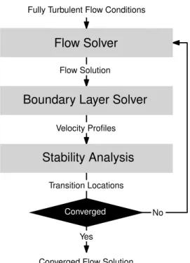
The main drawback to linear stability theory based transition modelling is the difficulty in coupling it with RANS-based flow solvers and optimisation frameworks. Menter et al. [54] proposed several conditions that transition modelling method should satisfy for easy integration with any RANS-based solver. These included the use of only local mathematical operations and the ability to predict transition locations for three-dimensional simulations. Both of these conditions are not met by the eN transition model. The eN model requires boundary layer velocity profiles at each chord-wise position, which are difficult for a RANS-based solver to obtain. This is because the edge of the boundary layer is difficult to deter-mine, many elements will make up a chord-wise boundary layer slice and grids may be split into different blocks for parallel computing [54]. TheeN model is also only able to model transition on an entire three-dimensional aircraft or wings by performing transition analysis on stacked two-dimensional slices.
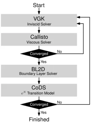
Coupling of theeN transition model with CFD codes is therefore somewhat complex and is outlined in figure 2.11. First, a flow solution with fully turbulent or laminar flow is obtained. A two dimensional streamline slice is then passed to a boundary layer solver which is used to generate velocity and pressure profiles along the chord-length. This is then passed to the stability analysis code which generates critical N-factor envelopes and locates a transition position. Transition is then prescribed at this location in the CFD flow solver and a new flow solution is obtained. The solution from this is again analysed and a transition location found. This process is repeated until the transition location converges to its final value. Given the complexity of effectively coupling stability based transition models with modern flow solvers, there has been a push for truly local transition modelling methods. This has lead to the development of transport equation models. These can be thought of as an ex-tension to empirical criteria. The general idea is to model transition using a flow property referred to as intermittencyγ that dictates the laminarity of the flow, whereγ = 0 is fully laminar andγ= 1 is fully turbulent. When applied to CFD, this term is used to scale eddy viscosity within the flow [54]. Intermittency is then related only to local flow properties, rather than local boundary layer properties such as used in empirical criteria.
Flow Solver
Boundary Layer Solver
Converged Stability Analysis Transition Locations Velocity Profiles Flow Solution No Yes
Fully Turbulent Flow Conditions
Converged Flow Solution
Figure 2.11:Workflow for CFD solver and linear stability theory transition model coupling.
The most popular transport equation based approach is the γ−Reθ model, developed by
Menter et al. [47, 55]. This is a two equation transition model for intermittency and transi-tional momentum thickness Reynolds number. Another transport equation based model has been developed by Coder and Maughmer [56]. This is based on the work of Drela and Giles [57] where amplification factor is related to local flow variables. Transport equation based approaches have seen a large amount of research over the past decade and are implemented in many commercial RANS-based CFD solvers. While the approach is maturing, physical modelling of flow stability has remained the preferred method used within the aerospace industry [15, 41].
2.3
Delaying Transition
The key to the design of NLF aerofoils and wings is the passive prevention of transition. Firstly, efforts must be made to ensure that transition follows the natural path, rather than via bypass or attachment line contamination. Once this is done, passive extension of laminar length is obtained via the tailoring of aerodynamic pressure gradient so as to dampen the growth of primary instabilities within the boundary layer.
The type of pressure gradient required depends on the instability types that dominate the flow transition process. TS instability waves are suppressed via the use of a favourable pres-sure gradient. This can be used to reduce instability amplification, remove inflection points from within the boundary layer, re-laminarise a turbulent boundary layer and reduce the size of turbulent spots [7, 45, 58, 59]. Favourable pressure gradient is, however, unsuitable
for flows dominated by crossflow instabilities, as this causes instability amplification espe-cially towards the leading edge. Instead, a strong leading edge pressure rise followed by a slight adverse pressure gradient is best [60].
These conflicting pressure gradient profiles are shown in figure 2.12. The type of insta-bility dominating the flow transition process is determined by the sweep angle Λ. Three sweep regimes can be defined: TS dominated whenΛ < 25◦, TS and CF dominated when
25◦ < Λ < 30◦and CF dominated when 35◦ > Λ[9]. Flows with transition dominated by TS instability waves are found on subsonic aircraft where no sweep angle is needed. For transonic aircraft such as modern commercial transport aircraft, sweep angles within the TS and CF dominated regime are used as this reduces the leading edge normal flow velocities and so wave drag. Sweep angles above 35◦are found on supersonic aircraft.
Cp
Tolmein-Schlichting Instability Crossflow Instability
x/c
Figure 2.12:Ideal pressure distributions for Tollmien-Schlichting and Crossflow instability suppression [60].
2.3.1 Design Considerations for NLF
While NLF is a promising drag reduction method, its practical implementation is difficult to achieve due to the numerous and often conflicting design requirements. For subsonic NLF design, a favourable pressure gradient can be used to suppress TS instability growth which is the only instability type present. This is done by changing aerofoil shape upstream and shifting the point of maximum thickness aft. However, this can produce large pitching moments and thus incur additional trim drag penalties. If too large, this can negate any benefits found from NLF [61]. A balance between NLF and overall performance is also needed as designs with highly delayed transition resemble the Stratford profile [62]. This has a long favourable pressure gradient rooftop and short pressure recovery region with very little skin friction, but experiences rapid separation and aggressive stall characteristics [63].
Transonic NLF design is complex as NLF and supercritical wing design considerations dif-fer. At transonic speeds, wing sweep is required to avoid the formation of strong shocks and so high wave drag. Sweep also helps to delay shock position, which can trigger up-stream transition. However, sweep also leads to strong CF instability amplification that can dominate the transition process and is harder to suppress with passive control methods. On highly swept wings, NLF is not possible for this reason.
Increased wing sweep can also lead to attachment line instability and propagation of at-tachment line contamination, depending on the flight Reynolds number and leading edge radius. A small leading edge radius helps to avoid attachment line instability and contami-nation and also reduces the region where leading edge CF growth can occur [9]. However, a large radius is preferred for supercritical aerofoil design so as to create flow pre-compression which reduces shock strength and so wave drag. This is obtained by an initial spike in pres-sure at the leading edge that reflects between the sonic line and aerofoil surface [5]. This ini-tial pressure spike also helps to reduce leading edge CF instability amplification but makes it difficult to obtain a favourable pressure gradient downstream so as to suppress TS insta-bility growth. Additionally, while a favourable pressure gradient is needed, it can lead to very large pressure recovery which at transonic speeds, results in the formation of a strong shock, reducing the effectiveness of the laminar flow extension [2].
2.3.2 Transition Location Robustness
A further limitation to the use of NLF is the high sensitivity of transition location to geo-metric shape, surface roughness and operating conditions. It is common for NLF aerofoils to be very susceptible to large reductions in laminar length due to leading edge contami-nation, icing and surface damage [64, 65] as well as steps between panels, rivet bumps and general irregularities in the roughness and machining quality of the aerodynamic surface [9, 18]. Significant contamination can divert the transition process from natural transition and cause secondary instabilities or bypass. Slight changes to surface roughness can cause larger initial disturbance amplitudes via increased receptivity. As such, flight tests of lami-nar flow designs require highly smoothed single-piece aerodynamic surfaces, avoiding pan-els and rivets typically used for aircraft manufacturing. As transition is strongly affected by free-stream turbulence and environmental noise, lab-based research is difficult to carry out. Usable transition location estimations are only obtainable using low noise wind tunnels. Additionally, without consideration for a wide range of operating conditions, NLF designs are often highly point-optimum with poor off-design performance. As transition is influ-enced by pressure gradient, changes in Mach number, Reynolds number or angle of attack can all result in significant movement of the transition location. This can result in a strong ’drag bucket’ shape on an aerofoil’s lift/drag polar such as those found with the NACA 6-series aerofoils, designed for extended NLF [66]. Alternatively it may lead to a low drag divergence Mach number such as found with the NLF0215F and NLF0414F [67].
It is also found that aerofoils designed for extended laminar flow often perform worse at fully turbulent conditions than those designed for fully turbulent flow [68]. As such, de-sign of early NLF aerofoils typically involved comparison of laminar and fully turbulent characteristics to ensure performance is maintained if laminarity is lost [65, 69, 70].
2.4
Summary
The complex requirements for effective implementation of NLF, and the high sensitivity of NLF designs to changes in shape and operating conditions, has limited its use on com-mercial transport aircraft. A key challenge of NLF design is balancing the design practices
needed for the extension of laminar flow, and the tradition design methods used for re-ducing form and wave drag [71]. To further complicate the NLF design process, it is also important that the benefits found with NLF are maintained away from the optimum oper-ating environment by considering both on and off-design conditions. These benefits also need to be made more robust to uncontrollable factors such as surface quality, design shape or environmental conditions.
As the design of NLF aerofoils and wings has complex constraints, requirements and trade-offs, it is seen as a suitable problem for aerodynamic optimisation. Uncertainty analysis and robust design are also useful tools in the development of robust NLF as NLF aerofoils and wings are often highly sensitive to properties affecting transition location. These topics and their application to NLF design are explored in the next chapter.
Approaches to Aerodynamic Design
3.1
Aerodynamic Shape Optimisation
In broad terms, optimisation can be described as the selection of some design variables that, coupled with state variables, maximizes or minimizes an objective function subject to con-straints [72]. When applied to aerodynamic shape optimisation, state variables are typically flight conditions specified in the flow solver. These include Mach number, Reynolds num-ber, freestream turbulent intensity or lift coefficient. Design variables come from the chosen parametrisation method and describe the aerodynamic shape being optimised [73, 74]. The objective function is then an aerodynamic property output from the flow solver. This can be drag coefficient (Cd), lift coefficient (Cl), endurance (ML/D) or some other performance parameter. Constraints are typically equalities or inequalities applied to geometric sizing or other aerodynamic properties not directly being considered during the optimisation process. There are two fundamental approaches to performing optimisation. These are one-shot, or direct solution of the optimisation problem, and iterative convergence towards an op-timized solution [72]. One-shot approaches involve analytically solving the optimisation problem to directly obtain design variable inputs for the optimum objective function value. This approach is preferable as an exact solution is found quickly with low computational requirements. In practice, however, it is often not possible to solve the optimisation prob-lem due to its complex nature, CFD-based probprob-lems being an example of this [72]. Iterative approaches must instead be used for these type of optimisation problems as an optimum design is found instead via a guided trail and error process. This involves taking an initial guess at optimum design variable values that are then used to evaluate the objective func-tion. New values are then selected using the chosen iterative approach and the objective function evaluate again with the hope improved its value. This process is repeated until no further improvements are possible and an optimal design is found.
The most important step in this process is the selection of new design variable values. Meth-ods proposed for this can be categorized into Gradient-based and Gradient-free approaches. Gradient-based approaches determine the direction of search by evaluating the objective function first derivative with respect to the design variables whereas gradient-free methods select new design variables through methods that avoid knowledge of the design space.
Each approach has its benefits and drawbacks. The choice of an optimisation algorithm can be affected by the complexity of the objectives, constraints and limits placed on the de-sign problems. As such, optimisation problems are often described as either single-objective or multi-objective. Furthermore, choosing between a gradient-based and gradient-free ap-proach is influenced by the scope of the optimisation problem being addressed. Design problems are categorised as single-point or multi-point depending on the number of dis-crete operating conditions considered.
3.1.1 Gradient-Based Optimisation
By using objective function derivatives, gradient-based optimisation algorithms are able to quickly traverse the design space while continuously improving the objective function value. As such, gradient-based methods are fast, efficient and widely used for aerospace optimisation problems [75]. For a gradient-based approach to be suitable for the design problem being addressed, it must be possible to obtain the first and second order derivatives of the objective function, and the design space must have low modality [76].
The first order derivative is required to guide the optimisation while the second order derivative is used to evaluate convergence. Derivatives can be found using either analyt-ical methods, automatic or algorithmic differentiation, complex-step approximation or via finite difference [75]. The modality of the design space dictates the ability of the optimisation algorithm to move towards a global optimum. Due to the gradient dictating search direc-tion, gradient-based approaches are excellent at finding the global optimum for uni-modal problems. They do, however, struggle when multiple modes are present. It may be possible to avoid this issue by restarting the optimisation several times with different design vari-able values, but escaping the local optima already found remains challenging [76]. As such, gradient-based optimisation is unlikely to find the global optimum case for a high number of modes [75].
This illustrates the potential dependence of gradient-based methods on initial design vari-able values and prior knowledge of the design space. Modality in CFD-based shaped op-timisation at fully turbulent conditions has been studied by a number of authors and is considered to be low. Analysis by Yu et al. [77] found that optimisation of a full wing has a close to uni-modal design space. When transition modelling is included, there is no clear consensus. Robitaille et al. [78] performed gradient-based aerofoil optimisation with free transition and found that a global optimum was not reached, suggesting a multi-modal de-sign space. Youngren [79] performed multi-point aerofoil optimisation with free transition and reported that the design space resembled a minefield with large spikes in gradient that cause huge changes in design and transition location.
3.1.2 Gradient-Free Optimisation
Gradient-free methods do not require objective function derivatives and so are typically easier to implement and avoid both requirements set out for gradient-based optimisation [80]. They are better suited to highly modal design problems as new design variables are selected discretely rather than by moving in a favourable direction through the design space. How new design variables are chosen depends on the specific gradient-free method in use.
![Figure 4.2: Schematic of the panel discretisation method used by XFOIL [140].](https://thumb-us.123doks.com/thumbv2/123dok_us/1876074.2773923/59.892.193.765.183.474/figure-schematic-panel-discretisation-method-used-xfoil.webp)