Robust Graph Mode Seeking by Graph Shift
Hairong Liu [email protected]
Shuicheng Yan [email protected]
Department of Electrical and Computer Engineering, National University of Singapore, Singapore
Abstract
In this paper, we study how to robustly com-pute the modes of a graph, namely the dense subgraphs, which characterize the underly-ing compact patterns and are thus useful for many applications. We first define the modes based on graph density function, then pro-pose the graph shift algorithm, which starts from each vertex and iteratively shifts to-wards the nearest mode of the graph along a certain trajectory. Both theoretic analysis and experiments show that graph shift algo-rithm is very efficient and robust, especially when there exist large amount of noises and outliers.
1. Introduction
Graph is an important representation approach, espe-cially for data which cannot be represented in vecto-rial form. Even for data with vectovecto-rial form, many algorithms are essentially founded on graph represen-tation, such as graph based image segmentation (Shi & Malik, 2000) and graph based data clustering (Ng et al., 2002).
A dense subgraph refers to a coherent subset of ver-tices in a graph and such cohesiveness is not easy to be disturbed by noises and outliers, thus the dense subgraphs can robustly indicate key patterns. For ex-ample, in World Wide Web, dense subgraphs might be communities or link spam; in telephone call graph, dense subgraphs might be groups of friends or families. In these situations, the graphs are usually very sparse in global, but have many dense subgraphs of differ-ent sizes, these dense subgraphs are the natural focal points for studying graph structure and extracting the underlying meaningful patterns.
Appearing inProceedings of the 27thInternational Confer-ence on Machine Learning, Haifa, Israel, 2010. Copyright 2010 by the author(s)/owner(s).
In computer science, the pursue of maximal cliques (cliques that cannot be enlarged) (Ouyang et al.,1997) is a fundamental problem and has been widely studied for decades. The Motzkin-Straus theorem (Motzkin & Straus,1983) has proven that solving maximal clique problem is equivalent to finding the maxima of a quadratic function, namely the graph density func-tion used in this work. Thus, the maximal cliques correspond to the modes of the graph and the maxi-mal clique problem is actually the mode seeking prob-lem on graph. The weighted counterpart of maximal clique, dominant set, also corresponds to the mode of the graph, and has ever been used for pairwise clus-tering (Pavan & Pelillo,2007).
In machine learning literature, the one-class clus-tering/classification problem (Gupta & Ghosh, 2005; Crammer et al., 2008), which finds a small and co-herent subset of points within a given data set, rises naturally in a wide range of applications, from finding gene-modules to extracting documents’ topics, where many data points are irrelevant to the task at hand, or in applications where only positive examples are avail-able. Such coherent subset of points forms dense sub-graphs, thus, one-class clustering/classification prob-lem is closely related to the mode seeking probprob-lem on graph.
Owing to the commonality of the dense subgraphs in many applications, many algorithms have been pro-posed (Pavan & Pelillo,2007;Ouyang et al.,1997) for computing such subgraphs. These algorithms are how-ever usually heuristic and can only find partial dense subgraphs, and at the same time, these algorithms are usually very demanding in both computational cost and memory requirement.
In this paper, we propose the graph shift algorithm, which can find all significant dense subgraphs, with low time and memory complexity. The graph shift al-gorithm is very similar with mean shift alal-gorithm (Co-maniciu & Meer, 2002), a well-known non-parametric feature space analysis technique. Both algorithms can start from any start point, shift along a certain
tra-jectory, finally reach the nearest mode. Thus they can be considered as evolutionary strategies that per-form multi-start global optimization; however, mean shift operates directly on the feature space, while our graph shift operates on the affinity graph. In many sit-uations, we can only obtain the affinity graphs, some even with no corresponding vectorial representation, thus, our method can be considered to be a comple-ment method of mean shift. The same as mean shift, graph shift can be used for robust model seeking and clustering analysis.
The main contributions of this work are two-fold. 1) We define the modes of a graph and analyze its prop-erty. Although the mode of a graph is widely used in many areas, it has not been well defined and sys-tematically analyzed. 2) We propose the graph shift algorithm, which can efficiently approach the nearest mode of a graph from any start point. This algorithm provides a robust tool for mode seeking and cluster analysis on graph.
The rest of the paper is organized as follows. We de-fine the modes of a graph and analyze its properties in Section 2, then we present the graph shift algo-rithm in Section 3. The experimental evaluation of our algorithm for robust mode seeking and clustering is performed in Section 4, and we conclude this work in Section 5.
2. Modes of Graph
In this section, we first define graph density, then de-fine the modes of a graph. Finally we analyze the properties of graph mode, which shall guide the in-ference of graph shift algorithm presented in the next section.
2.1. Notations of Graph
A graph G is represented as G = (V, E, w), where
V ={v1,· · ·, vn}is the vertex set,nis the number of vertices,E⊆V ×V is the edge set, andw:E→IR∗+ is the (nonnegative) weight function. Vertices in G
correspond to data points, edges represent neighbor-hood relationships, and edge-weight reflects similar-ity between a pair of linked vertices. As is custom-ary, we represent the graphGwith the corresponding weighted adjacency (or similarity) matrix, more specif-ically, an n×n symmetric matrix A = (aij), where
aij =w(vi, vj) if (vi, vj)∈E, and aij = 0 otherwise. Clearly, if there are no self-loops, all the diagonal ele-ments ofA are zeros. In this paper, we only consider graphs with no self-loops.
Let S ={1,· · ·, n} be the index set of the vertex set
V, for any subset T ⊆ S, a subgraph GT of G with
vertex setVT ={vi|i∈T}is introduced and the cor-responding edge set is ET ={(vi, vj)|(vi, vj)∈E, i∈
T, j∈T}.
2.2. Probabilistic Coordinate On Graph
The probabilistic coordinate on graphGis defined as a mapping X : V → ∆n, where ∆n = {x ∈ Rn :
x ≥ 0 and|x|1 = 1}, that is, the mapping from the vertex set V to the standard simplex of Rn. Each
point x ∈ ∆n represents a probabilistic combination
of vertices, called probabilistic cluster, and xi, the i
-th component of x, represents the probability of this probabilistic cluster contains vertex vi. Since under
the probabilistic coordinate, a pointxuniquely corre-sponds to a probabilistic cluster and vice versa, we will refer to them interchangeably. For a point x, xi = 0 means that this probabilistic cluster does not contain vertex vi. The indices of all nonzero components ofx
constitute its support, denoted as σ(x) = {i|xi 6= 0}, and it corresponds to a subgraphGσ(x). Particularly, the coordinate of the probabilistic cluster containing only vertex vi is Ii, whose i-th component is 1, and other components are 0.
Since aij represents the affinity value between vertex vi and vertex vj, the affinity value between point x
and pointy can be defined as follows:
a(x, y) =X
i,j
aijxiyj=xTAy (1)
Note thata(Ii, Ij) =aij, which is consistent with the definition for the weights of edges.
2.3. Graph Density and Modes
The affinity value between a point x and itself is
a(x, x) = xTAx, abbreviated by g(x). As a good
cluster should be the one in which strongly associated vertices should have edges with large affinity values connecting each other in the graph, g(x) is a natural measure of the cohesiveness (dense) of the probabilis-tic clusterx, which is referred to as graph density in this work.
We may reveal the meaning of the graph density from the graph constructed from a data set D = {di|i = 1,· · ·, n}in feature space, where vertexvicorresponds to data di,w(vi, vj) =K(di, dj), i6=j and w(vi, vi) = 0. K is a kernel function defined on feature space. The probabilistic coordinate x can be considered to be a distribution, namely the probability of choosing vertexvi(thus, datadi) isxi. Suppose we sample this
distribution N (N → ∞) times, then the number of data di is N xi. At point di, the density is f(di) =
P
jN xjK(di,dj)
N , then the average density of these N
points are: fav = P iN xif(di) N = X i,j xiK(di, dj)xj (2)
SinceK(x, x)≥K(x, y), the average density will reach maxima when these points are identical to one point
di, that is, when x= Ii, i∈ S. However, if we only consider the contribution of a point to other points, not considering the contribution of the point to itself, that is, we set K(x, x) = 0, then the average density of theseN points are:
fav =X
i6=j
xiK(di, dj)xj=xTAx=g(x) (3) whereAis the adjacency matrix of graphG. It means that the graph density is the limit of average density whenN → ∞and not considering self contribution. Note the differences between graph density and den-sity in feature space: graph denden-sity considers all mu-tual contribution within a probabilistic cluster, not considering self contribution and the contribution of points outside this probabilistic cluster; while the den-sity in feature space consider the contribution of all other points to one point. Owing to not considering the contribution of the points outside the probabilistic cluster, graph density is not sensitive to outlier; also because the graph density considers all mutual con-tribution within the probabilistic cluster, it is more robust to noises.
Definition 1. The modes of a graphGare local max-imizers of graph densityg(x) =xTAx.
For a pointx, the subgraph corresponds toxisGσ(x), composed by all vertices whose indices are inσ(x). If
x∗ is a local maximizer (mode) of g(x), then Gσ(x∗)
is a dense subgraph. Such dense subgraphs are very important in many applications. For example, 1) they are maximal cliques in graph analysis; 2) they repre-sent the core of a cluster in cluster analysis; and 3) they represent common patterns in common pattern detection problem.
2.4. Properties of Modes
Since the modes are local maximizers of g(x), to find these modes, we need to solve the standard quadratic optimization problem (StQPs) (Bomze,2002):
maximize g(x) =xTAx
subject to x∈∆n (4)
It is a constrained optimization problem, and a local maximizer x∗ ∈ ∆n must satisfy the
Karush-Kuhn-Figure 1.(a) Geometric explanation of graph mode. x∗is the mode of graphG, all the vertices (red points) belonging to Gσ(x∗) are on the sphere {y|a(x∗, y) = g(x∗)} and all
other vertices are within the space {y|a(x∗, y) ≤ g(x∗)}. (b) The relation between the mode of graph and the mode of its subgraph. x∗ is the mode of a subgraph, whether it is the mode of graphGdepends on whether there is no vertex (blue point) within the space{y|a(x∗, y)> g(x∗)}. For better viewing, please see color pdf.
Tucker (KKT) condition for problem (4), i.e., the first-order necessary conditions for local optimality. That is, there existn+ 1 real constants (Lagrange multipli-ers)µ1,· · ·, µn andλ, with µi≥0 for alli= 1,· · ·, n, such that:
(Ax∗)i−λ+µi= 0 (5)
for alli= 1,· · ·, n, andPn
i=1x ∗
iµi = 0.
Since both x∗i and µi are nonnegative for all i = 1,· · ·, n, the latter condition is equivalent to saying thati∈σ(x∗) impliesµi= 0. Hence, the KKT condi-tions can be rewritten as:
(Ax∗)i
=λ, i∈σ(x∗);
≤λ, i /∈σ(x∗). (6)
Note that (Ax∗)i = a(x∗, Ii), the affinity value
be-tween clusterx∗ and vertexi, thus (6) has an obvious geometric meaning, which is summarized in the follow-ing theorem.
Theorem 1. Ifx∗is the mode of graphG, then 1) the affinity values between x∗ and all the vertices in the subgraph Gσ(x) are identical to g(x∗); 2)the affinity values between x∗ and other vertices of graph G are not larger thang(x∗). At the same time, ifx∗satisfies 1) and 2), then it is the mode of graphG.
Proof: According to (6), x∗TAx∗ = P
ix∗i(Ax∗)i =
P
ix∗iλ=λ. Since KKT is a necessary condition, then
if x∗ is the mode, it must satisfies 1) and 2). At the same time, when equality constraints are affine func-tions, inequality constraints and the objective function are continuously differentiable invex functions, KKT
condition is also sufficient, thus ifx∗satisfy 1) and 2), it is the mode of graph G.
Theorem 1 tells that if x∗ is a mode of graph G, then all the vertices belonging to subgraph Gσ(x) are on the sphere {y|a(x∗, y) = g(x∗)}, and all the ver-tices not belonging to subgraphGσ(x)are in the space {y|a(x∗, y) ≤g(x∗)}. Figure 1(a) illustrate such sce-nario, x∗ is a mode, σ(x∗) = {v1, v2, v3, v4}, they all lie on the sphere{y|a(x∗, y) =g(x∗)}.
2.5. Modes of Subgraph
In many situations, graphGis very large, that is, it has many vertices and edges, it is very inefficient to deal with them as a whole. Note that σ(x∗), the support of the modex∗, usually contains very limited number of vertices and ˜x∗ = {x∗i|x∗i > 0}, which retains all nonzero components of x∗, is also the mode of the subgraphGσ(x∗). SubgraphGσ(x∗)contains onlym=
|σ(x∗)| vertices, thus much easier to deal with. This phenomenon inspires us to search for the modes ofG
through the modes of its subgraphs.
For a subgraph GT, suppose one of its mode is x∗T, according to Theorem 1. (Ax∗T)i =λ, i∈σ(x∗T); ≤λ, i /∈σ(x∗T). (7) whereσ(x∗T)⊆T ⊆S.
By adding zeros to the components whose index are in the set S−T, we can expand the m dimensional vectorx∗T tondimensional vectorx∗. The problem is whetherx∗is also the mode of graphG. The following theorem answers this question.
Theorem 2. A mode x∗
T of the subgraphGT is also
the mode of graph G if and only if for all vertex vi, a(x∗, Ii) ≤ g(x∗) = gT(x∗T), i ∈ S−T, where x
∗ is obtained from x∗T by adding zeros to the components whose indices are in the setS−T.
Proof: Sincex∗ is obtained fromx∗T by adding zeros to the components whose indices are in the setS−T, thenσ(x∗) =σ(x∗T),g(x∗) =gT(x∗T), and (Ax∗)i =λ, i∈σ(x∗); ≤λ, i∈T, i /∈σ(x∗); =a(x∗, Ii), i∈S−T. (8) whereλ=g(x∗) =g(x∗T). If a(x∗, I
i) ≤ g(x∗) = λfor all i ∈ S−T, according
to Theorem 1, x∗ is also the mode of graph G. If
a(x∗, Ii)> g(x∗) =λfor somei∈S−T, thenx∗does
not satisfy the KKT condition, according to Theorem 1, thus it is not the mode of graph G.
Theorem 2 has an intuitional geometric meaning: Since the affinity values between a mode x∗ of graph
G and the vertices in subgraph Gσ(x∗) are
identi-cal to a constant value λ, we can regard the sphere {y|a(x∗, y) =λ}to be a separating surface, if no newly added points fall into the space{y|a(x∗, y)> λ}, then
x∗is still the mode of the expanded graph; otherwise,
x∗ is not a mode of the expanded graph. Figure 1(b) illustrates this point, if the newly added point is vi, thenx∗is still the mode of the expanded graph; how-ever, if the newly added point isvj,x∗is not the mode
of the expanded graph.
3. Graph Shift Algorithm
There are many algorithms to obtain a local maxima of StQP (4), from any initializationx(0). In this section, we first review the most popular method, replicator dynamics (Weibull, 1997). Then we will present the neighborhood expansion procedure, which can expand the support of the mode of a subgraph to its neighbor-hood. The combination of these two steps forms our graph shift algorithm.
3.1. Mode Seeking by Replicator Dynamics
Replicator dynamics, which arises in evolutionary game theory, is the most popular method to find the local maxima of StQP (4). Given an initialization
x(0), corresponding local solutionx∗ of StQP (4) can be efficiently computed by the discrete-time version of first-order replicator equation, which has the following form:
xi(t+ 1) =xi(t)
(Ax(t))i
x(t)TAx(t), i= 1,· · ·, n. (9)
It can be observed that the simplex ∆n is invariant
under these dynamics, which means that every tra-jectory starting in ∆n will remain in ∆n. Moreover,
it has been proven in (Weibull, 1997) that, when A
is symmetric and with nonnegative entries, the objec-tive functiong(x) =xTAxstrictly increases along any
nonconstant trajectory of (9), and its asymptotically stable points are in one-to-one correspondence with strict local solutions of StQP (4).
Note that Equation (9) has a property: if xi(t) = 0, then xi(t+ 1) = 0 andxi(t) does not affect the com-putation of xj(t), j6=i, which means that during the evolution procedure, replicator equation (9) can drop vertices, but it cannot automatically expand the ver-tices. Thus, from a subgraphGT, it can find the mode
ofGT, but this mode may not be the mode of graphG.
In the following subsection, we will present the method of expanding vertices from the modes of subgraphs.
3.2. Neighborhood Expansion from Modes of Subgraphs
From a mode x∗T of the subgraph GT, according to Theorem 2, we can judge whether it is also the mode of graphG. If yes, then no further step is required; if not, we need to find an update vector ∆x,g(x∗+∆x)> g(x∗), where x∗ is obtained from x∗T by adding zeros to the components whose indices are in the setS−T. Sincex∗is not a mode ofg(x), according to Theorem 2, there are some verticesvi,a(x∗, Ii)> g(x∗),i∈S−T. We define a vectorv with
vi= 0, i∈σ(x∗) max(a(x∗, Ii)−g(x∗),0), i /∈σ(x∗) . (10) Suppose s=P ivi, ζ = P ivi2 and ω = P i,jviaijvj,
then s > 0 and ζ > 0. We update x∗ in direction
b=
−x∗is, i∈σ(x∗)
vi, i /∈σ(x∗) . That is, decreases the pos-sibility of vertices belonging to current mode and in-creases the possibility of vertices with large rewards. Supposeg(x∗) = ˜λ, then (Ax∗)i= ˜λ, i∈σ(x∗), g(x∗+tb)−g(x∗) = 2t(1−ts)(ζ+ ˜λs)−ts(2−ts)˜λ+ωt2 = −(˜λs2+ 2sζ−ω)t2+ 2ζt (11) According to x∗i ≥0, i∈ σ(x∗), x∗i −tx∗is≥0, then t≤1 s. When ˜λs
2+2sζ−ω≤0, the increase fromg(x∗) to g(x∗+tb) will reach maximum at t∗ = 1s; When ˜
λs2+ 2sζ−ω >0, the increase fromg(x∗) tog(x∗+tb) will reach maximum at t∗ = min{1
s, ζ
˜
λs2+2sζ−ω}, and
the update vector is:
∆x=t∗b, (12)
which is calledneighborhood expansion vector. The update fromx∗ to x∗+tbnot only increases the value of g(x), but also expands the support σ(x∗) to its neighborhood, which is the desirable property. 3.3. Graph Shift Procedure
The replicator dynamics and the neighborhood ex-pansion procedure have complementary properties: 1) replicator dynamics can efficiently drop vertices, but neighborhood expansion cannot; 2) neighborhood ex-pansion can expand the support, but replicator dy-namics cannot. Their combination leads to the graph shift algorithm, which is summarized in Algorithm 1. Algorithm 1 is an EM-style procedure, the neighbor-hood expansion procedure expands current subgraph
Algorithm 1Graph Shift Algorithm
Input: The affinity matrixAof graph G, the start pointx(a vertex, or a cluster of vertices)
repeat
Evolvextowards the mode of subgraphGσ(x)by replicator dynamics (9)
if x is not the mode of graphGthen
Updatexby neighborhood expansion vector end if
untilxis the mode of graph G
to its neighborhood, thus provides a much larger lower bound ofg(x), which corresponds to the mode of cur-rent subgraph; while replicator dynamics procedure evolves towards this lower bound, and guarantees to reach this lower bound. These two steps iterate un-til a local maxima is reached. In the neighborhood expansion procedure, only nearest vertices are added into current subgraph, and in the replicator dynamics procedure, most of vertices are dropped, and only a very compact cluster of vertices are retained. Thus, our graph shift algorithm always operates on small subgraphs, which is very efficient, both in time and memory.
The main computation load is the replicator dynamics procedure, which evolves toward the mode of current subgraph. Suppose the average number of edges in the subgraph ish, and the average number of iterations for the replicator equation is t, then the time complexity of the replicator dynamics procedure isO(th), and the space complexity is O(h). The total time complex-ity of graph shift procedure is thenO(lth), where l is the number of iterations for the shrink and expansion phases.
4. Experiments
We evaluate the proposed graph shift algorithm on two tasks: mode seeking and cluster analysis. Since under real-world scenarios, the graph usually contains considerable noises and outliers, in our experiments, we mainly focus on these scenarios.
4.1. Detecting Common Pattern as Mode Seeking on Graph
A pattern is a set of feature points with fixed relative spatial relation. Two instances of a common pattern not only need to be similar in corresponding feature points, but also need to have similar spatial layout. The common pattern problem is: given two sets of fea-ture points, are there any common patterns between them and where they are? We will show that this
problem is identical to mode seeking on a graph with large amount of noises and outliers. Thus, the com-mon pattern problem is a good test-bed to evaluate the effectiveness and robustness of our graph shift al-gorithm.
Suppose two sets of feature points are P andQ, with
nP and nQ feature points, respectively. Each fea-ture point contains local feafea-tures and coordinates. For each point pin P, according to the local features, we may find some similar pointsq in Q. Each such pair (p, q) is a possible correspondence and all such pairs form the correspondence set C = {(p, q)|p ∈ P, q ∈
Q, pandqhave similar local features}.
We construct a graph G based on C with each ver-tex of G representing a correspondence in C. Edge
e= (vi, vj) connects vertexvi andvj, and reflects the relation between correspondences ci and cj. For two correspondencesci= (pi, qi) andcj= (pj, qj), suppose the distance betweenpi andpj in the first image, and the distance betweenqiandqjin the second image, are
lpipj andlqiqj, respectively. Obviously, to align these two correspondences, we need to scale the second im-age by a factor oflpipj/lqiqj.
Suppose the correct scale factor of a common pattern iss, we can definewij, the weight of edgee= (vi, vj),
as follows:
wij= exp(−|lpipj−slqiqj| 2
ς2 ) (13)
Obviously, under such definition, common patterns correspond to dense subgraphs in G, which is illus-trated in Figure 2. The common pattern correspond-ing to the modex∗can be recovered from the vertices of subgraph Gσ(x∗), with every vertex corresponding
to a correct correspondence.
Graph G has two characteristics: 1) There are large amount of vertices and most of them represents incor-rect correspondences. The number of vertices is nearly
nPnQ, but only m correct correspondence, where m
is the number of points in common pattern. 2) Many edges have large weights. Since the weight only reflects scale relation of two correspondences, many edges, such as the edges between incorrect correspondences, may accidently have large weights. The number of such edges is usually several order of magnitude than the number of edges between correct correspondences. These two characteristics pose a great challenge on mode seeking.
We first conduct an experiment on point sets and com-pare our method with spectral method in (Leordeanu & Hebert, 2005), which is the state-of-art method to
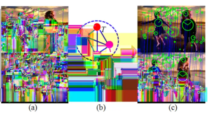
Figure 2.Common pattern detection corresponds to mode seeking on graph G. Find all candidate correspondences shown in (a) by local features (for clarity, only a small subset of the candidate correspondences are shown), and then construct the graphGin (b). The common pattern corresponds to the dense subgraph (mode)T ofG.
Figure 3.Performance curves for our method vs. the spec-tral method in (Leordeanu & Hebert, 2005). The mean performance (number of correct matches) is shown as a solid red line (our method) and a solid blue line (spectral method), Onestd below the mean is shown as red dotted lines for our method and blue dotted lines for the spectral method. Left figure: no Gaussian noise (η = 0). Right figure: added Gaussian noise (η= 4).
find correct correspondences. We generate a point set
T withnT points, add Gaussian noiseN(0, η) and
ro-tate it to obtain two version ofT. We then add outliers to them by randomly selecting points in the same re-gion and obtain the two point setP andQ. Since the points themselves are not distinctive, the number of vertices isnPnQ. We fix the number of points in the common pattern, nT = 15, and vary the number of outliers. Both algorithms ran on the same data sets over 30 trials and both the mean performance curves and the curves of one standard deviation below the mean are plotted. We score the performances of these two methods by counting how many correspondences agree with the ground truths.
The result is shown in Figure 3. Obviously, the spec-tral method is sensitive to outliers and its performance curve drops fast; however, our proposed graph shift method works remarkably well. This is because the
Figure 4.Comparison of cumulative accuracy of near-duplicate image retrieval on Columbia database.
eigenvectors are affected by all weights, especially all the large weights, no matter they are correct or not; however, our graph shift method just try to find a subgraph with all edges have high weights and such weights are usually correct.
We also conduct an experiment on near-duplicate image retrieval, which plays an important role in many multimedia applications. Near-duplicate images usually have a large common pattern, thus judging whether two images are near-duplicate or not is also a mode seeking problem on graph. The experiment is conducted on the Columbia database, which con-tains 150 near-duplicate pairs and 300 non-duplicate images (600 images in total). For fair comparison, we first rank all images using global features as done in (Zhu et al., 2008), then re-rank the images in top 50 based on the size of detected common patterns. We use SIFT features to find all possible point correspon-dences and the weightwij is computed by (13). Since just at correct scale, common patterns correspond to the mode of graph, we search for 11 scales. In Fig-ure 4, the retrieval performance is plotted and com-pared with the state-of-art method, called NIM (Zhu et al., 2008), which finds common patterns by non-rigid mapping. Obviously, our method gets better cu-mulative accuracies (ratio between correctly retrieved images in top N images and total number of query images), which verifies that our method can correctly find the modes of the graph.
4.2. Cluster Analysis
Graph shift procedure is a natural clustering tool, and all the vertices shift toward the same mode should be-long to a cluster. According to the need, there are two variants of clustering methods based on graph shift: 1) The number of clusters is unknown. In this case, we regard each mode with large density as the core of a cluster, and all the vertices shift towards this mode
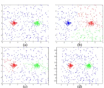
Figure 5.Clustering on data with uniform distributed background points. (a) the data set, (b) clustering result of k-means, (c) clustering result of spectral clustering, (d) clustering result of our method. For better viewing, please see original color pdf.
belong to this cluster, other vertices can be assigned to one cluster according to affinity value or left un-grouped. 2) The number of clusters K is specified. In this case, we just selectK modes with the largest densities, and then assign other vertices to these K
clusters.
We first consider the problem of extracting dense clus-ters from cluttered background. Many real world prob-lems belong to this kind, such as image segmentation and perceptual grouping. Because many points should not belong to any clusters, such as the background of an image, the partition methods, such as k-means and spectral clustering method, are not expected to work well, due to their insisting on partitioning all the in-put data into coherent groups. Our method, on the contrary, appears to be particularly suited for such applications, since it allows one to extract as many clusters as desired, while leaving the remaining points (namely, the clutter) un-grouped.
To illustrate this point, consider the toy data set shown in Figure 5(a), which contains two dense clusters of Gaussian random points surrounded by uniformly dis-tributed clutter points. For comparison, we choose k-means and spectral clustering, two representative par-tition methods, based on vectorial representation and affinity data, respectively. The clustering results of k-means, spectral clustering and our method are illus-trated in (b),(c),(d), respectively. As expected, both k-means and spectral clustering cannot work well; while our method can automatically uncover the two dense clusters and separate them from the background.
Table 1.Clustering results and computational cost for spectral clustering (SC), affinity propagation (AP) and our method on the shape matching affinity data.
SC AP Our Method
Clusters 70 64 70
Precision 73% 76.5% 85.36%
NMI 88.63% 88.27% 91.41%
Time(seconds) 11.6904 514.9922 1.2320
We also conduct an experiment on the affinity data from shape matching. The database is MPEG-7 shape database, there are 70 categories and each category contains 20 shapes. For each two shapes, we calcu-late their matching score (affinity value) using certain shape matching method, thus obtain a 1400×1400 affinity matrix. Such affinity data has no correspond-ing vectorial representation; at the same time, it usu-ally contains a large amount of noises, since for dif-ferent pairs of shapes, their matching scores are com-puted independently, and the matching method may produce wrong results on some pairs of shapes. We compare our method with the spectral clustering and affinity propagation (Frey & Dueck, 2007), both of which are classical methods based on affinity matrix. The result is shown in Table 1. The performance of clustering is measured by both the precision and normalized mutual information (NMI). Both spectral clustering and our method can specify the number of clusters, but affinity propagation can only approxi-mate the specified number. Obviously, our method outperforms spectral clustering and affinity propaga-tion, and a possible explanation is that the affinity ma-trix contains many noises and our method is inherently noise-resistent. At the same time, our method spends much less time. Note that AP needs to search an ap-propriate preference value, thus it runs the clustering algorithm many times and spends very long time.
5. Conclusions and Future Work
In this paper, we define the mode of a graph, which corresponds to a coherent subset of vertices, thus is in-herently robust to noises and outliers. We propose the graph shift algorithm to robustly compute all modes. The experimental results show that our algorithm is surprisingly robust to noise and outliers. Future works include more efficient methods on large scale data and applications in one-class clustering/classification prob-lems.
6. Acknowledgement
This work is supported by National Research Foun-dation/Interactive Digital Media Program, under
re-search Grant NRF2008IDMIDM004-029, Singapore.
References
Bomze, M. Branch-and-bound approaches to standard quadratic optimization problems. Journal of Global Optimization, 22:17–37, 2002.
Comaniciu, D. and Meer, P. Mean shift: A robust ap-proach toward feature space analysis. IEEE Trans-actions on Pattern Analysis and Machine Intelli-gence, pp. 603–619, 2002.
Crammer, K., Talukdar, P., and Pereira, F. A rate-distortion one-class model and its applications to clustering. In Proceedings of the 25th Interna-tional Conference on Machine Learning, pp. 112– 119, 2008.
Frey, J. and Dueck, D. Clustering by passing messages between data points. Science, 315:972–974, 2007. Gupta, G. and Ghosh, J. Robust one-class clustering
using hybrid global and local search. InProceedings of the 22nd International Conference on Machine Learning, pp. 273–280, 2005.
Leordeanu, M. and Hebert, M. A spectral technique for correspondence problems using pairwise con-straints. In Proceedings of the International Con-ference on Computer Vision, pp. 1482–1489, 2005. Motzkin, T. and Straus, G. Maxima for graphs and
a new proof of a theorem of Turan. Theodore S. Motzkin: selected papers, pp. 311–314, 1983. Ng, Y., Jordan, I., and Weiss, Y. On spectral
clus-tering: analysis and an algorithm. In Advances in Neural Information Processing Systems, volume 2, pp. 849–856, 2002.
Ouyang, Q., Kaplan, D., Liu, S., and Libchaber, A. DNA solution of the maximal clique problem. Sci-ence, 278:446–448, 1997.
Pavan, M. and Pelillo, M. Dominant sets and pairwise clustering. IEEE Transactions on Pattern Analysis and Machine Intelligence, 29:167–172, 2007. Shi, J. and Malik, J. Normalized cuts and image
seg-mentation. IEEE Transactions on Pattern Analysis and Machine Intelligence, 22:888–905, 2000. Weibull, W. Evolutionary game theory. The MIT
press, 1997.
Zhu, J., Hoi, H., Lyu, R., and Yan, S. Near-duplicate keyframe retrieval by nonrigid image matching.