Marginal tax rates and income inequality: a quantitative-theoretic analysis

Working Paper 9508

MARGINAL TAX RATES AND INCOME INEQUALITY: A QUANTITATIVE-THEORETIC ANALYSIS

by David Altig and Charles T. Carlstrom

David Altig is an assistant vice president and economist and Charles T. Carlstrom is an economist at the Federal Reserve Bank of Cleveland. For helpful comments, the authors thank Ben Craig and seminar participants at

Arizona State University, Bowling Green State University, and the April 1995 meeting of the Federal Reserve System Committee on Macroeconomics.

Working papers of the Federal Reserve Bank of Cleveland are preliminary materials circulated to stimulate discussion and critical comment. The views stated herein are those of the authors and not necessarily those of the Federal Reserve Bank of Cleveland or of the Board of Governors of the Federal Reserve System.

Abstract

In this paper, we employ a quantified general equilibrium model to study the effects of changes in marginal income-tax rate structures on the distribution of income. Our approach builds on recent efforts by Fullerton and Rogers (1 993) in extending the well-known work of Auerbach and Kotlikoff (1987) to allow for many different cohort types, and hence a nontrivial endogenous distribution of income. In addition, we utilize (and describe) a solution algorithm that allows us to study the distributional consequences of distortions on labor and consumption arising from actual discrete rate structures taken from the U.S. tax code.

Focusing on variations of the 1965, 1977, 1984, and 1989 U.S. rate schedules, our main conclusions are as follows:

1. The distortionary effects of marginal rate structures on individual saving and labor-supply decisions may explain significant elements of recent trends in income inequality. For example, the model predicts a change in the Gini index of inequality between 1984 and 1989 that is almost half of the change that actually occurred.

2. "Static" revenue calculations

--

those assuming no change in behavior following marginal rate changes

--

substantially overstate the long-run revenue effects of shifting from our alternatives to the 1989 tax structure. For example, under static assumptions, replacing the 1977 tax code with that from 1989 causes steady-state revenue to fall.

However, the full general-equilibrium impact causes long-run revenues to increase slightly. 3. Compared to the 1977 and 1984 tax structures, a shift to the 1989 code yields steady-state welfare gains that are strongly concentrated among individuals at the upper tail of the lifetime income distribution. Furthermore, for these cases, a rising tide does not raise all boats: Those at the lower end of the lifetime income distribution have higher utility in steady states under the alternatives, even though long-run aggregate income is higher under the 1989 regime.

1. Introduction

Change is the constant of U.S. tax policy. Since the early 1960s, the federal personal income tax code has undergone three major reforms and numerous minor

revisions. All of the major legislative changes

--

passed into law in 1964, 198 1, and 1986

--

involved, among other things, substantial alterations in the structure of marginal tax rates.' Economists, trained to believe that prices and incentives affect human behavior, are inclined to accept the theoretical proposition that these changes matter. But how much they matter is an item of considerably more dispute, and most agree that the issue is ultimately empirical.

Much of the current interest in tax rate structures has focused on the related issues of income distribution and revenue generation, with the empirical arms of this research broadly embracing the contribution of tax changes to trends in income inequality and the search for quantitative estimates of so-called Laffer curve relationships. In this vein, Feenberg and Poterba (1 993), Feldstein (1 993), Lindsey (1 990, 1993), and Slemrod (1993) all provide research that directly attacks these questions in light of recent tax reforms. From these studies, a consistent picture emerges of "a very substantial response of taxable income to changes in marginal tax rates" (Feldstein [1993, page 21). This observation is particularly strong for high-income taxpayers, who have been confronted with larger changes in tax rates than most of the general population, and have greater opportunities for adjusting to them.

Most of the conclusions in these studies are reached by examining or extrapolating from publicly available tax-return data. In this paper, we pursue a complementary

empirical strategy by building on the computable general equilibrium framework pioneered by Auerbach and Kotlikoff (1987). In particular, we adopt their basic simulation

approach, with two key extensions: First, we follow the recent work of Fullerton and

An excellent overview of these changes is provided in Pechman (1987).

Rogers (1993) and allow for many types of life-cycle agents, each distinguished by its labor efficiency endowments, and hence lifetime wealth. Second, we use a simple algorithm for solving Auerbach-Kotlikoff models with discrete tax codes. This second innovation allows us to examine marginal tax rate structures in their literal form.

Our basic approach is as follows: We take 1989 as a benchmark and calibrate the model so that, given the 1989 rate structure and plausible intertemporal elasticities of substitution in labor and consumption, the steady-state values we obtain from our

simulations match both the usual aggregate variables (the capital-output ratio, the risk-free interest rate, average tax rates, and so on) and the distributional characteristics (such as the Gini coefficient) implied by 1989 tax-return data. Based on the resulting quantitative framework, we examine the effects of different historical rate structures on the distribution of income.

Several characteristics of these experiments help to complete the pictures drawn by earlier studies. First, conditional on the model's structure and parameterization, our simulation approach provides a clear sense of private.labor-supply and saving responses to changes in marginal rate schedules. Because we abstract from exogenous variations in all other variables (including macroeconomic fluctuations, household characteristics, and net tax payments), all changes in the pre-tax distribution of income are due to the

distortionary effects of the different tax codes we consider. Furthermore, these effects are not confounded with changes in tax rules that are distinct from changes in rate structure per se.2

Second, for most taxpayers, tax reform alters the entire life-cycle path of marginal tax rates. This feature of tax policy can be, at best, only partially examined in existing microdata sets. Consider, for example, the analysis reported by Feldstein (1993), which

-

Our experiments do allow for some variation in basic exemptions and deductions. We note here that, in their studies, Feldstein and Lindsey also attempt to isolate the effects of rate changes from other changes in tax policy.

uses a panel of actual individual income-tax returns in tax years 1985 and 1988.

Feldstein's approach involves grouping taxpayers according to the marginal tax rates they faced in 1985, and comparing the percent changes in income from 1985 to 1988 with percent changes in marginal net-of-tax rates (1 minus the tax rate) over the two years.3

A specific example clarifies the potential contribution of the life-cycle simulations we conduct. In our work, the simulation comparable to the natural experiment examined by Feldstein contemplates a shift from the 1984 to 1989 rate structures, which are, respectively, nearly identical to the 1985 and 1989 codes. As with Feldstein's 1985 to

1988 comparison, most taxpayers in the 22 percent rate bracket in 1984 would face a 15 percent marginal rate in 1989: At the third year of the transition from the 1984 to 1989 tax code, approximately 17 percent of taxpayers in our model economy would experience a decline in the marginal rate from 22 percent to 15 percent, representing an increase of about 9 percent in the net-of-tax rate.4

However, this figure is not generally representative of net-of-tax rates for these taxpayers over the remainder of their life cycle. Furthermore, the average lifetime change in marginal rates for households in this group varies substantially, ranging from an average change in the life-cycle net-of-tax rate of about 8 percent to a scant 0.1 percent. The framework we employ is expressly designed to account for such life-cycle variations in tax rates, which, as this example indicates, can be quantitatively important.

Specifically, across the two years, Feldstein calculates the percent change in marginal tax rates and the percent change in various measures of income for three groupings of taxpayers: Those facing "medium" marginal tax rates in 1985 (22 percent to 38 percent), those facing "high" rates (42 percent to 45 percent), and those facing "very high" rates (49 percent and 50 percent). Elasticities are calculated as the ratio of differences in percent income changes across the rate groupings relative to the differences in percent rate changes. This general methodology was coined the "differences of differences" approach by Lindsey (1987).

Roughly 23 percent of taxpayers in Feldstein's 1985 sample fall into the 22 percent rate bracket. However, unlike our calculations, his sample excludes joint filers in rate brackets below 22 percent.

The final advantage of our approach is that, because all outcomes are the result of the explicit utility-maximizing decisions of taxpayers, the welfare consequences of tax- induced distributional effects can be directly assessed.

In each of our experiments, we examine U.S. marginal tax rate structures from 1965, 1977, and 1984 that have been adjusted for price and real output growth, and compare equilibrium outcomes under each to those from the (benchmark) 1989 code. To preview our results, we conclude that:

1. The distortionary effects of marginal rate structures on individual saving and labor- supply decisions may explain significant elements of recent trends in income inequality. For example, the model predicts a change in the Gini index of inequality between 1984 and 1989 that is almost half of the change that actually occurred. Furthermore, the tax code changes we simulate generate distributional effects that are broadly similar to the changes observed in the U. S. economy across the four years 1965, 1977, 1984, and

1989. For example, across these four years, the model generates patterns in the Gini coefficient and in the share of income received by the top 5 percent of income earners that are similar to those found in the data.

2. "Static" revenue calculations

--

those assuming no change in behavior following marginal rate changes

--

substantially overstate the long-run revenue effects of shifting from our alternatives to the 1989 tax structure. For example, under static

assumptions, replacing the 1977 tax code with that from 1989 causes steady-state revenue to fall. However, the full general-equilibrium impact causes long-run revenues to increase slightly.

3. Compared to the 1977 and 1984 tax structures, a shift to the 1989 code yields steady- state welfare gains that are strongly concentrated among individuals at the upper tail of the lifetime income distribution. Furthermore, for these cases, a rising tide does not raise all boats: Agents at the lower end of the lifetime income distribution have higher utility in steady states under the alternatives, even though long-run aggregate income is

higher under the 1989 regime. However, the welfare differences across the different rate regimes are very small for both lower- and middle-income taxpayers, and in many cases are dominated by general equilibrium effects on wages and interest rates.

In the next section, we lay out the basic structure of our framework. In section 3, we describe our calibration exercise, emphasizing the distributional aspects of the

quantified model. The balance of the paper is devoted to presenting the results summarized above.

2. The Model Economy A. Households and Preferences

Our model economy is populated by sequences of distinct cohorts that are distinguished by date of birth and lifetime labor productivity endowments. Each

generation born at a specific date contains 13 separate agent types, indexed by j, each with different exogenous labor efficiency profiles. With the exception of size, successive generations ofj-type agents are identical. All agents live 60 periods with perfect certainty, and each j-type cohort is l+n times larger than its predecessor.

Agents "born" at calendar date b choose perfect-foresight consumption (c) and leisure (I) paths to maximize a time-separable utility hnction of the form

where ui > 0 , uii < 0 , lim i+m ui = 0, limi+, ui = oo, and ui is the partial derivative of the

hnction u(.) with respect to argument i. The form of the utility function and the

subjective time-discount factor

p

are assumed to be the same for all agents. We require that P>O, but need not impose the condition that P<1.

Letting a:, be capital holdings for type j, age t agents at time s = b+t-1,

maximization of equation (1) is subject to a sequence of budget constraints given, at each time s, by

where r, is the real return to capital held from time s-1 to s, and z:, refers to lump-sum transfers from the government. We assume that aggregate wage payments at each time s,

w,, are distributed according to the efficiency levels of individual labor units. Furthermore, we assume that an individual worker's labor efficiency level is solely determined by his age and the lifetime income cohort of which he is a member. Thus, we denote the efficiency level of an age t member of cohort j by E: , wj, = E:w,.

The function T@,) is identical for all taxpayers and depends on taxable income, defined generally as

jjls

= yh - d(y{,), where y h = rsaj_l,s-I

+

w:, (1 - l;,), and the hnction d(.) specifies deductions and exemptions as a function of gross income.

Throughout, we will assume that d(.) is a linear function with a strictly positive first . '

deri~ative.~ We do not require that the function T(.) be everywhere continuous and differentiable. In fact, our analysis is conducted using U. S. personal income-tax codes that have the familiar discrete step-function structures.

B. Firnts and Technology

Output in the model economy is produced by identical competitive firms that combine capital and labor using a neoclassical, constant-returns-to-scale production technology. Letting yJ be the fraction ofj-type agents in each generation, aggregate capital (K) and labor (L) supplies (in per capita terms) are obtained from individual supplies as

Although this assumption is not necessary, it provides a reasonable description of historical income-tax structures in the United States in that simple linear regressions of deductions plus exemptions on income fit the data with a high R ~ .

and

13 60

where n is the constant rate of population growth. Note that, for simplicity, we have normalized the population so that the total number of age-60 agents is one, for all s.

The aggregate per capita production technology is written in terms of the capital- labor ratio, K, as

where qs is per capita output and f ( a ) is defined such that

f'

> 0 , f" < 0, lim

,

,

,

f'

= 0 , and lim

,,,

f'

= oo . The competitive wage and interest rates are given by

w, = q s -

K f ' ( 9

( 6 )

and

rs =

f

)s(' -

6 ,

where Sis the depreciation rate of physical capital.

C. The Government

Our interest in this paper is solely in the distortionary effects of different income- tax structures. Consequently, the government in our model has a very simple role: It raises revenue from income taxes, which it then rebates in the form of lump-sum payments to the individuals from whom taxes are collected. Thus, the government's activities in each period s are hlly captured by the "rule"

for all t, s, and j. Therefore, our simulations correspond to compensated demand

experiments, and effects from government policy arise only from the distortionary impact of the income-tax system.

3. Model Calibration

Our model is calibrated to Internal Revenue Service Statistics of Income data for the taxable returns of married persons filing jointly in 1989. In what follows, all references to income, taxpayers, and so on, should be understood as applying to this population.

Most of our choices for parameterizing the model are standard. Exceptions

involve the special features of our framework, specifically, the tax codes and the 13-agent- type structure. We therefore turn first to a discussion of how we quantifi these elements, followed by a discussion of the more familiar choices for preference and technology parameters. This section concludes with an overview of the equilibrium outcomes generated by our benchmark parameterization.

A. Labor EfJiciency ProJiles

The exogenous labor efficiency profiles in equations (2) and (4) are based on estimates provided by Fullerton and Rogers (1993), who use data from the Michigan Panel Study of Income Dynamics (PSID) to calculate life-cycle labor endowments.6 Using the notation developed above, and assuming that life begins in adulthood at age 20, these estimates imply that the labor efficiency endowments of a type j, age t agent are of the form

<'

= ebo+b,t+b2t2+b3t3

-

Focusing on a subsample that includes only households with stable marital histories over the 1970-1987 period, Fullerton and Rogers first fit a common wage function across all individuals. Specifically, they regress the log of average hourly earnings for each individual on a cubic in age and the interaction age and age-squared with sex, education, and race. The coefficients thus estimated are used to construct synthetic individual wage observations outside the 18-year period covered by the sample, as well as missing observations within the sample, which are then combined with actual wage observations to calculate lifetime incomes for all households. Finally, individuals are classified by lifetime income level into one of 12 groups, and separate wage profiles are estimated for each of the groups.

Values for the b coefficients for j-type groups 1 through 12, numbered in ascending order of lifetime income, can be found in tables 4-1 1 of Fullerton and Rogers.

Unfortunately, when we calibrate so that mean income from the model matches mean income in the Fullerton-Rogers data, the income levels implied by the 12-group disaggregation are "too low" at the top of the distribution. In particular, we cannot, using the Fullerton-Rogers estimates alone, simultaneously match average income and generate incomes for the "rich" that are sufficient to yield a satisfactory distribution.

To solve this problem, we add a thirteenth lifetime income cohort whose labor efficiency profile is proportional to that of the twelfth group. The intercept of the profile for this group is chosen so that, in the benchmark case, the top 6 percent of taxpayers (those with incomes over $100,000) earn 26 percent of total income, matching the values reported in the 1989 tax data.7

B. Tax Codes

As noted, our analysis uses marginal tax rate schedules for married persons filing jointly in 1965, 1977, 1984, and 1989

--

codes that represent various vintages of tax

legislation. To provide a common basis for comparison, all rate-bracket income limits are adjusted for average real income growth between 1989 and the relevant alternative tax year, and then are converted to constant 1989 dollars using the CPI-U. By adjusting the pre-1989 tax codes in this way, we focus primarily on differences in their treatment of relative income in relation to the 1989 benchmark. That is, we attempt to answer how individuals in 1965, 1977, and 1984 responded to their respective prevailing tax codes given their real income that year.

The population distribution of lifetime income cohorts 1 through 12 are obtained from tables 4-1 1 in Fullerton and Rogers (1993). ~ e t t i n ~ y " , j' =1

...

12, be the proportion of weighted observations for the

12 groups in the Fullerton-Rogers sample, we set yI3 = 0.06 and then set Y' = Y "(1

-

y I 3 ) , for j=l ... 12.

A comparison of the 1965 and 1977 rate schedules provides some insight into the effect of our adjustments for nominal income growth, as these years effectively represent the initial and terminal dates of the nominal schedule specified by the Tax Reform Act of 1964.8 Taxable incomes of $50,000, for example, were subject to a marginal tax rate of 50 percent in both years. However, the same real income would be subject to a 36 percent marginal rate under our adjusted version of the 1965 structure and 45 percent under the adjusted 1977 schedule. The difference between the rates for these two years reflects "bracket creep" that arises from both real income growth and inflation.

The essence of our adjustments to the statutory rate structures is as follows: Suppose that inflation and real income growth have no independent effect on the

distribution of income. Then, holding all else fixed, an individual with taxable income of $50,000 in 1989 would occupy the same relative position in the income distribution as one with taxable income of about $43,000 in 1984, $37,000 in 1977, and $26,000 in 1965. Our experiments amount to applying the alternative rate structures to the 1989

distribution of income after hypothetically indexing for drift in the mean of nominal

income. Thus, although income growth does contribute to differences across the pre-1989 structures, we abstract from such effects when directly comparing any of the alternatives with the 1989 rate s t r ~ c t u r e . ~

Our approach intentionally excludes many obvious, and important, forms of tax avoidance

--

Subchapter C filing and the transformation of compensation into nontaxable benefits, for example. However, we do incorporate adjustments for personal exemptions and deductions by positing that these adjustments are linear finctions of gross income. With this assumption in hand, we use the Statistics of Inconze data to calculate average

The 1964 rate structure was transitional. Also, the schedules were temporarily modified in tax years 1968-1970 by subsequent legislation.

Our approach amounts to assuming that each rate structure is perfectly indexed for inflation and real growth. We have repeated all of the experiments reported in this paper with alternative tax structures that are adjusted only for the rate of inflation. A summary of the results without the real growth corrections is provided in section 4D.

exemptions and deductions by listed income classes, which are then regressed on the midpoint income of each class. These estimated knctions are used in the model to convert gross income to taxable income.

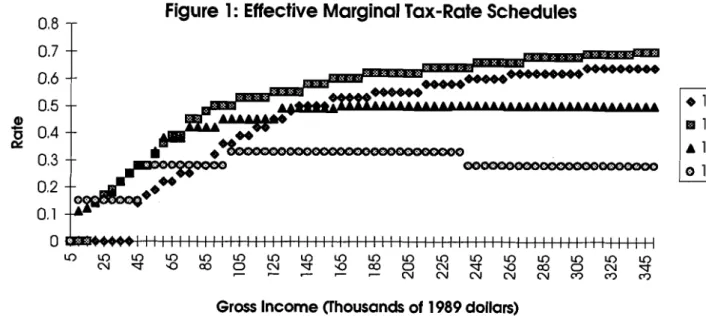
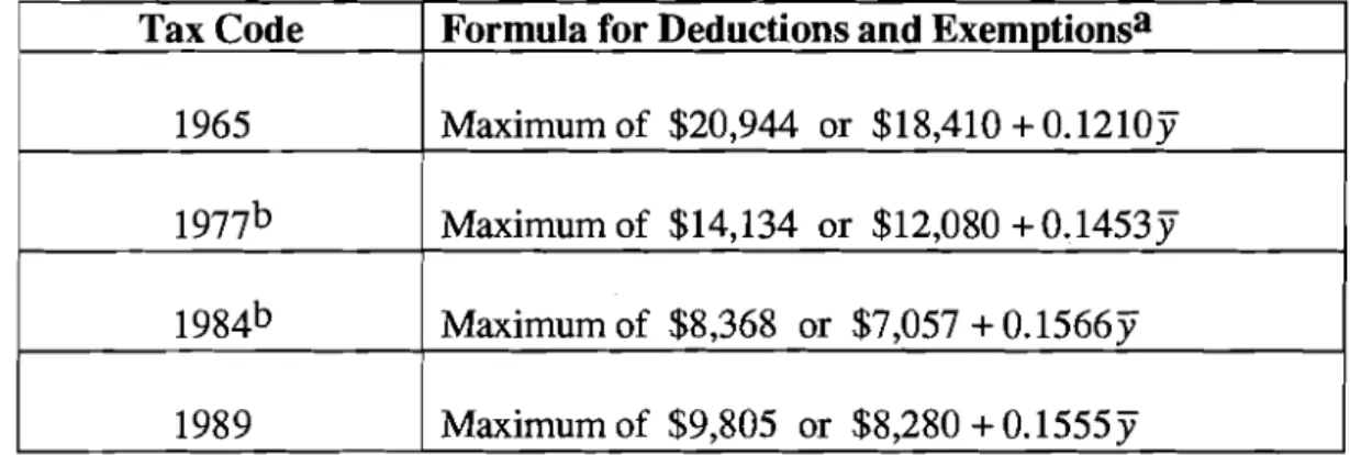
A broad sense of the separate rate structures we use is provided in figure 1, which plots effective marginal tax rates for incomes up to $350,000 (in 1989 dollars), with each tax code adjusted as explained above. (This value is in the range of the highest gross income obtained in our benchmark simulation.) Table 1 gives the estimated knctions for deduction and exemption adjustments for each of our four tax codes. Because standard deductions were incorporated into actual rate structures in tax years 1977 through 1986, the adjustment knctions used in simulations under the 1977 and 1984 codes are estimated from exemption levels only. However, to ease comparability, implied standard deductions

are included in the knctions for 1977 and 1984 shown in figure 1 and table 1.10

Finally, we note that, although the top marginal tax rate was 70 percent in 1977, different rates were applied to labor income and capital income, with the top rate on the former being, hypothetically, capped at 50 percent (see Lindsey [I98 11 and Slernrod [1993]).11 Adequate treatment of this and related issues would require modifLing the model to accommodate differential taxation of income from different sources, a task we do not undertake in this paper. However, as we report in section 4D, parallel experiments with back-of-the-envelope adjustments for this feature of the 1977 code suggest that none of our major conclusions is altered by ignoring these complications.

C. 7he Prodzrction Technology: Scaling the Model

Our simulation exercises assume that per capita aggregate product is given by

l o See Pechman (1987, appendix B) for a more thorough discussion of zero-bracket provisions in the personal income-tax code. The "standard deduction" levels and intercepts of the adjustment functions shown in table 1 are adjusted for inflation and real income growth.

In addition, variations in the treatment of capital gains introduced further distinctions in effective rate schedules for some taxpayers, as did the various payroll tax provisions in force during the years we are examining.

where 8 is capital's share in production and A is an arbitrary scale factor. Our benchmark

value for 8 is 0.36, and physical capital is assumed to depreciate 10 percent per period. Both of these choices are motivated by familiar long-run observations on capital shares (see, for example, the arguments in Kydland and Prescott [1982]). In addition, population growth is 1.3 percent per year, the postwar U.S. average.

Unlike many other calibrated simulation exercises, the scale factor A does play a

role in our experiments. In particular, because we are studying actual marginal rate brackets, it is necessary to scale the model such that generated incomes can be sensibly applied to the chosen tax codes. Essentially, we choose A so that the mean income

generated in the model's benchmark steady state equals the average gross income of joint filers in tax year 1989. In practice, matching the data in this way requires that the scale factor A and the intercept of the labor efficiency profile of the "richest" cohort (group 13,

described above) be chosen simultaneously.~2 D. Preferences

We specialize the utility hnction in equation (1) to the isoelastic form

where the preference parameters a and

a

represent the intertemporal elasticity of substitution of leisure and the utility weight of leisure, respectively. This formulation of preferences has the property that the capital-labor ratio is invariant to the scale factor A in

l2 It is possible to embed exogenous labor-augmenting technical progress into A, but we have chosen not to do so. While it is certainly easy, by a suitable change of variables, to solve the model with such an exqension, the notion of a steady state becomes solnewhat slippery when we contemplate both economic growth and the type of progressive tax systems that we are considering. In particular, in a growing economy with an unchanging tax code, all taxpayers will face the highest marginal tax rate in the long run. Thus, steady-state comparisons in our model implicitly assume that the relevant tax codes are indexed to real growth.

equation (lO).l3 We set o equal to 0.25, a choice motivated by a variety of empirical evidence culled from studies using disaggregated labor-market data. The parameter a is chosen such that steady-state hours worked by the "average" individual at peak

productivity are slightly greater than one-third of the total time endowment, which we take to be 16 hours per day. l 4

Most empirical studies find values for the subjective discount factor

P

in the neighborhood of 1 .O, sometimes slightly lower (for instance, Hansen and Singleton [1982]), sometimes slightly higher (for instance, Eichenbaum and Hansen [1990]). We choose a benchmark value of 0.99, which is consistent with satisfactory computed values of the long-run interest rate.

E. The Benchmark Equilibriunt

Our benchmark parameter choices result in a steady-state pre-tax real interest rate of about 3.04 percent (which is reasonably close to the apparent historical average of real pre-tax returns on long-maturity riskless bonds in the United States)15 and a steady-state l3 Scale invariance follows from the fact that changes in the level of wages have offsetting income and substitution effects on individual labor-supply decisions. (This property is also exploited in real business cycle models with positive rates of labor-augmenting technical progress. See, for instance, King, Plosser, and Rebelo [1988]). Apart from this theoretical argument, evidence from state-level data reported by Beaudry and Wincoop (1992) suggests preferences that are logarithmic in consumption. Beaudry and Wincoop further claim (footnote 10) that they found no evidence supporting either nonseparabilities between consumption and leisure or the absence of time separability in consumption, results that generally support the specification in equation (17). However, unlike our model, their maintained model includes "rule-of-thumb" consumers, or individuals who do not behave according to the pure life-cyclelpermanent- income hypothesis.

l 4 Standard empirical studies provide estimates of the intertemporal elasticity of substitution in labor ( 77 ). Because leisure accounts for approximately two-thirds of the total time endowment, 77 w 2 0 .

Thus, our choice of o implies a labor elasticity of about 0.5. MaCurdy's (1981) study of men's labor supply suggests elasticities in the range of 0.1 to 0.45, a result that is largely confirmed in related studies (see Pencavel [1986]). Although our labor elasticity choice is at the high end of these estimates, Rogerson and Rupert (1991) argue that, because of corner conditions, estimates of the degree of intertemporal substitution obtained from conventional analyses of male labor supply are likely to be understated. Furthermore, despite greater disparity in estimates obtained from studies of female labor supply, there is broad agreement that the elasticity is higher for women than for men (see Killingsworth and Heckman [1986]). In any event, our quantitative results do not appear to be sensitive to the choice of o , as we show in section 4D.

l5 See Siegal(1992), who reports average rates for the 1800-1990 period. We note, for the record, that average real rates appear to differ significantly across subperiods. Specifically, real returns to long-term bonds averaged 1.46 percent over the period 1889-1978, but 5.76 percent outside that interval.

capital-output ratio of 2.8 (which corresponds closely to the ratio of total capital to GDP in the United States over the 1959-1990 period).16

In addition to matching these standard aggregate variables, our calibration exercise is designed to deliver congruence between the benchmark model's tax- and income-

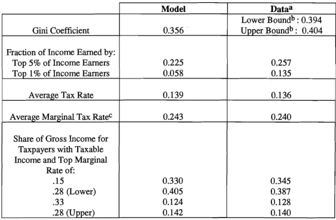
distribution characteristics with those derived from 1989 tax-return data. Some of the relevant comparisons along these dimensions are reported in table 2.

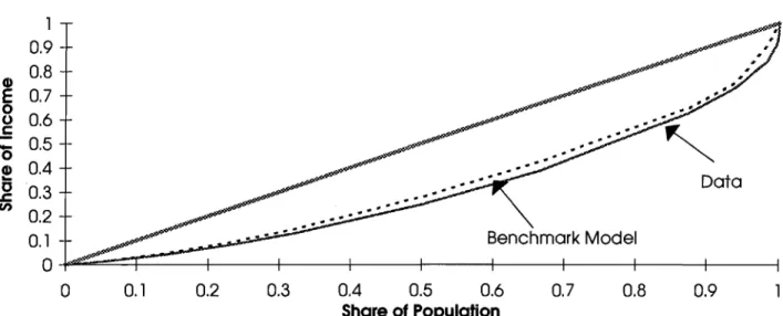
As indicated by the Gini coefficient, the distribution of income in the model is somewhat more equal than that exhibited by the data. This results in large part from the fact that, even after our adjustments to the Fullerton-Rogers estimates described above, the framework still underrepresents taxpayer incomes at the highest end of the

distribution. Although our simulations closely match the fraction of income earned by the top 5 percent of income earners

--

not surprising, since our calibration approach

essentially engineers this outcome

--

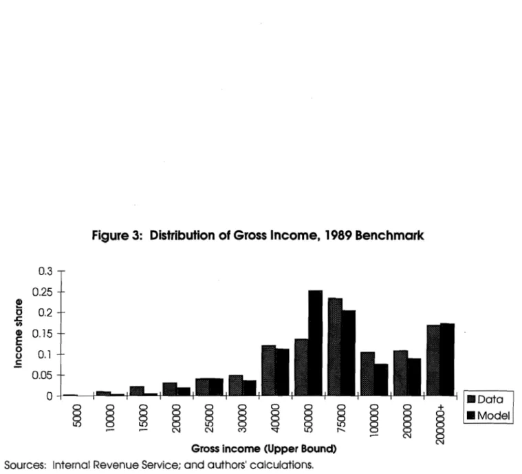
the share of the top 1 percent is less than half that found in the data. This difference is clearly illustrated by the Lorenz curves plotted in figure 2.

A more detailed view of the model's distributional features is found in figures 3 and 4, which compare actual and simulated distributions of gross income and taxes paid

according to the classifications provided in Statistics of Inconze. The most significant discrepancy between the two is the concentration of model income in the $40,000 to $50,000 range, a difference that is especially pronounced for gross income. The bunching of income in this range is partially a result of our scaling procedures, which focus on matching mean income in the model to that in the data.

As fbrther indicated by table 2, our benchmark model does quite well at matching the broad characteristics of the actual 1989 tax distribution: Simulated average and

l6 The measure used to construct the U.S. capital stock is the constant-cost net stock of reproducible

tangible wealth reported in the January 1992 Sulvey of Current Busir?ess. This measure includes consumer durables and government capital.

average marginal tax rates are virtually identical to the values derived from the data. Furthermore, the distribution of income generated by the model among the different marginal rate brackets is very close to that obtained from actual tax returns.

F. A Brief Comment on Solving the Model

Allowing for these discrete marginal tax-rate structures introduces certain

difficulties in computing the model solutions. In particular, straightforward application of the algorithms described by Auerbach and Kotlikoff (1987) requires continuous rate functions. However, because we are performing tax-compensated experiments, there exist alternative structures with continuous rate functions that generate the same equilibrium solutions as under our discrete rate functions, thus allowing application of the Auerbach- Kotlikoff methods. Details on these issues and our approach to solving the model appear in the appendix.

4. Income Tax Structure and the Distribution of Income: 1965-1989

Using the model calibrated to 1989 tax returns as a benchmark, our strategy is to compare actual changes in the distribution of income that occurred over the four years

1965, 1977, 1984, and 1989, with the tax-induced distributional changes implied by our quantified model. We focus on shifts in overall inequality as measured by the Gini coefficient, and in the share of pre-tax income earned by high-income taxpayers. Such changes can occur for several reasons: First, the income distribution can vary because of factors entirely unrelated to tax policy. Second, tax rules can change, adding or deleting feasible strategies for sheltering income. Third, changes in marginal tax rates can alter incentives to engage in existing shelter opportunities. Fourth, changes in marginal tax rates can alter individual labor-supply and saving decisions. Our approach here is designed to isolate variations in income distribution arising from this fourth cause.

A. Rate Structure and the Gini Measure of Inequality

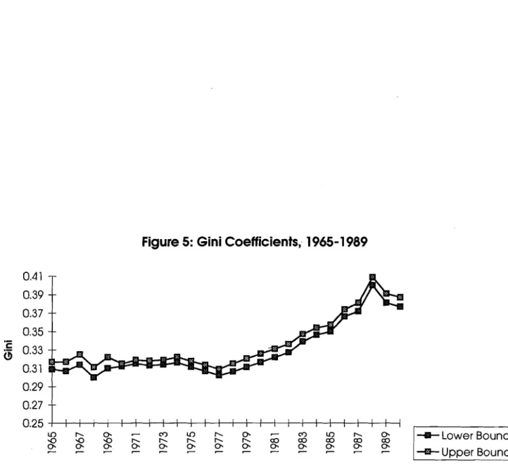
Figure 5 illustrates the time series of Gini coefficients for tax years 1965-1989, calculated from adjusted gross income figures reported in the Statistics of Income.17 The

observed trend in this inequality measure

--

relatively constant values through the 1970s followed by steady increases through most of the 1980s

--

matches that found in other studies of the same period using alternative data sets and examining different populations (see, for example, Karoly [1993]).

Table 3 lists the specific values of Gini coefficients for 1965, 1977, 1984, and 1989, along with the steady-state values calculated from the model under each year's tax regime. To make the comparisons somewhat more concrete, we also report a money metric for inequality suggested by Blackburn (1989). Comparing any two years (arranged in chronological order for convenience), the Blackburn measure provides the dollar amount of lump-sum tax in the initial year that must be taken from all individuals below the median income, and then transferred to all individuals above the median income, in order to generate the value of the Gini coefficient from the later year. In the calculations reported in table 3, a positive Blackburn value implies a greater degree of inequality under the 1989 tax code than under the relevant alternative.

Consider first the model outcomes. Arranged in "chronological" order, the

simulated Gini coefficients demonstrate a very pronounced U-shaped pattern over the four tax codes: The 1977 and 1984 rate structures, which produce nearly identical Gini

measures, generate less inequality than does the 1965 structure. The income distribution induced by the 1989 code is, in turn, identical to that under the 1965 code (in terms of the calculated Gini coefficient). Relative to either the 1977 or 1984 rate structures, both the 1965 and 1989 systems are equivalent, in distributional impact, to taking approximately

l7 Because of data limitations, the coefficient values for tax years 1975-1976 and 1979-1981 are

$2,500 from every taxpayer below the median income level and transferring the same amount to all those above the median.

How do these patterns match with the data? Contrasted with the U-shaped pattern exhibited in our simulations, the Gini coefficients extracted from the data evolved in a J-shaped fashion over the four years. In addition, the distributional changes seen in the data are much larger than those generated by the model.

This, of course, is entirely in line with expectations. Our experiments are not designed to explain distributional shifts in toto, but only those associated with the distortionary effects of changes in marginal tax rate functions. Furthermore, it is widely understood that inequality trends over the last two decades have been largely associated with nontax developments, an obvious candidate being the documented drift in wage differentials for skilled and unskilled labor (see, for example, Levy and Murname [1992]). The informational content of our experiments arises exactly from our ability to abstract from these "secular" trends, and therefore isolate the distributional consequences of the specific aspects of tax policy under consideration.

In addition, Levy and Murname argue that between-group income inequality

--

that is, inequality across different age, education, and gender groups

--

did decline modestly through most of the 1970s. However, this pattern was offset by increasing within-group inequality, leading to a relatively flat pattern in overall inequality measures. Because members of each age, j-type cohort are identical in our model, our experiments are closer in spirit to an examination of between-group inequality trends. Thus, the U- shaped behavior of Gini coefficients uncovered in our simulations is probably closer to the relevant pattern of actual inequality than is apparent from a simple comparison with figure

5.18

l8 Because the lifetime income cohorts are determined by their labor efficiency profiles, the j types can be usefully thought of as involving segregations of individuals according to education or skill levels.

Overall, our experiments do suggest that, if not for changes in U.S. tax policy, the trend toward greater income inequality would have been observed before 1977 (the year in which the Gini coefficient began its sustained upward trek). In this light, and conditional on the reasonableness of our artificial economy, table 3 suggests four major conclusions:

(1) None of the difference in the broad distribution of income in 1989 versus 1965 can be explained by hndamental differences in the structure of marginal tax rates.

Although inequality increased substantially across these two years

--

an increase in the 1965 Gini coefficient to the 1989 level would be equivalent to a (partial equilibrium) transfer of $9,662 from below-median to above-median taxpayers

--

all of the rise is due to nontax developments and/or changes in tax policy other than marginal rate differences.

(2) The effective rate structure in place in 1977 contributed to a greater degree of income equality than would have been realized under one that retained the characteristics of the 1965 code.19 Turning again to the Blackburn inequality measure, in the data we find that the decline in the Gini index from 1965 to 1977 can be translated into a monetary transfer of roughly $788 from above-median to below-median income earners.20 This amount is only about one-third of the difference implied by the model. Thus, we conclude that tax rate effects across these years exert a stronger influence on reducing inequality than would be apparent from a simple cut at the data that does not explicitly isolate the effect of tax policy.

(3) The marginal rate, exemption, and standard deduction changes associated with the Economic Recovery and Tax Act of 1981 explain virtually none of the substantial changes in income inequality between 1977 and 1984: Adjusted for inflation and income

l9 Recall that the 1965 structure differs from 1977 due to the effects of inflation and real income growth between the two years, as well as different treatment of exemptions and deductions.

20 This rough comparison does not provide a direct analysis of the income distributions in the two years, Because the money value of the implied transfer depends on the mean of the reference distribution, direct application of Blackburn's arguments 111ould require choosing either 1965 or 1977 as the base year.

growth, the 1977 and 1984 structures generate virtually identical values for the Gini coefficient.

(4) The effective rate structure of the Tax Reform Act of 1986 appears to have had a substantial effect on income distribution: Our simulations indicate that changes in labor-supply and saving decisions induced by the elements of the 1986 tax reform that we study can explain 46 percent of the difference in the Gini between 1984 and 1989, and 42 percent of the difference in the Blackburn index.

Three hrther comments regarding point (4) are in order. First, the comparison is not exact because of our adjustments for nominal income. However, the relatively short time between these two years minimizes the differences between the nominal rate structures faced by households and the adjusted schedules used in our experiments.

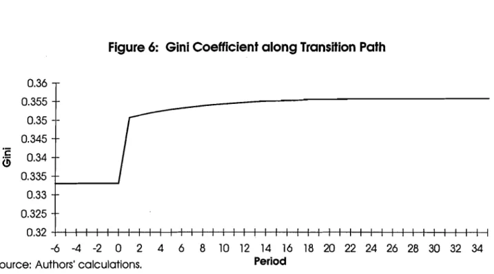
Second, the results reported in this section are based on steady-state analysis. Thus, the claim that the model captures 46 percent of the difference in the Gini between 1984 and 1989 requires that the dynamic behavior of the inequality measure is such that it converges rapidly to its steady-state value. In fact, as shown in figure 6, this is indeed the case: In the period of an unanticipated shift from the 1984 tax regime to the 1989 regime, the Gini rises to 98.5 percent of its new steady-state value.

Third, there is some evidence, summarized in Blank and Blinder (1986), that inequality is countercyclical. This research is relevant because output growth was significantly lower in 1989 than in any of the other three years from which our tax structures are taken. (The annual growth rate of GDP was 5.6,4.5, and 6.2 percent in, respectively, 1965, 1977, and 1984, but only 2.5 percent in 1989.) In light of this, our "snapshot" examination of the actual Gini coefficients may overstate the inherent (cyclically adjusted) degree of inequality in the 1989 data, and hence understate the fraction of the change in inequality that is captured by our model.

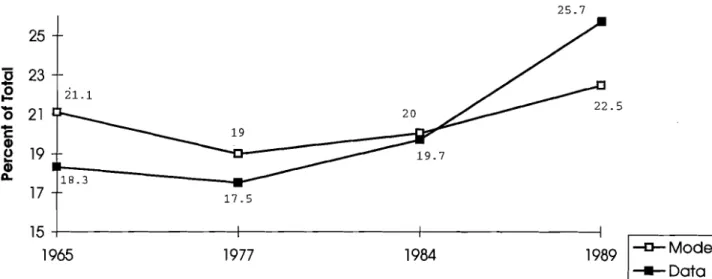
B. Rate Structure and the Share of High-Inconie Tmcpayers

Because reductions in top marginal tax rates constituted one of the most dramatic changes implemented by the Tax Reform Act of 1986, a good deal of recent research on tax policy has concentrated on changes in the income share received by high-income taxpayers. The general conclusion from such investigations

--

several of which are cited in the introduction to this paper

--

is that the 1986 legislation induced a marked increase in these shares.

Figure 7 reports the income shares of the top 5 percent of taxpayers, from both the data and our model simulations, for each of the years we consider.21 With respect to the general tendencies found in the tax-return data, the model successfblly predicts the general shape in the path of these income shares over time. However, as with the overall

distributional picture painted by our examination of trends in the Gini index, the distortionary impact of the tax rate structure can account for only a fraction of the

observed increase in concentration at the top of the income distribution. Still, that fraction is substantial. Our simulations indicate that between 1984 and 1989, for example, almost half of the increased share of pre-tax income earned by the top 5 percent of earners can be attributed to the effects of changes in leisure and consumption incentives brought about by tax reform.

C. Rate Structure and the Distribution of Lifetime Income

Over the life cycle, of course, any given household

--

both in our model and in the real world

--

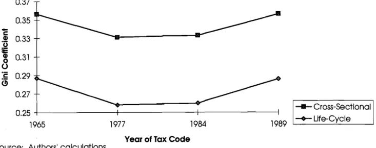
realizes many different levels of income and faces several distinct marginal tax rates. Although it is widely acknowledged that the distributional consequences of 21 Many recent studies of the 1986 tax reform have focused on the behavior of "very h i g h income recipients, typically the top 1 percent of taxpayers. Recall from section 3 that to incorporate high-income individuals into our model, we extrapolate from the Fullerton and Rogers (1993) estimates in such a way that the benchmark steady state matches the top 6 percent of the income distribution. A consequence of this approach is that we underestimate the share of income of the top 1 percent of taxpayers. In 1989, for example, the highest 1 percent among married persons filing jointly earned 13.5 percent of reported adjusted gross income on taxable returns. In contrast, the same group earns 5.8 percent in our model. Therefore, our discussion of high-income taxpayers is best suited to a consideration of the top 5 percent.

particular tax systems from a life-cycle perspective may be inadequately captured in analyses of cross-sectional income, previous studies have failed to uncover dramatic differences in the patterns of lifetime vs. annual tax incidence (see, for instance, Davies, St-Hilaire, and Whalley [I9841 and Fullerton and Rogers [1991]).

Similarly, we find in our experiments that the relative impact of the different tax regimes on lifetime income distributions is comparable to that found in our previous analysis of cross-sectional income. Although the Gini coefficient values calculated from lifetime income groupings are uniformly lower than those calculated in the standard way, they exhibit the same U-shaped pattern over the four tax codes (see figure 8). Lifetime income here is simply the present value of labor income, which, given the structure of our model, is equivalent to wealth.

Interestingly, inequality shifts resulting from tax structure changes are slightly

more pronounced in the lifetime income distribution than in the cross-sectional

distribution: The changes in Gini coefficients, in both absolute and percentage terms, are larger when calculated on the basis of wealth than when calculated from cross-sectional income. Thus, our results would contradict an argument suggesting that rising inequality associated with recent tax reforms is mitigated when life-cycle income mobility is explicitly incorporated.

D. Some Sensitivity Analysis

In table 4, we report steady-state values for Gini coefficients calculated under alternatives to our benchmark parameterization. Specifically, table 4 includes results for separate simulations that differ fiom the benchmark experiments because of (i) an assumed labor-supply elasticity toward the lower end of the range estimated from microdata, (ii) changing the intercept in the pre-1989 adjustment fbnctions such that all structures yield the same total steady-state revenue, (iii) eliminating the real income growth correction for

the pre-1989 rate structures, and (iv) incorporating the maximum tax rate for earned income into the assumed rate structure for 1977.22

As table 4 suggests, our previous conclusions are robust to these alternative treatments. In particular, the Gini inequality measures are not much affected by these variations, and comparisons across the four rate structures reveal the same U-shaped pattern seen in table 3 and figure 7. (Note, however, that the pattern for the cases where the codes are not adjusted for real income growth more closely resembles the J-shaped behavior found in the data.)

5. Tax Revenue and Rate Structure: Static versus Dynamic Analysis

The results reported in the previous section demonstrate empirically significant adjustments of individual labor-supply and saving decisions in response to historically relevant changes in marginal tax rates. Corresponding to these adjustments, of course, are changes in the revenues collected from the affected individuals.

Table 5 summarizes the steady-state equilibrium tax characteristics derived from simulations under each of the tax codes. Consider, specifically, the experiments performed with the 1977 and 1989 rate structures. Although the former regime yields a higher mean tax rate, higher marginal tax rates (on average), a higher top marginal rate, and generally greater progressivity toward the upper part of the income distribution, the aggregate revenue collected under the 1977 system is slightly lower than obtained under the 1989 code. This observation invites a provocative conclusion: Relative to some nontrivial alternatives, reductions in marginal tax rates of the magnitude implemented by the Tax Reform Act of 1986 are capable, through private factor supply decisions alone, of

22 For variation (ii), we search over values of the income-adjustment-function intercept (described in section 3B) until aggregate steady-state revenue equals the steady-state revenue obtained in the 1989 benchmark case. For variation (iv), we replace the statutory rates in the 1977 code that exceed 50 percent with their corresponding "average marginal rates with maximum tax," as reported in table 3.3 of Slemrod (1993).

expanding the tax base sufficiently to yield higher revenues. In other words, our results suggest the existence of a "Laffer curve" in the relevant region of U.S. history.

The problem in interpreting the information provided in table 5 is, of course, that for most taxpayers

--

including those at the top of the income distribution

--

the different tax structures we consider involve changes in both marginal and inframarginal tax rates. Although mixing the effects is legitimate in the context of examining each of the separate rate structures in their totality, the inframarginal changes tend to obscure discussion of the nexus between actual tax reforms, economic incentives, and aggregate tax revenue.

However, a fairly direct way to isolate the effect of behavioral distortions of specific changes in marginal rate structures is available in our framework by comparing "static" versus "dynamic" revenue outcomes. In other words, for each pre-1989 tax code, we compute static revenue outcomes by applying the 1989 rate structure to the fixed equilibrium values of consumption and leisure choices under that alternative. If the

distortionary impact of marginal tax rate changes has a quantitatively significant impact on tax collections, these static calculations will yield aggregate revenue levels that are quite different from their dynamic general equilibrium counterparts.

Table 6 provides the results of experiments that directly address this question. The numbers reveal a significant divergence between the static and dynamic outcomes. For example, under static assumptions, shifting from the 1965 to the 1989 code would raise aggregate revenues by just over 40 percent in the long run. The actual dynamic outcome, which incorporates the distortionary impact on individual behavior, indicates that the increase would be only 36 percent.

Because the overall revenue implications of the 1977 and 1984 codes are much closer to the 1989 benchmark, the discrepancy between the static and dynamic

experiments stands in sharper contrast. In the case of shifting fi-om the 1984 alternative to the 1989 structure, long-run revenue losses under static assumptions are almost 90 percent higher than those realized in full general equilibrium. For the 1977 alternative, static

assumptions indicate a revenue loss of 6.6 percent, while the analogous dynamic

calculations indicate that shifting to the 1989 rate configuration generates a slight gain in aggregate revenue.

To put some perspective on the magnitude of these differences, individual income tax collections in 1984 totaled approximately $356 billion (in 1989 dollars). Given this figure, the implied discrepancy between the static and dynamic experiments reported in table 6 amounts to a long-run annual revenue shortfall of about $23.5 billion.23

7. Income Tax Structure and Economic Welfare

Ultimately, we wish to know how tax structure affects measures of economic welfare. In this section, we examine the utility losses and gains associated with the

previously discussed tax-induced changes in income inequality. For brevity

--

and because it represents the experiment that most closely replicates the U.S. experience under the Tax Reform Act of 1986

--

our focus will be on comparing the 1984 and 1989 rate

structure^.^^

For any individual living in a long-run equilibrium under the 1984 tax structure, we calculate the welfare loss of shifting to the 1989 tax system as the percentage decrease in full wealth

--

defined as the present value of labor income when the individual's entire time endowment is allocated to market work

--

that is necessary to maintain utility at its initial level. Negative numbers thus represent cases in which lifetime utility is higher under the

1989 tax structure, and positive numbers those in which lifetime utility is higher under the alternative structure.

23 This number, of course, abstracts from the effects of income growth.

24 The results reported in this section do not adjust for the fact that the 1984 and 1989 structures imply different levels of total revenue from the income tax. However, all of our primary results obtain when steady-state revenues are equalized by adjusting the level of the standard deduction, as described in section 4D. Although this procedure alters marginal tax rates for a small number of individuals at the very bottom of the income distribution, these parallel experiments leave intact the shape of the rate structures themselves. Thus, the conclusions described in this section also apply to analogous revenue-neutral tax reforms.

The welfare results for each of the 13 lifetime income groups are depicted in figure 9. The average (population-weighted) welfare loss associated with changing from the

1984 to the 1989 structure averages -0.63 percent of full wealth. In other words, the average household gains by a shift to the rate structure implied by the Tax Reform Act of 1986. However, as is clear from figure 9, this average masks a wide range of outcomes for the individual lifetime-income cohorts. The very wealthiest group (cohort 13) enjoys a welfare gain from tax reform equivalent to a full 2.1 percent of its wealth. Cohort 2, on the other hand, suffers an equivalent wealth loss of 0.4 percent.25

The pattern of utility effects harbors no surprises when one compares the two marginal rate schedules (see figure 1). After our adjustments for inflation, real growth, and differences in deductions and exemptions, the 1989 code entails lower rates on most gross incomes above $56,000. These income levels are primarily relevant for lifetime income groups 10- 13

--

exactly the groups that would experience welfare gains.

This rather unsurprising outcome repeats itself across all experiments comparing the different rate structures: Higher marginal tax rates over the life cycle tend to reduce lifetime utility. For instance, tax rates from the 1977 code are very similar to those of

1989 up through gross incomes of about $80,000. At the highest income levels, however, rates from the former substantially exceed those from the latter. Consequently, whereas the replacement of 1977 rates with 1989 rates has little impact on most households, the effect is substantial for the "rich," equaling gains of 0.5 percent and 2.8 percent ofwealth for cohorts 12 and 13, re~pectively.~G

25 The 1984 steady-state income of cohort 2 ranges from about $5,000 to $25,000, with an average of about $20,000. It should be noted again that the welfare effects in our experiments are due only to the substitution effects resulting from the tax changes. Although the shift from the 1981 to the 1989 tax code results in welfare losses for cohorts with low lifetime incomes, these groups actually pay less in total tax

revenues under the latter code. Because revenues are returned to individual agents in a lump sum, our welfare numbers do not reflect whether any taxpayer would be better or worse off when changes in tax

liabilities are included. In future work, we plan to examine this issue in variations of the model where tax

receipts are not rebated in lump sum.

These welfare results are almost entirely driven by the changes in tax structure per se, as opposed to general equilibrium effects on factor prices induced by these changes. Figure 9 also reports the results of partial equilibrium experiments, referred to as the "tax effect only" case, in which we fix the aggregate wage and interest rate at their initial steady-state values, then calculate individual consumption and leisure paths under the 1989 tax code with these fixed aggregate prices.27 As shown, both the qualitative and quantitative outcomes are similar to those obtained from the full general-equilibrium simulations.

Finally, figure 10 shows, for selected lifetime income groups, welfare losses along the transition path for the representative case of a shift from the 1984 to the 1989 tax code. As before, we suppose that the regime change occurs at time 0 and is unanticipated. Consistent with the observation that general equilibrium effects have little impact on welfare outcomes, the utility consequences for agents who become economic adults on or after the date of the tax reform are virtually identical to those found for the steady state. Losses and gains for individuals already alive at the time of the change tend to decrease monotonically in age, as illustrated by the patterns of lifetime income for group 2 (the second "poorest" of the groups, and the one that suffers the largest loss from the shift to the 1989 code) and group 13 (the "richest" group, and the one that enjoys the largest gain from the shift). Group 8, a middle-income group, is an exception, although the welfare effects for this cohort are generally trivial.

9. Concluding Remarks

Our analysis supports a largely unconfirmed suspicion about the recent evolution of tax policy: The marginal rate changes implemented in various tax reforms over the past several decades are capable of explaining much of the change in U.S. income distribution experienced during that time.

27 Full wealth and the valuation of consumption and leisure paths

--

and, hence, our welfare measure

--

are also calculated assuming the initial interest rate and wage.

We emphasize that these observations pertain to the distribution ofpre-tax income. Karoly (1 993), for instance, has argued that ". .

.

it seems fair to conclude that the rise in pre-tax inequality dominates any increase in post-tax inequality due to a reduction in the progressivity of the tax system during the 1980s." While our results do not contradict this statement, they do suggest a renewed emphasis on the role of progressivity in the

determination of the gross-income distribution.

We also find that tax-created increases in income inequality correspond to rising "utility inequality": The highest lifetime income group gains in both income share and utility from the 1989 tax structure. The lowest lifetime income group, on the other hand, suffers utility losses and would prefer any of the other alternatives.

The welfare effects for the "poorest" lifetime income groups are particularly interesting for the experiments with the 1977 and 1984 alternatives because these groups lose utility from a shift to the 1989 regime, even though aggregate income increases. Thus, general equilibrium spillover effects from the lower rates for top incomes in the

1989 code

--

effects that are, somewhat lamentably, referred to as "trickle down" in popular jargon

--

are not sufficient to improve the welfare'of those at the bottom of the income distribution. However, we emphasize that welfare improvements for the "winners" under the 1989 tax structure are very large relative to the resulting welfare reductions of the "losers." Although we have not explicitly calculated equilibria with transfer schemes that preserve the utility levels of this latter group, it is clear that such Pareto-improving policies e x i ~ t . 2 ~

Generally, our results confirm the substantial effects that real-world rate differentials can be expected to have under sensible assumptions about household substitution elasticities. Not surprisingly, we do not generally find that, viewed in its 28 A usual procedure is to consider a set of lump-sum transfers as a compensating scheme (as, for instance, in Auerbach and Kotlikoff [1987]). An interesting, and more realistic, alternative would be an

expansion of earned-income credits offset by other (distortionary) adjustments for higher-income individuals. We plan to examine this issue in future work.

entirety, the 1989 rate structure could plausibly be expected to deliver increased revenues. Nonetheless, the behavioral responses to rate changes are large, and the model testifies to the importance of dynamic analyses of contemplated tax reforms.

References

Auerbach, Alan J. and Laurence J. KotlikofT, Dynanzic Fiscal Policy, Cambridge University Press: New York, 1987.

Beaudry, Paul and Eric van Wincoop, "Alternative Specifications for Consumption and the Estimation of the Intertemporal Elasticity of Substitution," Discussion Paper 69, Institute for Empirical Macroeconomics, Federal Reserve Bank of Minneapolis, July 1992.

Benveniste, Lawrence M. and Jose A. Scheinkman, "On the Differentiability of the Value Function in Dynamic Models of Economics," Econonzetrica, 47, 1979, 727-32. Blackburn, McKinley L., "Interpreting the Magnitude of Changes in Measures of Income

Inequality," Journal of Econonzetrics, 42, 1989, 2 1-25.

Blank, Rebecca M. and Alan S. Blinder, "Macroeconomics, Income Distribution, and Poverty," in Fighting Poverty: What Works and What Doesn 't, Sheldon H. Danziger and Daniel H. Weinberg, eds., Harvard University Press: Cambridge, MA, 1986, 180-208.

Davies, James, France St-Hilaire, and John Whalley, "Some Calculations of Lifetime Tax Incidence," American Economic Revie~v, 74, 1 985, 63 3 -49.

Eichenbaum, Martin and Lars Peter Hansen, "Estimating Models with Intertemporal Substitution Using Aggregate Time Series Data," Jozrrnal of Business and Econon~ic Statistics, 8, January 1 990, 53 -69.

Feenberg, Daniel R. and James M. Poterba, "Income Inequality and the Incomes ofVery High-Income Taxpayers: Evidence from Tax Returns," in Tax Policy and the Econonly, James M. Poterba, ed., 1993.

Feldstein, Martin, "The Effect of Marginal Tax Rates on Taxable Income: A Panel Study of the 1986 Tax Reform Act," NBER Working Paper No. 4496, October 1993. Fullerton, Don and Diane Lim Rogers, "Lifetime Versus Annual Perspectives on Tax

Incidence," National Tax Jozmml, 44, September 199 1,277-87.

Fullerton, Don and Diane Lim Rogers, Who Bears the Lifetinze Tax Burden?, The Brookings Institution: Washington, D.C., 1993.

Gastwirth, Joseph L., "The Estimation of the Lorenz Curve and Gini Index," Review of Econonzics and Statistics, 54, 1972, 320-22.

Hansen, Lars Peter and Kenneth J. Singleton, "The Generalized Instrumental Variables Estimation of Nonlinear Rational Expectations Models," Econornetrica, 50, February 1982, 1269-86.

Karoly, Lynn A., "Trends in Income Inequality: The Impact of, and Implications for,

Tax

Policy," in T m Progressivity, Joel Slemrod, ed., Cambridge University Press: New York, 1994, pp. 95-129.

Killingsworth, Mark and James Heckman, "Female Labor Supply: A Survey," in Handbook of Labor Economics, vol. 1, 0. Ashenfelter and R. Layard, eds., North-Holland: New York, 1986.

King, Robert G., Charles I. Plosser, and Sergio T. Rebelo, "Production, Growth, and Business Cycles," Journal of Monetary Economics, 2 1, MarchMay 1988, 195- 232.

Kydland, Finn E. and Edward C. Prescott, "Time to Build and Aggregate Fluctuations," Econornetrica, 50, 1982,50-70.

Levy, Frank and Richard J. Murname, "U. S. Earnings Levels and Earnings Inequality: A Review of Recent Trends and Proposed Explanations," Journal of Economic Literature, 30, September 1992, 1333-8 1.

Lindsey, Lawrence B., "Is the Maximum Tax on Earned Income Effective?" National T m

Journal, 34, 1981, 249-55.

Lindsey, Lawrence B., "Individual Response to Tax Cuts: 1982-1984," Journal of Public Economics, 33, 1987, 173-206.

Lindsey, Lawrence B., The Growth Experiment, Basic Books: New York, 1990. Lindsey, Lawrence B., "A Reconsideration of Graduated Tax Structures," unpublished

manuscript, Board of Governors of the Federal Reserve System, Washington, D.C., 1993.

MaCurdy, Thomas, "An Empirical Model of Labor Supply in a Life-Cycle Setting," Journal of Political Econonzy, 89, 198 1, 1059-85.

Pechman, Joseph A., Federal T m Reform, fifth edition, The Brookings Institution: Washington, D.C., 1987.

Pencavel, John, "Labor Supply of Men: A Survey," in Handbook of Labor Economics, vol. 1, 0. Ashenfelter and R. Layard, eds., North-Holland: New York, 1986.

Rogerson, Richard and Peter Rupert, "New Estimates of Intertemporal Substitution: The Effect of Comer Solutions for Year-Round Workers," Journal of Monetary Econon~ics, 27, April 199 1, 255-69.

Siegal, Jeremy J., "The Real Rate of Interest from 1800-1990: A Study of the U.S. and the U.K.," Journal of Monetary Economics, 29, April 1992, 227-52.

Slemrod, Joel, "On the High-Income Laffer Curve," Working Paper No. 93-5, Office of Tax Policy Research, University of Michigan, March 1993.

Appendix: A Note on Solving the Model

Although our model is similar in most respects to the structures pioneered by Auerbach and Kotlikoff (1987, for example) and extended by Fullerton and Rogers (1 993), the solution techniques are complicated by allowing for discontinuous tax codes that imply nondifferentiable budget surfaces. Fortunately, it is possible to construct artificial continuous tax codes that yield the same first-order conditions as the model with a discrete marginal tax-rate structure, which in turn allows a straightforward application of the algorithms described by Auerbach and Kotlikoff

To outline the general approach, suppose that we have a simple two-bracket tax code given by

which holds for all j-type agents, at all ages t, and all times s. Relative to a more standard case with a continuous marginal tax-rate function, the optimization problem confronting an individual facing the discrete tax code in (Al) differs by the addition of the constraint

When this constraint binds, jjlS =

7,

and, suppressing the time subscripts s for convenience, the first-order necessary conditions are

and

where, for all j types, u:, denotes the age t marginal utility of consumption (i=c) and leisure (i=Z),

iZ',

is the LaGrange multiplier associated with the budget constraint in equation (2) of the text, and ,u: is the LaGrange multiplier associated with the constraint in equation (A2).

It is straightforward to veriQ that there exists a continuous marginal tax-rate finction with rates given by

that also satisfies the necessary conditions (A3)-(A5). Because we perform only tax- compensated experiments, the equivalence of the first-order conditions is sufficient to guarantee the equivalence of equilibrium outcomes. Thus, our solution approach essentially involves replacing discrete rate structures, as in (Al), with alternative continuous codes similar to those implied by (A6).

To sketch the proof demonstrating the validity of this replacement, note that the hypothetical continuous rate structure is identical to the actual tax code when the

conditions ( r

,

= r L , y: < y"} or ( r , = r H , y: > y"} are satisfied. Thus, we will focus on the case where the constraint ( r , - rH)@:

-7)

2 0 is binding. For simplicity, we discuss only the steady state, recognizing that transition-path solutions are directly analogous under the assumption of perfect certainty.

where G(a) denotes the transition equations defined by the budget constraints in equation (2) of the text, a * is the asset choice that solves

V(a) r max (rr(c, 1)

+

@'(a1)),

~ ~ 1 . a

and a' represents next period's asset choice.

Because u(.) is concave, W(a), is concave. Furthermore, W(n) is continuously differentiable if its derivative, W1(a), exists and is continuous. If W1(a) is continuous, then V1(a) is continuous (see Benveniste and Scheinkman [1979]). To demonstrate the continuity of W'(a), we need to consider points at which y* =

y

.

That is, we must show that, at the indifference points where

?

= r

'

and

i

= r ,

wNB1

(a*) =

w,'

(a*), where B indicates that the constraint is binding and NB indicates that it is not.

By definition,

7

= ntl[l- l(a* )]

+

ra* when the income constraint binds. Thus, differentiating (A7) and substituting from this constraint and the first-order conditions gives

1 d~

dl

WNB

( a * )

= uc

-+

u, -

da da

Similarly, by exploiting the first-order conditions for the unconstrained case, we obtain