Receptivity on an Airfoil
W. Wurz1, S. Herr1, A. Worner1, U. Rist1, S. Wagner1 and Y. S. Kachanov2
1 Institut fur Aerodynamik und Gasdynamik (IAG), Universitat Stuttgart, Pfaenwaldring 21, 70550 Stuttgart, Germany
2 Institute of Theoretical and Applied Mechanics (ITAM), Russian Academy of Science, 630090 Novosibirsk, Russia
Abstract. Hot-wire measurements are perfomed on linear 3D acoustic receptiv-ity in a two-dimensional laminar boundary layer. A localized quasi steady surface roughness serves as the receptivity element. A plane acoustic wave with frequency f
ac scatters at this vibrating source and the generated TS-wave train is measured downstream in spanwise cuts and at combination frequencies (f1
2=
fac fv). After Fourier decomposition linear stabiltity theory is used for upstream extrapolation to the initial amplitudes at the roughness element. The dispersion characteristic is de-termined and the complex receptivity function is calculated by normalization of the initial TS-spectra with the related amplitudes and phases of the surface vibrator and the acoustics. The results are compared with Direct Numerical Simulations based on a vorticity-velocity formulation of the complete Navier-Stokes equations and a new embeded wall model. Good overall agreement is achieved.
1 Introduction
The problem of boundary layer transition from laminar to turbulent ow still attracts much attention because of its fundamental and practical importance. It has three main aspects. First, there is the laminar ow receptivity to ex-ternal perturbations. The second aspect is the linear development of bound-ary layer instabilities according to linear stability theory and nally there is the nonlinear ow breakdown to turbulence. This paper is devoted to exper-imental and numerical investigations of the linear 3D acoustic receptivity of a two-dimensional laminar boundary layer in the presence of a localized (3D) quasi steady surface non-uniformity.
This problem is poorly studied, so far. Most of the previous experiments in this eld were devoted to two-dimensional receptivity problems (see e.g. 1], 2]). The quantitative receptivity characteristics of the 2D (Blasius) boundary layer to 3D surface vibrations were studied experimentally in 3]. The only available experimental investigation of the 3D vibrational acoustic receptivity was carried out in a swept-wing boundary layer and was devoted to the generation of cross-ow instability modes 4].
In general, the amplitude part of the acoustic receptivity coecient is dened by the ratio of the initial (i.e. at the surface non-uniformity) instabil-ity wave amplitude, generated in the boundary layer, to the amplitude of the
external acoustic perturbation and the amplitude of the involved surface non-uniformity 5], 6], 4]. More exactly, all these amplitudes must be determined for every single (normal) mode of the corresponding frequency-wavenumber spectra, i.e. the spectra of the instability waves, surface non-uniformities and acoustic perturbations.
2 Experimental Investigation
The experiments were carried out in the Laminar Wind Tunnel (LWT) of the IAG. The LWT is an open return tunnel with a turbulence level less thanTu= 2 10;4. The boundary layer measurements were performed on a symmetrical airfoil section at zero angle of attack and at a Reynolds number of 1:2 106based on the arclengths
max= 0:615mmeasured from the leading
edge. A plane acoustic wave with xed frequency (fac = 1088Hz) close to
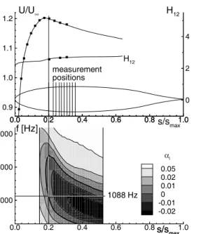
the most unstable TS-frequency was chosen as the external perturbation. The acoustic wave was generated by a loudspeaker at the centerline downstream of the test section. The position of the 3D roughness was selected to lie on branch I for the investigated frequency (Fig. 1).
When studying 3D roughness acoustic receptivity, the data analysis rep-resents a very complicated problem because of diculties to distinguish sig-nals measured at the same (acoustic) frequency but having dierent physical nature. The signal consists of a mixture of: (i) the instability wave generated by the acoustics (that is relatively weak initially), (ii) vibrations of the hot-wire probe and the model surface, and (iii) the acoustic eld itself including the Stokes layer in the near-wall region. These experimental problems have been solved in 4] by means of arranging an unsteady surface non-uniformity (vibrating source) oscillating with a very low frequency and providing a quasi-steady scattering of the acoustic wave. A similar method has been applied in the present investigation. The vibrating source is driven at the frequency
fv = 1
64 fac which leads to an amplitude modulation of the generated 3D TS-wave in time. This corresponds to distinct combination modes in the fre-quency spectrum of the hot-wire signal at frequencies (f12 =fac
fv). In contrast to the signal observed at the acoustic frequency, the combination harmonics correspond to the instability waves only. The spatial behavior of these combination modes has been studied in detail.
The 3D roughness element was modeled by the inection of the membrane of a circular surface vibrator. The active diameter (6mm) was chosen to be approximately one half of the TS-wavelength (atfac). The body of the
source (Fig. 2) was set up ush-mounted with the model surface. The vinyl membrane was driven by a loudspeaker and the shape of the inection of the membrane was measured with a laser triangulation device (Fig. 2).
An acoustic amplitude of 100dB was used together with a vibrational amplitude of 29:7 mRMS in order to be in the linear regime of receptivity
and linear development of boundary layer instabilities.
The acoustic frequency as well as the vibrational frequency and the sampling trigger were generated strictly phase locked by a single time source. The
ra-tios between the frequencies were chosen as integer powers of two (fv:fac:
fsample= 1 : 64 : 8) which gave the possibility to represent each of them with
Fourier coecients after a single FFT.
The initial amplitudes of the most unstable TS-waves (which are neces-sary for determining the receptivity coecients) can not be measured dir-ectly in the ow because in the near-eld of the source a mixture of dier-ent other perturbations such as continuous-spectrum instability modes and forced (bounded) uctuations is present. Therefore, similar to some previ-ous receptivity experiments (see e.g. 3]), we used the boundary layer as a selective amplier of the most unstable (discrete-spectrum) modes and, sim-ultaneously, an attenuator of the continuous-spectrum modes and the forced oscillations. The distributions of the TS amplitudes and phases were meas-ured downstream of the surface non-uniformity. In contrast to 3] the linear stability theory was then used for extrapolation of the data to the position of the surface non-uniformity.
The hot-wire measurements were performed in 8 to 9 spanwise scans cov-ering the whole width of the wave train. The time signals at every measure-ment point were analyzed with an FFT and the amplitude and phase of the perturbations obtained at the combination frequencies (f12) were used for further data processing. The amplitudes were normalized by the local free-stream velocity U = 36ms and the length with the displacement thickness
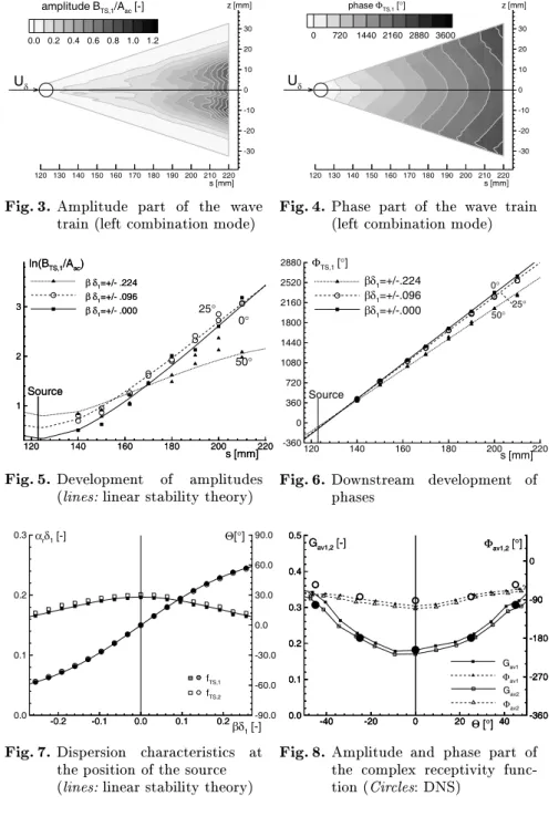
1ref = 0:356mm(H12 = 2:57) at the position of the source. The resulting spatial elds of the disturbance amplitude and phase for the "left" combina-tion mode (f1=fac
;fv) are shown in Fig. 3 and Fig. 4, respectively.
3 Experimental Results
The complex values of the wave train in physical space were mapped for each spanwise cut to spanwise wavenumber spectra. After this the downstream development of waves with dierent spanwise wavenumbers were investigated separately. The measured amplitudes (Fig. 5, symbols) amplitudes for the combination modes are found to be consistent with the linear stability theory (Fig. 5, solid lines).
This allows an upstream extrapolation to the position of the receptivity element. The associated phases Fig. 6 can easily be t by a straight line. The gradient of this line is the streamwise wavenumberr. By this procedure the
dispersion characteristicr=r() is determined that gives a dispersion
re-lationship between the streamwise and spanwise wavenumbers (Fig. 7). From the double Fourier decomposition of the shape of the membrane oscillation the complex wavenumber spectrum of the surface vibration is obtained. From this spectrum the amplitudes of the "resonant" vibrational modes, that have the same wavenumbers as the TS-waves generated by them, can be found with the help of the dispersion function. Thus, the complex receptivity func-tionGe
av12(r) can be evaluated by calculating its amplitude part and its phase part separately according to the following denition
e Gav12(r) =Gav(r) e iav 12 ( r )= e BinTS12 ( r ) e Aac Ae v ( r )
where BeinTS is the complex initial spectrum of TS-waves excited by the acoustics on the vibrator,Aeacis the complex acoustic amplitude, andAev(r) is the complex spectrum of the resonant vibrational modes. Figure 8 shows the amplitude and phase parts of the complex receptivity functions in depend-ence of the propagation angle() = arctanr of the generated TS-wave for the two combination frequencies studied.
4 Comparison with Direct Numerical Simulations
The DNS are based on the vorticity-velocity formulation of the complete Navier{Stokes equations using a uniformly spaced grid in streamwise and wall-normal direction and a spectral representation in spanwise direction, c.f. 7]. The sound wave in the free stream is prescribed as a solution of the second Stokes' problem at inow, and a novel wall model has been implemen-ted and compared with standard rst-order formulations that consider only a no-slip condition in wall-parallel directions. The use of a body-tted coordin-ate system is avoided and the typically small surface roughness is simulcoordin-ated by non-zero velocity at the lowest row of grid points which are extrapolated from the eld in such a way as to fulll the no-slip condition on the surface of the roughness. Here, this is done using high-order polynomials which are consistent to the nite-dierence representation of the ow eld. However, the main dierence between the new model and models found in literature is that it takes into account the no-slip condition for the wall-normal velocity on the roughness, as well. Thus, at least for higher surface roughness, this novel formulation should lead to more accurate results.
The DNS were performed for steady roughness, three discrete spanwise wavenumbers which correspond to propagation angles of 0o25o and 45o, re-spectively, and three dierent frequencies. The calculated receptivity coe-cients for all modes show good quantitative agreement with the experimental receptivity function (c.f. Fig. 8 forfac= 1088Hz).
The obtained results demonstrate that the scattering of the acoustic wave is signicantly more eective for 3D surface non-uniformities rather than for 2D ones. Similar to the vibrational receptivity 3] the acoustic receptivity coecients for all propagation angles increase with the acoustic wave fre-quency. The most signicant frequency dependence is observed for strongly 3D modes. The phase delays of the generated TS-waves depend only weakly on the spanwise wavenumber and the frequency.
Acknowledgment
This work was performed under grant of the German Research Council (DFG) and is a part of the research program `Transition'. The contribution of Y. S. Kachanov was supported by SEW-Eurodrive and Volkswagen Stiftung.
References
1. Kosorygin V.S., Levchenko V.Y., Polyakov N.F.:On generation and evolution of
waves in laminar boundary layer In: Laminar-Turbulent Transition (Ed. V.V.
Kozlov), pp. 233-242, Berlin: Springer, 1985
2. Saric W.S., Hoos J.A., Kohama Y.:Boundary-layer receptivity: Part 1:
Freestream sound and 2D roughness strips Arizona State University, College
of Engineering and Applied Sciences. Report CEAS-CR-R-90191, 1990
3. Ivanov A.V., Kachanov Y.S., Obolentseva T.G., Michalke A.:Receptivity of the Blasius boundary layer to surface vibrations. Comparison of theory and experi-ment ICMAR '98, Proceedings Part I. - Novosibirsk: ITAM, pp.93-98, 1998 4. Ivanov A.V., Kachanov Y.S., Koptsev D.:An experimental investigation of
in-stability wave excitation in 3D boundary layer at acoustic scattering on a
vi-brator Thermophysics & Aeromechanics Vol. 4, No. 4, 1997
5. Choudhari M., Streett C.L.:A nite Reynolds-number approach for the predic-tion of boundary-layer receptivity in localized regions Physics in Fluids Vol. 11, pp. 2495-2514, 1992
6. Crouch J.D.:Receptivity of three dimensional boundary layers AIAA Paper 93-0074, 1993
7. Rist U., Fasel H.:Direct numerical simulation of controlled transition in a
at-plate boundary layer J. Fluid Mech. Vol. 298, pp. 211-248, 1995
0.0 0.2 0.4 0.6 0.8 1.0 1000 2000 3000 s/smax αi 0.05 0.02 0.01 0 -0.01 -0.02 s/smax 0.0 0.2 0.4 0.6 0.8 1.0 0.0 0.2 0.4 0.6 0.8 1.0 0.9 1.0 1.1 1.2 0 2 4 U/U∞ H12 s/smax f [Hz] 1088 Hz measurement positions H12
Fig.1.Pressure distribution and position of the source in stability diagram
displacement spanwis e direction stream wise dire ction max: 42µm model surface sealant to loud speaker vinyl membrane (D=6mm) rubber washer
Fig.2.Vibrating source and in-ection of the membrane
120 130 140 150 160 170 180 190 200 210 220 -30 -20 -10 0 10 20 30 z [mm] s [mm] amplitude BTS,1/Aac [-] Uδ 0.0 0.2 0.4 0.6 0.8 1.0 1.2
Fig.3.Amplitude part of the wave train (left combination mode)
120 130 140 150 160 170 180 190 200 210 220 -30 -20 -10 0 10 20 30 z [mm] s [mm] phase ΦTS,1 [°] Uδ 0 720 1440 2160 2880 3600
Fig.4.Phase part of the wave train (left combination mode)
120 140 160 180 200 220 1 2 3 s [mm] Source ln(BTS,1/Aac) βδ1=+/- .224 βδ1=+/- .096 βδ1=+/- .000 120 140 160 180 200 220 1 2 3 s [mm] Source 50° ln(BTS,1/Aac) 0° 25° βδ1=+/- .224 βδ1=+/- .096 βδ1=+/- .000
Fig.5.Development of amplitudes (lines:linear stability theory)
120 140 160 180 200 220 -360 0 360 720 1080 1440 1800 2160 2520 2880 s [mm] Source 0° 25° 50° ΦTS,1 [°] βδ1=+/-.224 βδ1=+/-.096 βδ1=+/-.000
Fig.6.Downstream development of phases -0.2 -0.1 0.0 0.1 0.2 0.0 0.1 0.2 0.3 -90.0 -60.0 -30.0 0.0 30.0 60.0 90.0 fTS,1 fTS,2 -0.2 -0.1 0.0 0.1 0.2 αrδ1 [-] βδ1 [-] Θ[°]
Fig.7.Dispersion characteristics at the position of the source (lines:linear stability theory)
-40 -20 0 20 40 0.0 0.1 0.2 0.3 0.4 0.5 -360 -270 -180 -90 0 -40 -20 0 20 40 0.0 0.1 0.2 0.3 0.4 0.5 -360 -270 -180 -90 0 Φav1,2 [°] Gav1,2 [-] Θ [°] Gav2 Φav2 -40 -20 0 20 40 0.0 0.1 0.2 0.3 0.4 0.5 -360 -270 -180 -90 0 Φav1,2 [°] Gav1,2 [-] Θ [°] Gav1 Φav1
Fig.8.Amplitude and phase part of the complex receptivity func-tion (Circles: DNS)