Implied Volatility of Leveraged ETF Options
Tim Leung∗ Ronnie Sircar†October 19, 2012
Abstract
This paper studies the problem of understanding implied volatilities from options written on leveraged exchanged-traded funds (LETFs), with an emphasis on the relations between options on LETFs with different leverage ratios. We first examine from empirical data the implied volatility surfaces for LETFs based on the S&P 500 index, and we introduce the concept of moneyness scaling to enhance their comparison with non-leveraged ETF implied volatilities. Under a multiscale stochastic volatility framework, we apply asymptotic techniques to derive an approximation for both the LETF option price and implied volatility. The approximation formula reflects the role of the leverage ratio, and thus allows us to link implied volatilities of options on an ETF and its leveraged counterparts. We apply our result to quantify matches and mismatches in the level and slope of the implied volatility skews for various LETF options using data from the underlying ETF option prices. This reveals some apparent biases in the leverage reflected in the different products, long and short with leverage ratios two times and three times.
Keywords: exchange-traded funds; leverage; implied volatility; stochastic volatility; moneyness scaling
Mathematics Subject Classification (2010): 35C20, 91G80, 93E10 JEL Classification: G12, G13, G17
1
Introduction
Exchange-traded funds (ETFs) are products that track the returns on various financial quantities. For example, the SPDR S&P 500 ETF (SPY) tracks the S&P 500 index, so a share in the SPY should yield the identical daily return as that index. Other ETFs track commodities and even volatility indices like the VIX. Except for an expense fee, they are a low-cost and simple tool for speculation that have become increasingly popular. Their speculative use has been attributed for instance to a recent rise in the value of commodities in the past few years. In the US, the ETF market has grown from a dozen funds with one billion dollars in assets in 1995 to over a thousand funds with $1.5 trillion in assets as of January 2012. For many investors, ETFs provide various desirable features such as liquidity, diversification, low expense ratios and tax efficiency.
Some ETFs, called leveraged ETFs (LETFs), promise a fixed leverage ratio with respect to a given underlying asset or index. Among others, the ProShares Ultra S&P500 (SSO) is an LETF
∗
Corresponding author. IEOR Department, Columbia University, New York NY 10027. Tel: (212) 854-9539. Email: leung@ieor.columbia.edu. Work partially supported by NSF grant DMS-0908295.
†
ORFE Department, Princeton University, E-Quad, Princeton NJ 08544. Tel: (609) 258-2841. Email: sircar@princeton.edu. Work partially supported by NSF grant DMS-1211906.
on the S&P 500 withleverage ratio β = +2, which is supposed to generate twice the daily return of the S&P 500 index, minus an expense fee. The leverage ratio can also be negative, meaning the LETF is taking a short position in the underlying’s returns. In other words, by longing an inverse LETF, an investor can short the underlying without conducting a short-selling transaction or facing the associated margin requirement. As an example, the ProShares UltraShort S&P500 (SDS) is an LETF on the S&P 500 with β =−2. There are also triple leveraged LETFs, such as ProShares UltraPro S&P 500 (UPRO) with β = +3, and ProShares UltraPro Short S&P 500 (SPXU) with
β =−3. Surprisingly, even during the political climate for deleveraging in the aftermath of the 2008 Financial Crisis, markets for options on LETFs, which contribute an additional layer of leveraging, have grown, and it is important to analyze how these markets reflect volatility risk.
We analyze options (puts and calls) written on various LETFs. Since different LETFs are supposed to track the same underlying index or ETF, these funds and their associated options have very similar sources of randomness. This gives rise to the question of consistent pricing of options on ETFs and LETFs. Specifically, we discuss the dynamics of leveraged ETFs and analyze the implied volatility surfaces derived from options prices on leveraged and unleveraged ETFs through stochastic volatility models. We present empirical evidence of potential price discrepancies among ETF options with different leverage ratios. We also introduce a new moneyness scaling formula that links option implied volatilities between leveraged and unleveraged ETFs.
In existing literature, Cheng and Madhavan (2009) analyze the return dynamics of LETFs in a discrete-time model. They illustrate that, due to daily re-balancing, the LETF value depends on the realized volatility of the underlying index. This path-dependence can lead to value erosion over time. In a related study, Avellaneda and Zhang (2010) discuss the performance and potential tracking errors of LETFs and demonstrate the path-dependent characteristics under both discrete-time and continuous-discrete-time frameworks. In the context of constant proportion trading, Haugh (2011) derives similar price dynamics of LETFs under a jump-diffusion model and examines the tracking errors of LETFs. On the other hand, there is relatively little literature on pricing LETF options. In their theses, Russell (2009) analyzes LETF implied volatilities with the CEV and other models, and Zhang (2010) provides numerical results for pricing LETF options assuming the underlying follows the Heston model. However, they do not compare LETF option prices with different leverage ratios. Most recently, Ahn et al. (2012) propose an approximation to compute LETF option prices with Heston stochastic volatility and jumps for the underlying.
Our study utilizes asymptotic methods for multiscale stochastic volatility models; see, for ex-ample, Fouque et al. (2011), and references therein. This asymptotic approach has been applied to analyze, for example, interest rate derivatives (Cotton et al., 2004), commodities derivatives (Jaimungal and Hikspoors, 2008), and defaultable equity options (Bayraktar, 2008). The main objective of the current paper is to apply the asymptotic methodology to reveal the role of leverage ratio in the implied volatilities of LETF options.
The rest of the paper is organized as follows. In Section 2, we give an overview of pricing LETF options under the Black-Scholes, local volatility, and stochastic volatility models. In Section 3.1, we examine the empirical implied volatility term structures for various LETF options based on the S&P 500. Motivated by the market observations, we introduce in Section 3.2 the concept of moneyness scaling for linking LETF implied volatilities with different leverage ratios. In Section 4, we consider the pricing of LETF options in a multiscale stochastic volatility framework, and derive an approximation formula for implied volatilities. Then in Section 5, we analyze market option data using these results. Finally, concluding remarks are provided in Section 6.
2
LETF Option Prices and Implied Volatilities
We begin our analysis by studying LETF option prices and their implied volatilities. Therefore, our objective is to relate the implied volatilities of LETF options to the implied volatilities of (unleveraged) ETF options, and understand the role of leverage ratio β. We will also present implied volatilities from simulated and empirical option data.
2.1 LETF valuation in the Black-Scholes Model
In order to define implied volatility for LETF options, we first consider their pricing under the constant volatility Black–Scholes model. Let (Xt)t≥0 be the reference index being tracked by an ETF or its leveraged counterparts. Examples of the underlying index include the indices Nasdaq 100, S&P 500, Russell 2000, etc. Under the unique risk-neutral pricing measure P?, the underlying asset priceX follows the lognormal process:
dXt
Xt
=r dt+σ dW?, (1)
whereW?is a standard Brownian motion underP?, along with constant interest raterand constant volatilityσ.
A long-leveraged ETF (Lt)t≥0 based onX with a constant leverage ratio β ≥1 is constructed as follows. At any time t, the cash amount of βLt (β times the fund value) is invested in X, and the amount (β −1)Lt is borrowed at the risk-free rater ≥0. As is typical for all ETFs, a small expense rate c≥0 is incurred. For simplicity, we assume perfect tracking. Under the risk-neutral pricing measureP?, the fund price process (Lt)t≥0 satisfies the SDE
dLt Lt =β dXt Xt −((β−1)r+c)dt (2) = (r−c)dt+βσ dWt?. (3)
For a short-leveraged fund β≤ −1, the cash amount βLtis shorted onX, and (1−β)Ltis kept in the money market account. To model the fund price (Lt)t≥0, SDEs (2)-(3) also apply but with a negative β. In practice, most typical leverage ratios areβ= 1,2,3 (long) and−1,−2,−3 (short).
From SDEs (1) and (3), the β-LETF can be written in terms of its reference index:
Lt L0 = Xt X0 β e−(r(β−1)+c)t−β(β2−1)σ 2t . (4)
This means that the growth in the LETFLt/L0over time period lengthtis the underlying’s growth
Xt/X0 to the power β,but with time decays due to the expense fee and, most crucially, the build up of volatility (because forβ >1 orβ <0, we haveβ(β−1)>0). Over longer times, the volatility will lead to significant attrition in fund value, even if the underlying is performing well.
2.1.1 LETF Option Prices & Greeks
The no-arbitrage price at time tof a European call option on L with terminal payoff (LT −K)+ on future date T is given by
where CBS(t, L;K, T, r, c, σ) is the standard Black-Scholes formula for a call option with strike K and expiration dateT when the interest rate isr, dividend rate is c, and volatility parameter isσ. We observe from equation (5) that theoretical call prices on the LETFLcan be expressed in terms of the traditional Black-Scholes formula with volatility scaled by the absolute value of the leverage ratioβ.
Since the LETF price L is again a lognormal process, the computation of Greeks for LETF options follows in the same vein as in the Black-Scholes model. Here, we only comment on the Delta and Vega. The Delta is defined by the partial derivative
∂CBS(β) ∂L =e
−c(T−t)N(d(β) 1 ),
whereN is the standard normal c.d.f. and
d(1β)= log(L/K) + (r−c+ β2σ2
2 )(T−t)
|β|σ√T−t . (6)
This Delta represents the holding in the LETF Lin the dynamic hedging portfolio.
For LETF options, its Vega is defined as the partial derivative of the LETF option price with respect to the ETF volatilityσ. For a call option, we have
V := ∂C (β) BS ∂σ =|β| ∂CBS ∂σ (|β|σ) =|β|L √ T−t N0(d(1β))>0,
where N0 is the standard normal p.d.f. Note that the leverage ratio β also appears ind(1β), so the leverage effect on Vega is not linear. Analogous calculations can of course be made for put options. 2.1.2 LETF Implied Volatility
One useful way to compare option prices, especially across strikes and maturities, is to express each of them in terms of its implied volatility (IV). Given the observed market priceCobsof a call onL
with strikeK and expiration dateT, the corresponding implied volatilityI(β) is given in terms of the inverse of the Black-Scholes formula for the LETF option:
I(β)(K, T) = (CBS(β))−1(Cobs) = 1 |β|C
−1 BS(C
obs). (7)
Note we normalize by the |β|−1 factor in our definition of implied volatility so that they remain on the same scale (i.e. the implied volatilities from the 2x LETF options are not typically double those from options on unleveraged ETFs). In particular, if the observed option price coincides with the Black-Scholes model price, i.e. Cobs =CBS(β)(t, L;K, T), then it follows from (5) that the implied volatility reduces to I(β)(K, T) = 1 |β|C −1 BS(CBS(t, L;K, T, r, c,|β|σ)) = 1 |β||β|σ=σ.
As a result, if market prices follow the Black-Scholes model, all calls written on ETFs and LETFs, regardless of the different leverage ratios, strikes and expiration dates, must have identical implied volatility. The same conclusion follows for put options.
Assuming the current LETF price is L and holdingr,T, andβ fixed, we examine the implied volatility curve I(β)(K) as a function of strikeK.
Proposition 1 The slope of the implied volatility curve admits the following bound: −e −(r−c)(T−t) |β|L√T−t (1−N(d(2β))) N0(d(1β)) ≤ ∂I (β)(K) ∂K ≤ e−(r−c)(T−t) |β|L√T−t N(d(2β)) N0(d(1β)) , (8)
where dβ1 is given in (6) with σ=Iβ(K) and d(2β)=d(1β)− |β|I(β)(K)√T−t.
Proof. In the absence of arbitrage, the observed and Black-Scholes call option prices must be decreasing in strikeK. This yields
∂Cobs ∂K = ∂CBS ∂K (t, L;K, T, r, c,|β|I (β)(K)) = ∂CBS ∂K (|β|I (β)(K)) +|β|∂CBS ∂σ (|β|I (β)(K))∂I(β)(K) ∂K ≤0. (9)
Since the Black-Scholes Vega ∂CBS
∂σ > 0, we rearrange to obtain the upper bound on the slope of the implied volatility curve:
∂I(β)(K) ∂K ≤ − 1 |β| ∂CBS/∂K ∂CBS/∂σ (|β|I(β)(K)), (10)
where the partial derivatives are evaluated with volatility parameter (|β|I(β)(K)). Similarly, the fact that put prices are increasing in strike K implies the lower bound:
∂I(β)(K) ∂K ≥ − 1 |β| ∂PBS/∂K ∂PBS/∂σ (|β|I(β)(K)), (11)
wherePBS is the Black-Scholes put option price. Recall that puts and calls with the sameK and
T also have the same implied volatilityI(β)(K). Hence, combining (10) and (11) gives (8).
The bound (8) means that the slope of the implied volatility curve cannot be too negative or too positive. It also reflects that a higher leverage ratio in absolute value will scale both the upper and lower bounds, making the bounds more stringent. Intuitively, this suggests that the implied volatility curve for LETF options would be flatter than that for ETF options. Our empirical analysis (for instance, Figure 3) also confirms this pattern over a typical range of strikes. We observe however that the leverage ratio β also appears ind(1β) and d(2β), so the overall scaling effect is nonlinear.
2.2 LETF Options under Local Volatility Models
Now let us consider the standard local volatility approach where the volatility coefficient is a deterministic positive function σ(t, x). The underlying index X satisfies the following SDE under the unique risk-neutral pricing measure P?:
dXt
Xt
=r dt+σ(t, Xt)dWt?. (12)
Following (2), we obtain the dynamics of the correspondingβ-LETF L:
dLt
Lt
We emphasize that local stochastic volatility σt := σ(t, Xt) depends explicitly on Xt but not Lt. In other words, the SDE of L in (13) deviates from the standard local volatility model since its volatility depends on another process X. In addition, we infer from (4) the connection between these two price processes:
Lt L0 = Xt X0 β e−(r(β−1)+c)t−β(β2−1) Rt 0σ(u,Xu)2du. (14)
The realized variance term R0tσ(u, Xu)2du in (14) means that Xt and Lt do not have one-to-one correspondence.
Nevertheless, we can write the LETF call option pricing function as
C(β)(t, L, x) =e−r(T−t)IE?{(LT −K)+|Lt=L, Xt=x}. (15) From this we deduce the associated PDE
Ct(β)+ σ(t, x) 2x2 2 C (β) xx + β2σ(t, x)2L2 2 C (β) LL + σ(t, x)2Lx 2 C (β) Lx + (r−c)xC (β) x +rLC (β) L −rC (β) = 0,
for (t, L, x) ∈ [0, T)×R+×R+, with terminal condition C(β)(T, L, x) = (L−K)+, and where subscripts denote partial derivatives.
In order to hedge the option position, it is sufficient to trade only in the money market account and the underlying index X. In particular, the holding in the underlying X is
Cx(β)(t, Lt, Xt) +
βLt
Xt
CL(β)(t, Lt, Xt).
Consequently, the hedging strategy still requires the continuous monitoring of the LETF Lt in determining the correct number of shares ofXtto hold at timet≤T. We observe that the leverage ratioβ scales the second hedging term. SincePL>0, a negativeβ would mean a reduced holding inX in the hedge of a LETF call, as expected.
2.3 Stochastic Volatility Models
Next, we incorporate stochastic volatility in the underlying price dynamics, and analyze implied volatilities of LETF options. The goal is to understand the combined effect of leverage and stochas-tic volatility on the implied volatilities of ETF and LETF options. For this purpose, we will examine the discrepancy between the IV curves from options on leveraged and unleveraged ETFs.
The underlying index X, the LETF L, and the stochastic volatility process σt are modeled by the SDEs: dXt Xt =r dt+σt ρ0dWt0+ρ dWt⊥ , (16) σt=f(Yt), dYt=α(Yt)dt+η(Yt)dWt⊥, (17) dLt Lt = (r−c)dt+βf(Yt) ρ0dW0+ρ dWt⊥, (18)
where (W0, W⊥) are independent standard Brownian motions under the risk-neutral pricing mea-sureP?,ρ∈(−1,1) is the correlation parameter andρ0 =p1−ρ2,Y is the volatility driving factor and f is some smooth non-negative function. In the literature, the stochastic volatility process Y
is most commonly taken to be mean-reverting. This standard stochastic volatility framework and the associated technical conditions can be found in, among many others, Romano and Touzi (1997) and (Fouque et al., 2011, Chapter 2).
Proposition 2 Under the stochastic volatility model (16)-(17), the risk-neutral price of a European call option written onL is given by
C(t, Lt, Yt) =IE? CBS(t, ξβLt;K, T, r, c,|β| q σ2 ρ)|Lt, Yt , (19) where ξβ = exp ρβ Z T t σsdWs⊥− ρ2β2 2 Z T t σs2ds , (20) σ2 ρ= 1 T −t Z T t (1−ρ2)σ2sds. (21)
Proof. Conditioned on (Lt, Yt) and the path of W⊥ up to T, logLT is normally distributed with conditional expectation and variance underP?:
IE?{logLT |Lt, Yt,(Ws⊥)t≤s≤T}= logLt+ρβ Z T t σsdWs⊥− ρ2β2 2 Z T t σs2ds + (r−c−β 2σ2 ρ 2 )(T−t), (22) Var?{logXT |Lt, Yt,(Ws⊥)t≤s≤T}=σρ2(T−t), (23) whereσ2
ρ is defined in (21). By iterated expectations, we obtain the European call price
C(t, Lt, Yt) =IE?{IE?{e−r(T−t)(LT −K)+|Lt, Yt,(Ws⊥)t≤s≤T}|Lt, Yt} =IE?CBS(t, ξβLt;K, T, r, c,|β| q σ2 ρ)|Lt, Yt withξβ defined in (20). Note thatY,σ2
ρandξβ depend on the path ofW⊥ only. Formula (19) allows us to estimate the option price by generating only the paths ofW⊥, which lends itself to the well-known conditional Monte-Carlo technique. Moreover, while the leverage ratio β essentially plays the role of scaling the instantaneous volatilityσt, it will not simply impact implied volatility in a trivial manner when volatility is stochastic.
To gain some insight into this, we simulate both ETF and LETF option prices based on a stochastic volatility model, and then compute the implied volatilities. Specifically, we assume the stochastic volatility f(Yt) =eYt,t≥0, where the stochastic factor Y follows an OU process:
dYt=α(m−Yt)dt+η dWt⊥, (24)
with constant parameters α, m, η >0. Figure 1 shows the simulated implied volatility curves as a function of log-moneyness LM = log strike (L)ETF price ,
for a fixed maturity (T = 0.5 years) from options written on an unleveraged ETF and its LETFs with double leverage (β= 2) and triple leverage (β = 3). As β increases from 1 to 3, the IV skew becomes visibly flatter. The three curves first cross when the log-moneyness is approximately 0.07. In Section 3.2, we will discuss an alternative way to view and compare these IV curves.
−0.5 −0.4 −0.3 −0.2 −0.1 0 0.1 0.2 0.15 0.2 0.25 0.3 0.35 0.4 0.45 L o g - M o n e y n e s s I m p li e d V o la t il it y ETF LEFT (β=2) LEFT (β=3)
Figure 1: The IVs of six-month call options on the ETF (cross), LETF withβ= 2(circle), and LETF with
β= 3 (dot). Asβ increases from 1 to 3, the IV skew becomes visibly flatter.
3
LETF Implied Volatilities and Moneyness Scaling
We now turn to data and compare the implied volatilities from options on various ETFs and LETFs that track the S&P 500 index (SPX). Motivated by the observed market IVs, we will propose the method ofmoneyness scaling for linking IVs between ETF and LETF options.
3.1 Empirical Implied Volatilities
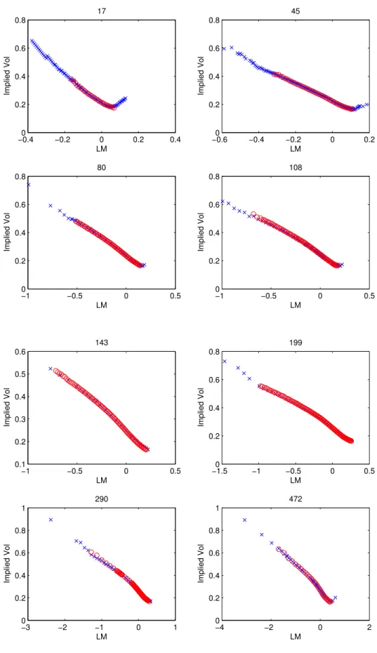
First, we look at the IVs for options on SPX and those on the ETF SPY. The implied volatilities are remarkably close: for September 1, 2010, we show the first eight maturities in Figure 2.
Next, we look at how implied volatilities on SPY and the −2x LETF SDS compare. On September 1, 2010, SDS has five maturities. Figure 4 shows the implied volatilities at each of the common maturities. Panel 4(f) shows the ratios of the implied volatilities (interpolating the SPY implied volatilities in LM to match them up). As the log-moneyness increases, the ratio increases from about 0.4 to around 1.8. Here the range is wider than between SPY and SSO. Again, the ratio is closest to 1 when the log-moneyness is slightly greater than zero (near-the-money).
Our first observation is that the implied volatilities from leveraged and unleveraged ETF options of the same log-moneyness and maturity are clearly not the same. The SSO IVs decrease with LM, have a shallower negative skew as compared with SPY, and cross near-the-money. On the other hand, SDS IVsincreasewith LM, as they are short in the S&P 500, and they also cross the SPY IV skew near the money. In addition, for both SSO:SPY and SDS:SPY ratios, they have an apparent structure of increasing as LM increases, being closest near-the-money.
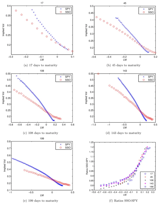
Next, we look at how implied volatilities on SPY and the 2x LETF SSO compare. On September 1, 2010, SSO has only five maturities, but generally strike prices over a broader range. Figure 3 shows the implied volatilities at each of the common maturities and the ratio of the implied volatilities (interpolating the SPY IVs in LM to match them up). In Figure 3(f), we illustrate the IV ratios between SSO and SPY options, for long and short maturities. As the log-moneyness increases, the ratio increases from about 0.8 to around 1.2. The ratio is closest to 1 when the
−0.40 −0.2 0 0.2 0.4 0.2 0.4 0.6 0.8 17 LM Implied Vol −0.60 −0.4 −0.2 0 0.2 0.2 0.4 0.6 0.8 45 LM Implied Vol −1 −0.5 0 0.5 0 0.2 0.4 0.6 0.8 80 LM Implied Vol −1 −0.5 0 0.5 0 0.2 0.4 0.6 0.8 108 LM Implied Vol −1 −0.5 0 0.5 0.1 0.2 0.3 0.4 0.5 0.6 143 LM Implied Vol −1.50 −1 −0.5 0 0.5 0.2 0.4 0.6 0.8 199 LM Implied Vol −3 −2 −1 0 1 0 0.2 0.4 0.6 0.8 1 290 LM Implied Vol −4 −2 0 2 0 0.2 0.4 0.6 0.8 1 472 LM Implied Vol
Figure 2: SPX (blue cross) and SPY (red circles) implied volatilities on September 1, 2010 for different maturities (from17to472 days) plotted against log-moneyness.
log-moneyness is slightly greater than zero (near-the-money).
3.2 Implied Volatility Comparison via Moneyness Scaling
The most salient features of the empirical implied volatilities in Figures 2-4 are: (i) the IV curve for SSO (β = 2) appears to be flatter than that for SPY (β = 1), and (ii) the IV curve for SDS (β =−2) is upward sloping as opposed to downward sloping like those for SPY (β = 1) and SSO (β = 2).
In order to explain these patterns, we introduce the idea of linking implied volatilities between ETF and LETF options via the method of moneyness scaling. This will be useful for traders to compare the option prices across not only different strikes but also different leverage ratios, and potentially identify option price discrepancies. One plausible explanation for the different IV patterns is that different leverage ratios correspond to different underlying dynamics. Therefore, the distribution of the terminal price of anyβ-LETF naturally depends on the leverage ratio β.
In a general stochastic volatility model, we can write the log LETF price as log LT L0 =βlog XT X0 −(r(β−1) +c)T −β(β−1) 2 Z T 0 σt2dt,
where (σt)t≥0 is the stochastic volatility process. The terms log LT L0 and log XT L0
are the log-moneyness of the terminal LETF value and terminal ETF value. Next, we condition on that the terminal (random) log-moneyness log
XT
X0
equal to some constant LM(1), and compute the conditional expectation of the β-LETF log-moneyness. This leads us to define
LM(β) :=βLM(1)−(r(β−1) +c)T− β(β−1) 2 IE ? Z T 0 σt2dt log XT X0 =LM(1) . (25)
In other words,LM(β)is the best estimate for the terminal log-moneyness ofL
T, given the terminal value logXT
X0
=LM(1). This equation strongly suggests a relationship between the log-moneyness between ETF and LETF options, though the conditional expectation in (25) is non-trivial.
In order to obtain a more explicit and useful relationship, let us consider the simple case with a constant σ as in the Black-Scholes model. Then, equation (25) reduces to
LM(β)=β LM(1)−(r(β−1) +c)T−β(β−1)
2 σ
2T. (26)
By this formula, theβ-LETF log-moneynessLM(β)is expressed as an affine function of the unlever-aged ETF log-moneyness LM(1). The leverage ratio β not only scales the log-moneyness LM(1), but also plays a role in two constant terms.
Interestingly, the moneyness scaling formula (26) can also be derived using the idea of Delta matching, as we show next.
Proposition 3 Under the Black-Scholes model, an ETF call option with log-moneynessLM(1) and a β-LETF call option with log-moneynessLM(β). The two calls have the same Delta if and only if (26) holds.
Proof. We equate the Deltas for the ETF and β-LETF calls:
LM(1)+ (r−σ2 2 )T
σ√T =
LM(β)+ (r−c−β22σ2)T
−0.3 −0.2 −0.1 0 0.1 0.2 0.25 0.3 0.35 0.4 17 LM Implied Vol SPY SSO
(a) 17 days to maturity
−0.6 −0.4 −0.2 0 0.2 0.2 0.25 0.3 0.35 0.4 0.45 0.5 45 LM Implied Vol SPY SSO (b) 45 days to maturity −0.8 −0.6 −0.4 −0.2 0 0.2 0.4 0.6 0.2 0.25 0.3 0.35 0.4 0.45 0.5 0.55 108 LM Implied Vol SPY SSO (c) 108 days to maturity −1.5 −1 −0.5 0 0.5 0.2 0.25 0.3 0.35 0.4 0.45 0.5 0.55 143 LM Implied Vol SPY SSO (d) 143 days to maturity −1 −0.5 0 0.5 0.1 0.2 0.3 0.4 0.5 0.6 0.7 0.8 199 LM Implied Vol SPY SSO
(e) 199 days to maturity
−0.8 −0.7 −0.6 −0.5 −0.4 −0.3 −0.2 −0.1 0 0.1 0.2 0.3 0.75 0.8 0.85 0.9 0.95 1 1.05 1.1 1.15 1.2 1.25 LM Ratios SSO:SPY 17 45 108 143 199 (f) Ratios SSO:SPY
Figure 3: SPY (blue cross) and SSO (red circles) implied volatilities against log-moneyness (LM) for in-creasing maturities. Panel (f ) shows SSO:SPY implied volatility ratios for different maturities.
−0.2 −0.1 0 0.1 0.2 0.3 0.2 0.25 0.3 0.35 0.4 17 LM Implied Vol SPY SDS
(a) 17 days to maturity
−0.4 −0.2 0 0.2 0.4 0.6 0.2 0.25 0.3 0.35 0.4 0.45 0.5 45 LM Implied Vol SPY SDS (b) 45 days to maturity −0.8 −0.6 −0.4 −0.2 0 0.2 0.4 0.6 0.2 0.25 0.3 0.35 0.4 0.45 0.5 0.55 108 LM Implied Vol SPY SDS (c) 108 days to maturity −1 −0.5 0 0.5 1 0.2 0.25 0.3 0.35 0.4 0.45 0.5 0.55 143 LM Implied Vol SPY SDS (d) 143 days to maturity −1 −0.8 −0.6 −0.4 −0.2 0 0.2 0.4 0.1 0.2 0.3 0.4 0.5 0.6 0.7 0.8 199 LM Implied Vol SPY SDS
(e) 199 days to maturity
−0.8 −0.7 −0.6 −0.5 −0.4 −0.3 −0.2 −0.1 0 0.1 0.2 0.3 0.4 0.6 0.8 1 1.2 1.4 1.6 1.8 2 LM Ratios SDS:SPY 17 45 108 143 199 (f) Ratios SDS:SPY
Figure 4: SPY (blue cross) and SDS (red circles) implied volatilities against log-moneyness (LM) for in-creasing maturities. Figure 4(f ) shows SDS:SPY implied volatility ratios for different maturities.
Rearranging both sides leads us to formula (26) connectingLM(1) andLM(β).
In the same spirit, we can apply (26) to link the log-moneyness pair (LM(β), LM( ˆβ)) of LETFs with different leverage ratios (β,βˆ), namely,
LM(β)= β ˆ β LM( ˆβ)+ (r( ˆβ−1) + ˆc)T +βˆ( ˆβ−1) 2 σ 2T −(r(β−1) +c)T −β(β−1) 2 σ 2T, (28)
where ˆc is the fee associated with the ˆβ-LETF.
In summary, the proposed moneyness scaling method is a simple and intuitive way to identify the appropriate pairing of ETF andβ-LETF IVs. In other words, for each β-LETF IV, the associated log-moneynessLM(β) can be viewed as a function of the log-moneynessLM(1) associated with the unleveraged ETF. Consequently, we can plot the IVs for both theβ-LETF and ETF over the same axis of log-moneyness LM(1) (see Figures 5 and 6). As a result, we can compare the LETF IVs with the ETF IVs by plotting them over the same log-moneyness axis. In practical calibration, we do not observe or assume a constant volatility σ. In order to apply moneyness scaling formula (26), we replace σ with the average IV across all available strikes for the ETF options. A more cumbersome alternative way is to estimate the conditional expectation of the integrated volatility in (25).
Let us first consider an example of mapping the IVs under the same mean-reverting stochastic volatility in (24) and Figure 1. In Figure 5, we show the IVs with the moneyness scaling for the LETFs withβ = 2 andβ = 3 in comparison with the IVs on the corresponding ETF. For each strike, expressed in terms of log-moneyness, of an LETF option, we apply (26) to get the corresponding log-moneyness of an ETF option. Compared to Figure 1, the three IV curves fit significantly better and their slopes are remarkably closer.
Next, we apply the log-moneyness scaling to the empirical IVs. In Figure 6, we plot both the ETF and LETF IVs after moneyness scaling on September 1, 2010 with 108 days to maturity. As we can see, the mapping works remarkably well as the LETF and ETF IVs overlap significantly, except in the SPXU case. In contrast to Figures 2-4, the IVS for the short LETFs, SDS and SPXU, are nowdownward sloping and are almost parallel with the SPY IVs. As a result, the log-moneyness scaling allows us to visibly discern the potential mismatch between ETF and LETF IVs.
4
Implied Volatility Asymptotics for LETF Options
In this section, we study LETF option implied volatilities within a multiscale stochastic volatility framework. An asymptotic approximation will allow us to examine the role played by the leverage ratioβ in a parsimonious fashion. Starting in the class of two-factor diffusion stochastic volatility models described by their characteristic time scales of fluctuation (one fast mean-reverting, one slowly varying), the implied volatility approximation allows us to trace how β impacts the level and skew structure, as well as the term-structure from LETF options, as compared to the unlever-aged ETF options. Just as implied volatility can be seen as a synoptic quantity that is useful in visualizing the departure of market options data from a constant volatility theory, the group parameters identified by the asymptotics provides a lens through which to analyze relationships between leveraged and unleveraged implied volatility surfaces.
−0.5 −0.4 −0.3 −0.2 −0.1 0 0.1 0.2 0.15 0.2 0.25 0.3 0.35 0.4 0.45 L o g - M o n e y n e s s I m p li e d V o la t il it y ETF LEFT (β=2) LEFT (β=3)
Figure 5: The IVs of call options on the ETF (cross), LETF with β = 2 (circle), and LETF with β = 3 (dot), plotted over the log-moneyness LM(1). In contrast to Figure 1, the three IV curves are now visibly closer.
Y and slow volatility factorZ are described by the system of SDEs:
dXt = rXtdt+f(Yt, Zt)XtdWt(0)? (29) dLt = (r−c)Ltdt+βf(Yt, Zt)LtdWt(0)? (30) dYt = 1 εα(Yt)− 1 √ εη(Yt)Λ1(Yt, Zt) dt+√1 εη(Yt)dW (1)? t (31) dZt = δ `(Zt)−√δ g(Zt)Λ2(Yt, Zt) dt+ √ δ g(Zt)dWt(2)?. (32)
Here, the standard IP?-Brownian motions W(0)?, W(1)?, W(2)? are correlated as follows:
dhW(0)?, W(1)?it=ρ1dt, dhW(0)?, W(2)?it=ρ2dt, dhW(1)?, W(2)?it=ρ12dt ,
where|ρ1|, ρ2|,|ρ12|<1, and 1 + 2ρ1ρ2ρ12−ρ21−ρ22−ρ212>0, in order to ensure positive definiteness of the associated covariance matrix. The correlation coefficients capture skew effects that are an important feature of typical implied volatility surfaces. Under the pricing measure IP?, Λ1(y, z) and Λ2(y, z) are the associated market prices of volatility risk. The dynamics of Y and Z under the historical measure IP are given by setting Λ1 and Λ2 to zero in (31) and (32) (and replacing the Brownian motions by IP-Brownian motions).
The small positive parameter εcorresponds to the short mean-reversion time scale of the fast volatility factorY. The coefficientsα(y) andη(y) need not be specified for our asymptotic analysis, as long as the corresponding process Y is mean-reverting (ergodic) under IP, and has a unique invariant distribution denoted by Φ that is independent ofε. We assume that the volatility function
f is positive, smooth inz, and such thatf2(·, z) is integrable with respect to Φ. While specifyingε
is not needed here (it will be contained in terms calibrated from data), one typically thinks of this fast factor as capturing mean-reversion in volatility on the scale of a few days.
On the other hand, the small positive parameter δ characterizes the slow volatility factor Z. The coefficients `(z) and g(z) need not be specified for our analysis. Againδ does not need to be
−0.8 −0.6 −0.4 −0.2 0 0.2 0.2 0.25 0.3 0.35 0.4 0.45 0.5 0.55 108 LM Implied Vol SPY SSO (a) SSO −0.8 −0.6 −0.4 −0.2 0 0.2 0.2 0.25 0.3 0.35 0.4 0.45 0.5 0.55 108 LM Implied Vol SPY SDS (b) SDS −0.8 −0.6 −0.4 −0.2 0 0.2 0.2 0.25 0.3 0.35 0.4 0.45 0.5 0.55 108 LM Implied Vol SPY UPRO (c) UPRO −0.8 −0.6 −0.4 −0.2 0 0.2 0.2 0.25 0.3 0.35 0.4 0.45 0.5 0.55 108 LM Implied Vol SPY SPXU (d) SPXU
Figure 6: SPY (blue cross) and LETF (red circles) implied volatilities after moneyness scaling on September 1, 2010 with 108 days to maturity, plotted against log-moneyness of SPY options.
specified at this stage (it will appear in parameters calibrated from data), but one may think of the slow factor as describing volatility fluctuations on a time scale of a few months.
This class of models has been applied to price equity options (that is, on X) in Fouque et al. (2011), where further technical details and empirical motivation are provided. Next, we investigate the impact of leverageβ on the pricing of LETF options and their implied volatilities.
4.1 Options on Index or Unleveraged ETF
We first consider the pricing of a European option onXand its implied volatility. The no arbitrage price of a European option with terminal payoffh(XT), representing either a call or put option, is given by Pε,δ(t, Xt, Yt, Zt) = IE? n e−r(T−t)h(XT)|Xt, Yt, Zt o .
The function Pε,δ(t, x, y, z) solves a high-dimensional partial differential equation. This is very computationally intensive to solve and does not lead to efficient calibration procedures.
Alterna-tively, we apply the perturbation theory, as discussed in Fouque et al. (2011), in order to simplify the calibration problem and shed light on the implied volatilities.
We summarize the main steps. In the following, we denote byh·i averaging with respect to the invariant distribution Φ. We define:
1. The averaged effective volatility σ¯(z) is defined by
¯
σ2(z) =hf2(·, z)i=
Z
f2(y, z)Φ(dy). (33)
2. The corrected volatility parameterσ?(z) is composed of ¯σ adjusted by a small term from the market price of volatility risk from the fast factorY:
σ?(z) =
q
¯
σ2(z) + 2Vε
2(z), (34)
whereV2ε(z) is of order√εand is given by
V2ε(z) = √ ε 2 ηΛ1 ∂φ ∂y . (35)
Here φ(y, z) is a solution to the Poisson equation: 1 2η 2(y)∂2φ ∂y2 +α(y) ∂φ ∂y =f 2(y, z)−σ¯2(z). (36)
Note thatφis defined up to an arbitrary additive function of z, but this will play no role in the approximation below.
3. The three group parameters: V3ε containing the correlation ρ1 between shocks to the fast factor Y and shocks to the index X is given by
V3ε(z) =−ρ1 √ ε 2 ηf∂φ ∂y . (37)
It is of order √ε. Next, V0δ contains the market price of volatility risk from the slow factor
Z: V0δ(z) =−g(z) √ δ 2 Λ2 ¯ σ0(z), (38)
and V1δ contains the correlation ρ2 between shocks to the slow factor Z and shocks to the indexX V1δ(z) = ρ2g(z) √ δ 2 fσ¯0(z), (39)
and bothV0δ and V1δ are of order √δ.
Proposition 4 For fixed (t, x, y, z), the European option price Pε,δ(t, x, y, z) is approximated by
P?(t, x, z), where P? =PBS? + τ V0δ+τ V1δ x ∂ ∂x +V ε 3 σ? x ∂ ∂x ∂PBS? ∂σ , (40)
and the order of accuracy is given by
Pε,δ=P?+O(εlog|ε|+δ). (41) Here,PBS? is the Black-Scholes call price with time-to-maturityτ =T−tand the corrected volatility parameter σ?.
We refer to (Fouque et al., 2011, Chapters 4-5) for the derivation and accuracy proof of these formulas. Note that the stochastic volatility correction terms in (40) are comprised of Greeks of the Black-Scholes pricePBS? , in particular the Vega and the Delta-Vega.
In order to compute this approximated priceP?, only thegroup market parameters(σ?, V0δ, V1δ, V3ε) need to be estimated from the term structure of implied volatilities obtained from European call and put options. The price approximation (40) can be used to derive the implied volatility I as-sociated with Pε,δ defined by PBS(I) = Pε,δ. To do so, we define the variable Log-Moneyness to Maturity Ratioby
LMMR = log(K/x)
τ . (42)
Proposition 5 The first-order approximation for the implied volatility is given by
I =b?+τ bδ+aε+τ aδLMMR+O(εlog|ε|+δ), (43)
where the parameters (b?, bδ, aε, aδ) are defined in terms of (σ?, V0δ, V1δ, V3ε) by
b?=σ?+ V ε 3 2σ? 1− 2r σ?2 , aε= V ε 3 σ?3, bδ=V0δ+V δ 1 2 1− 2r σ?2 , aδ= V δ 1 σ?2.
We refer to (Fouque et al., 2011, Section 5.1) for the derivation of these formulas. Note that V3ε
is of order √ε whereas Vδ
0 and V1δ are both of order √
δ. The implied volatility approximation shows that the interceptb? is of order one, the slope coefficientsaε andaδ are of order√εand√δ
respectively, and that bδ is of order √δ.
4.2 Options on Leveraged ETF
We now proceed to investigate the role of β in the coefficients and parameters in the first-order approximation of LETF option prices. First, the risk-neutral price of a European LETF option with terminal payoffh(LT) is given by
Pβε,δ(t, Lt, Yt, Zt) = IE?
n
e−r(T−t)h(LT)|Lt, Yt, Zt
o
.
The main goal is to trace how theβ introduced in the scaling of the volatility term in (30) enters the various parts of the asymptotics. For simplicity, we assume the expense feec= 0.
Proposition 6 For fixed (t, x, y, z), the LETF option price Pβε,δ(t, x, y, z) is approximated by
Pβε,δ=Pβ?+O(εlog|ε|+δ), where Pβ? =PBS?,β+ ( τ V0δ,β+τ V1δ,β x ∂ ∂x + V ε 3,β σβ? x ∂ ∂x ) ∂PBS?,β ∂σ .
Here the β-dependent group market parameters are:
V0δ,β =|β|V0δ, V1δ,β =β|β|V1δ, V3ε,β =β3V3ε, σβ? =|β|σ?, (44)
and PBS?,β is the Black-Scholes call option price with time-to-maturity τ =T −t and the corrected volatility parameter σ?β.
Proof. These follow from repeating Proposition 4 with f replaced by βf. Indeed we have the following replacements: from (33), ¯σ2 7→ β2σ¯2 and so ¯σ 7→ |β|σ¯; from (36), φ7→ β2φ; from (35),
V2ε 7→ β2V2ε, and so from (34), σ? 7→ |β|σ?; from (37), V3ε 7→ β3V3ε; from (38), V0δ 7→ |β|V0δ; and finally from (39),V1δ7→β|β|V1δ.
Note thatβ enters the group parameters in different ways rather than just simply scaling them. The next goal is to see howβimpacts the calibration parameters that are fit to the implied volatility surface.
Proposition 7 The implied volatility of an LETF option I(β) is defined as in (7)by
I(β) = 1 |β|P
−1 BS(Pβ),
where the inversion of the Black-Scholes formula is with respect to volatility. Its first-order approx-imation, to order of accuracy O(εlog|ε|+δ), is
I(β) ≈ b?β+τ bδβ +
aεβ+τ aδβ
LMMR, (45)
where the skew slopes are given in terms of the unleveraged ETF skew slopes by
aεβ = 1 βa ε, aδ β = 1 βa δ, (46)
and where the level parameters(b?β, bδβ)are given in terms of the unleveraged ETF group parameters (σ?, V0δ, V1δ, V3ε) by b?β =σ?+βV ε 3 2σ? 1− 2r β2σ?2 , bδβ =V0δ+ βV δ 1 2 1− 2r β2σ?2 . (47)
Proof. From Proposition 5, the approximation for |β|I(β) is given by
|β|I(β)≈bb?β+τbbδ β+ c aεβ+τcaδ β LMMR,
whereLM M R= log(K/Lt)/τ is defined w.r.t. the LETF spot price Lt, and
b b? β =σ ? β+ V3ε,β 2σβ? 1− 2r σ?β2 ! , acεβ = V3ε,β σβ?3, b bδ β =V δ 0,β+ V1δ,β 2 1− 2r σ?β2 ! , acδ β = V1δ,β σβ?2.
Substituting from (44) and dividing by |β|leads to (45) and the relations (46)-(47).
We note first that the first-order approximation reveals that the skew slope parameters have the direct relationship (46), and so in particular the short leveraged ETFs implied volatilities have the opposite signed slopes as we saw in Figure 4 for β =−2. The relationship between the level parameters (theb’s) is not direct, but is given in (47) after passing through theV’s. These relations can be used to assess how less liquid LETF implied volatility surfaces relate to the more liquid ETF IV surface within the framework of multiscale stochastic volatility, and we look at data in the next section.
5
Analysis of ETF & LETF Implied Volatility Surfaces
Proposition 7 suggests a link between the approximated IVs of an ETF and its leveraged coun-terparts. Hence, one can first calibrate the stochastic volatility group parameters using unlever-aged ETF option data, such as those on SPY. This will give the estimated group parameters (σ?, V0δ, V1δ, V2ε, V3ε). Then, we use (46) and (47) to get the approximated LETF options implied volatility (45).
This procedure is useful in practice especially when the index/ETF option data is significantly richer than the LETF option data. Indeed, the unleveraged market typically has better liquidity and more contracts with different strikes and maturities traded. On the other hand, one can directly use the LETF option data to calibrate the approximated IVs. We shall compare the two approaches to better understand the IVs of LETF options.
5.1 From SPY IVs to LETF IVs
We first apply our IV approximation using option data from SPY to four associated leveraged ETFs, namely, SSO, SDS, UPRO, and SPXU. Approximation (43) is fitted to the SPY IV surface to obtain least-squares estimates of (aε, b?, aδ, bδ) which give predictions for (aεβ, b?β, aδβ, bδβ) via (46) and (47).
In Figure 7, we overlay the IVs of LETF options from August 23, 2010 with the IV approx-imation based on SPY option data. The LETF options shown have 117 days to maturity. The calibration that leads to the predicted approximation involves using SPY options data of all avail-able maturities. Figure 8 shows the data and predictions for 208-day maturity LETF options. In general, we observe that the predicted slope is reasonably close, except in the one case in panel 8(b) where the data looks atypically flat. This suggests that the β-effect on the correlation or skew is quite consistent between theory and data. On the other hand, there seems to be greater mismatch in the IV level between data and the prediction. Since, in the theory, this is related through the b’s (see (47)) to the market prices of volatility risk, it suggests differing risk premia across the different products.
Next, we examine the difference between prediction from SPY calibration and LETF option data by repeating this procedure every day from September 1st 2009 to September 1st 2010. In Figure 9, we show the relative errors in the predicted slopes and intercepts compared with a direct least-squares fit to each LETF IV skew for each maturity. Note that the prediction uses data from all maturities from one product, namely SPY, and its performance is measured against a direct affine fit to a single maturity skew on another product. The mean and standard deviation of the relative errors are reported in Table 1. From these, we see that the slope errors are negatively
SSO SDS UPRO SPXU
Intercept Relative Error mean 0.13% -0.07% 1.41% 7.49%
std dev. 2.36% 3.36% 4.83% 20.60%
Slope Relative Error mean -15.51% 15.04% -20.00% -3.76%
std dev. 8.94% 42.55% 9.51% 6.74%
Table 1: The relative errors of the SPY-predicted intercept and slope for the IVs for SSO, SDS, UPRO, and SPXU, over the period September 2009 to September 2010.
−0.8 −0.6 −0.4 −0.2 0 0.2 0.4 0.6 0.2 0.25 0.3 0.35 0.4 0.45 0.5 117 LM Implied Vol SSO Prediction (a) SSO −0.4 −0.2 0 0.2 0.4 0.6 0.18 0.2 0.22 0.24 0.26 0.28 0.3 0.32 0.34 0.36 0.38 117 LM Implied Vol SDS Prediction (b) SDS −0.8 −0.6 −0.4 −0.2 0 0.2 0.4 0.6 0.16 0.18 0.2 0.22 0.24 0.26 0.28 0.3 0.32 0.34 0.36 117 LM Implied Vol UPRO Prediction (c) UPRO −0.8 −0.6 −0.4 −0.2 0 0.2 0.4 0.6 0.18 0.2 0.22 0.24 0.26 0.28 0.3 0.32 0.34 0.36 117 LM Implied Vol SPXU Prediction (d) SPXU
Figure 7: IVs of LETF options with 117 days to maturity and prediction from SPY calibration.
order of magnitude than those for the other LETFs). For the intercept, the±2 LETFs have better consistency with SPY than the more leveraged±3 LETFs where the risk premium mismatch seems greater.
−0.8 −0.6 −0.4 −0.2 0 0.2 0.4 0.6 0.18 0.2 0.22 0.24 0.26 0.28 0.3 0.32 0.34 0.36 0.38 208 LM Implied Vol SSO Prediction (a) SSO −0.6 −0.4 −0.2 0 0.2 0.4 0.18 0.2 0.22 0.24 0.26 0.28 0.3 0.32 0.34 208 LM Implied Vol SDS Prediction (b) SDS −0.8 −0.6 −0.4 −0.2 0 0.2 0.4 0.6 0.18 0.2 0.22 0.24 0.26 0.28 0.3 0.32 0.34 208 LM Implied Vol UPRO Prediction (c) UPRO −0.8 −0.6 −0.4 −0.2 0 0.2 0.4 0.6 0.2 0.22 0.24 0.26 0.28 0.3 0.32 208 LM Implied Vol SPXU Prediction (d) SPXU
−0.40 −0.2 0 0.2 0.4 10
20 30
SSO Slope Relative Error
−0.10 −0.05 0 0.05 0.1
10 20 30
SSO Intercept Relative Error
−1 0 1 2 3 0 20 40 60 80
SDS Slope Relative Error
−0.10 −0.05 0 0.05 0.1 0.15
10 20 30 40
SDS Intercept Relative Error
−0.60 −0.4 −0.2 0 0.2
10 20 30 40
UPRO Slope Relative Error
−0.20 −0.1 0 0.1 0.2
10 20 30
UPRO Intercept Relative Error
−0.50 0 0.5 1 1.5
20 40 60 80
SPXU Slope Relative Error
−0.10 0 0.1 0.2 0.3 0.4
10 20 30 40
SPXU Intercept Relative Error
Figure 9: Histogram of relative errors of SPY-calibrated predictions of the IV slopes and intercepts for SSO, SDS, UPRO, SPXU, collected over the period September 2009 to September 2010.
5.2 Direct Fitting to LETF IV Surfaces
Now we fit the implied volatility approximation in Proposition 7, formula (45) directly to LETF IV data across all maturities. These are shown for August 23, 2010 in Figure 10. As there are fewer traded contracts to fit, the fits are typically better than for the SPY, and are reasonably good. This suggests multiscale stochastic volatility is a decent approximation for LETF IVs in their own right. −8 −6 −4 −2 0 2 4 0.2 0.25 0.3 0.35 0.4 0.45 0.5 0.55 LMMR Implied Volatility
Fitted Surface and Data −− SSO
(a) SSO −4 −3 −2 −1 0 1 2 3 4 5 6 0.18 0.2 0.22 0.24 0.26 0.28 0.3 0.32 0.34 0.36 LMMR Implied Volatility
Fitted Surface and Data −− SDS
(b) SDS −10 −8 −6 −4 −2 0 2 4 0.2 0.25 0.3 0.35 0.4 LMMR Implied Volatility
Fitted Surface and Data −− UPRO
(c) UPRO −4 −3 −2 −1 0 1 2 3 4 5 6 0.18 0.2 0.22 0.24 0.26 0.28 0.3 0.32 LMMR Implied Volatility
Fitted Surface and Data −− SPXU
(d) SPXU
Figure 10: LETF options IVs and their calibrated first-order approximations for all available maturities on August 23, 2010.
Next, we consider how the empirical skew slopes respect the relations (46). To do so, we calibrate daily the skew parameters (aεβ, aδβ) for β ∈ {1,±2,±3}. Then we fix an arbitrary mid-range maturity,τ = 100 days, and look at the ratios
Rij := aεβ i+τ a δ βi aεβ j+τ a δ βj , i, j ∈ {1,±2,±3}, i6=j,
for the 10 pairwise combinations. In theory, we should have
Of course this does not hold so cleanly in the data, and we are interested in any systematic deviation from these relationships. Since it is not clear which data might be “preferentially correct”, we give the five datasets equal weighting and calculate estimates of each βi as ifβj were correct, and then average over the four estimates for each βi.
That is, for each daily observation Rij, we can compute estimated
b
βj|i:=βiRij, βbi|j :=βj/Rij.
The histograms of the daily averaged estimates ¯ βi = 1 4 X j6=i b βi|j
are presented in Figure 11, and the means and standard deviations are in Table 2. These results
0 100 200 300 0.8 1 1.2 1.4 Day number Daily implied β 1 for SPY 0.8 1 1.2 1.4 0 5 10 15 Implied SPY β 1 1.4 1.6 1.8 2 2.2 2.4 2.6 2.8 0 5 10 15 20 Implied SSO β 2 −4.50 −4 −3.5 −3 −2.5 −2 −1.5 10 20 30 Implied SDS β −2 1.8 2 2.2 2.4 2.6 2.8 3 0 5 10 15 Implied UPRO β 3 −5 −4.5 −4 −3.5 −3 −2.5 0 10 20 30 40 50 Implied SPXU β −3
Figure 11: Histograms ofβ¯i, the impliedβ from September 2009-September 2010 LETF implied volatilities.
SPY SSO SDS UPRO SPXU ¯
β mean 1.0512 1.9840 -2.6314 2.4705 -2.9264
¯
β standard dev. 0.1092 0.1596 0.5101 0.2605 0.4780
Table 2: The mean and standard deviation of estimated β¯ over September 2009-September 2010 for SPY, SSO, SDS, UPRO, and SPXU.
leverage ratios of 1,2 and −3 respectively. However implied volatility skews from SDS (β = −2) systematicallyoverestimatethe magnitude of leverage ratio, as if the LETF was more short than it is actually supposed to be. In contrast the skews from UPRO (β= 3) systematicallyunderestimate the leverage ratio, as if the LETF was not so ultra-leveraged. While these are findings are dependent on our framework for analyzing the data, the systematic discrepancies are very striking.
6
Conclusion
The recent growth of leveraged ETFs and their options markets calls for research to understand the inter-connectedness of these markets. In our study, we have investigated from both empirical and theoretical perspectives implied volatilities of options on LETFs with different leverage ratios. Our analytical results have led us to examine implies volatilities in several ways. First, we propose the method of moneyness scaling to enhance the comparison of IVs with different leverage ratios. Then, under the multiscale stochastic volatility framework, we use unleveraged ETF option data to calibrate for the necessary parameters to arrive at a predicted LETF options implied volatility ap-proximation (see Proposition 7). This approach allows us to use the richer unleveraged index/ETF option data to shed light on the less liquid LETF options market. Alternatively, we also calibrate directly from LETF option data to obtain the approximated implied volatilities.
Our calibration examples confirm the approximate connection between ETF and LETF IVs, while volatility risk premium may differ across LETF options markets, especially for the double-short and triple-double-short LETFs. Of course, it will be of future interest to perform the analogous analy-sis in other regimes that have been studied in the unleveraged case: large strike (Lee (2004); Gulisas-hvili and Stein (2009)); long maturity (Tehranchi (2009)); or short time-to-expiration (Berestycki et al. (2004)).
Leveraged exchange-traded products are also available for other reference indexes such as Nas-daq 100 and Russell 2000, as well as other asset classes such as commodities and real estate. For volatility trading, there are the S&P 500 Short-Term VIX Futures Index ETN (VXX), and Mid-Term VIX Futures Index ETN (VXZ), as well as options on these two ETNs traded on CBOE. All these should motivate research to investigate the connection between derivatives prices and the consistency thereof. In this regard, models that are tractable and capable of capturing the characteristics of inter-connected markets are highly desirable. A related issue is to quantify the leverage risks and the feedback effect on market volatility created by ETFs and LETFs1, not to mention what might occur if a sizeable LETF option market is not well studied and understood. Acknowledgements
We thank Andrew Ledvina for initial research assistance with the data, and Marin Nitzov for bringing the problem to our attention.
References
Ahn, A., Haugh, M., and Jain, A. (2012). Consistent pricing of options on leveraged ETFs. working paper, Columbia University.
Avellaneda, M. and Zhang, S. (2010). Path-dependence of leveraged ETF returns. SIAM Journal of Financial Mathematics, 1:586–603.
Bayraktar, E. (2008). Pricing options on defaultable stocks. Applied Mathematical Finance, 15(3):277–304.
Berestycki, H., Busca, J., and Florent, I. (2004). Computing the implied volatility in stochastic volatility models. Comm. Pure Appl. Math., 57(10):1352–1373.
Cheng, M. and Madhavan, A. (2009). The dynamics of leveraged and inverse exchange traded funds. SSRN.
Cotton, P., Fouque, J., Papanicolaou, G., and Sircar, R. (2004). Stochastic volatility corrections for interest rate derivatives. Mathematical Finance, 14:173200.
Fouque, J.-P., Papanicolaou, G., Sircar, R., and Sølna, K. (2011). Multiscale Stochastic Volatility for Equity, Interest Rate, and Credit Derivatives. Cambridge University Press.
Gulisashvili, A. and Stein, E. (2009). Implied volatility in the Hull-White model. Mathematical Finance, 19:303–327.
Haugh, M. (2011). A note on constant proportion trading strategies. Operations Research Letters, 39:172–179.
Jaimungal, S. and Hikspoors, S. (2008). Asymptotic pricing of commodity derivatives for stochastic volatility spot models. Applied Mathematical Finance, 15(5-6):449–447.
Lee, R. (2004). The moment formula for implied volatility at extreme strikes.Mathematical Finance, 14(3):469–480.
Romano, M. and Touzi, N. (1997). Contingent claims and market completeness in a stochastic volatility model. Mathematical Finance, 7(4):399–410.
Russell, M. (2009). Long-term performance and option pricing of leveraged ETFs. Senior Thesis, Princeton University.
Tehranchi, M. (2009). Asymptotics of implied volatility far from maturity. Journal of Applied Probability, 46:629–650.
Zhang, J. (2010). Path dependence properties of leveraged exchange-traded funds: compounding, volatility and option pricing. PhD thesis, New York University.