On the Use of the First Principal Component as a Core Inflation Indicator

BANCO DE PORTUGAL Economic Research Department

ON THE USE OF THE FIRST

PRINCIPAL COMPONENT AS ACORE

INFLATION INDICATOR

José Ramos Maria

WP 3-04 January 2004

The analyses, opinions and findings of these papers represent the views of the authors, they are not necessarily those of the Banco de Portugal.

Please address correspondence to José Ramos Maria, Economic Research Department, Banco de Portugal, Av. Almirante Reis nº. 71, 1150-165 Lisboa, Portugal;

On the use of the first principal component

as a

core

inflation indicator

Jos´e Ramos Maria∗

Banco de Portugal January 2004

Abstract

This paper investigates if the (OLS-scaled) first principal component (P C₁), extracted from standardized yearly rates of change of basic items of the CPI, represents a reasonable option for acoreinflation indicator. The evaluation is carried out by (i) confronting alternative linear transformations of the original variables; (ii) analyzing the impact of stacking lagged variables to the original database; and (iii) exploring the contents of the remaining principal components. An orthogonal factor model framework will also be introduced so as to fully reproduce any variable that can be expressed as a linear combination of the original input variables, such as, in this case, the overall inflation rate. The model incorporates the following properties: (i) the results are not conditional on the eigenvectors length; (ii) the variance of the CPI accounted for by each component is unique, and (iii) the outcome is equivalent to an OLS regression between the CPI and theP C1. Along with empirical evidence for the Portuguese case, it will be claimed that the above-mentioned (OLS-scaled)P C₁ does capture the general movement of the overall inflation rate, however, no OLS regression would have to be implemented if the core indicator is fully aligned with the orthogonal factor model.

KEYWORDS:Principal components, factor models, core inflation indicators.

JEL Classification: C43, E31.

Acknowledgements: I am indebted to Francisco Dias and to Maximiano Pinheiro for helpful comments and suggestions. The assistance of Teresa Nascimento was also appreciated. The usual disclaimer applies.

1

Introduction

Principal components analysis continues on being one of the most used techniques in multivariate analysis. Within the price development dimension, several authors have used this technique to estimate “summary indicators” and to classify those time series as trend inflation indicators. Recent work for the euro area includes, for instance,

Angelini, Henry and Mestre (2001_b), who use a time domain approach to estimate

a non-stationary factor that intends to represent a common trend in the inflation measures (along the lines suggested by Stock and Watson (1998); the forecasting

performance was address in Angelini, Henry and Mestre (2001_a)); and Cristadoro,

Forni, Reichlin and Veronese (2001), who use a frequency domain approach to extract a medium and long-run common component for consumer prices. Recent work with Portuguese data includes, for instance, Machado, Marques, Neves and Silva (2001).

This paper investigates if the (OLS-scaled) first principal component (P C1), extracted

in the time domain from standardized yearly rates of change of basic items of the

con-sumer price index (CP I), represents a reasonable option for a_core inflation indicator.

Currently, the Banco de Portugal uses this procedure to measure (and regularly

pub-lish) a_core inflation indicator for the Portuguese case. An objective of this paper is to

evaluate this option, which was proposed by Coimbra and Neves (1997), while look-ing for possible improvements. Machado et al. (2001) suggested, for instance, that to take into account the non-stationarity feature of the input variables, a specific linear transformation could be implemented, instead of making use of standardized

vari-ables, as in Coimbra and Neves. In both studies, the _core indicator is only derived

from the information contained in the basic _items of the Portuguese CP I, which

are mostly non-stationary data. Not surprisingly, the need of having to compare the

core measure with some observable variable raised the question of having to find an

“appropriate scaling” for the P C_i. In what has been classified as just an _“ad-hoc”

procedure, both studies solved this issue by running an OLS regression between the

inflation rate and the P C1 (and, therefore, depend on this final parameter to scale

the P C1). It will be shown that this decision has some important implications. The

current paper confronts the results obtained by these studies and, furthermore, in-vestigates if alternative linear transformations of the observed variables, within the same course of action, produce structurally different outcomes. It will be claimed

that none of the transformations have an obvious superiority or advantage; nor can the non-stationarity nature of the data be used to distinguished the overall results. Other possibilities of improvement, such as (i) stacking lagged variables to the original database, along the lines suggested for instance by Stock and Watson (1998) or (ii)

including more principal components for the derivation of the _core inflation indicator

are also analyzed.

The rest of the paper is organized as follows. Section 2 confronts the results obtained from alternative linear transformations of the original data. Section 3 analyzes the use of lagged variables in the database. The use of more than the first principal component is considered in section 4. Finally, section 5 introduces a simple theoretical orthogonal factor model that captures the general underlying conceptual framework

of the proposed indicator. The factor model fully reproduces the overall CP I, and

embodies several appealing properties, in which the so called_“ad-hoc” procedure has

a well defined interpretation. Without any assumption on the data generation process of the different input variables, it will be shown that the model represents a solution for the fundamental eigenvectors length indeterminacy, it uniquely determines the

variance of the CP I accounted for by each P C_i and it is fully equivalent to an OLS

regression, using the CP I as the endogenous variable and theP C_i as the exogenous

variables.

Section 6 concludes. It will be claimed that unless a smoother core inflation indicator

is being envisaged on _{a priori} grounds, no obvious gain seems to be achieved by

changing the currently used procedure at the Banco de Portugal. However, no OLS regression would have to be implemented if the core inflation indicator is fully aligned with the factor model introduced in section 5.

2

On the use of transformed variables

Let the matrix X be the initial information set, with N observable variables x1, x2,

..., x_N (in columns), andT observations (in lines). The principal components are just

special linear combinations of those initial variables and if none of the N variables is

an exact linear combination of the others, then there will exist as many distinct P C_i

as variables.

of the initial information set and therefore a decision has always to be made on whether the database justifies certain transformations prior to the calculation of the

P C.1 _{Given that the second moment matrix may be non-centered, the first common}

transformation of the original data is to subtract the mean of eachx_i. If one does not

wish to have a P C1 dominated by those variables who have the largest variance, then

a second common transformation is standardization and instead of deriving theP C1

from the variance-covariance structure of X (from now on denoted as Σ_X), the P C1

can be derived from the correlation matrix (from now on denoted asρ_X). Using

year-on-year rates of change of basic items of the CPI, which are basically non-stationary data, this was the procedure followed by Coimbra and Neves (1997). Let this linear transformation be denoted as LT1.

The general conceptual framework of Coimbra and Neves (1997) can be written down as    x1 =x₁ +l∗₁₁F₁∗+ε1 ... xN =xN +l1N∗ F1∗+εN (1)

wherex1,x2, ...,xN correspond to the average values ofx1t,x2t, ...,xNt;F1∗ represents

a common factor to all variables and F₁∗ =P C1; l∗1j =aj1, j = 1...N, where aj1

rep-resents the scalars defining the eigenvector (scaled to unity) associated to the largest

eigenvalue (extracted fromρ_X); and, finally,ε1, ε2, ...εN correspond to specific factors

of each variable. Note that the N variablesx1,..., xN are just being linearly expressed

in terms of their mean plus (1 +N) unobservable variables: F₁∗ and ε1, ε2, ...εN.2

Presumably, the behaviour of each year-on-year rate of change is not only reflecting specific factors but also the “inflation trend”.

It is well known that if the original variables are subject to LT1, the eigenvalues and resulting eigenvectors are in general not the same as the ones derived from

Σ_X, or even a simple function of them.3 _{If the eigenvectors are collected in A =}

a1 a2 ... aN

, this implies that, in general, the matrix A will depend on the

transformation.

Other transformations of the original (centered) variables are also available. For

1_{See Jackson (1991) and Jollife (2002).}

2_{This model is usually expressed in terms of deviations, i.e. (xi−xi), and to satisfy the usual assumption of}

unit variances of the common factors, theF_i should have been defined asF_i=P C_i/(V ar[P C_i]1/2) and, therefore, Fi=P C_i/√λ_i⇔P C_i=√λ_iF_i, withl_ij=√λ_ia_ji, instead of assumingP C_i=F_i∗. See, for instance, Afifi (1984).

instance, Machado et al. (2001) suggested that to take into account the non-stationary

feature of the original variables, the x_i should be scaled by (σ∆x_i)−1, where σ∆x_i

represents the standard error of the first difference of x_i. By defining the smoothness

of the integrated variable as the variance of the first differences, Machado et al. (2001) argue that a core inflation indicator should take into account the degree of smoothness

of the P C1 by looking at linear combinations of the year-on-year rates of change of

the basic CPI items “with a large signal (variance) and not to much volatility” (_p.7).

Let this linear transformation be denoted as LT2. Note that both possibilities can

be represented by a diagonal matrix H, with h_ii in the main diagonal, i = 1, ..., N,

where H is alternatively associated with LT1 or LT2, i.e.,

P C = (X−X)H−1A (2)

The principal components (extracted from unit length eigenvectors) are being

gath-ered in a matrix named P C, where the first principal component (P C1) is placed

in the first column of P C, the P C2 in the second, etc; and X corresponds to the

average values of x1t, x2t, ..., xNt. If hii = σi in (2), H is associated with LT1. If

hii = σ∆xi, and σ∆xi is the standard error of the first difference of xi, then H is

associated with LT2.4 This section will directly confront the results obtained

un-der this two transformations. However, other transformations (purely arbitrary and motivated by no reason, except for comparison purposes against LT1 or LT2) will also be implemented. Alternative linear transformations of the same type of LT1 or

LT2 may be given, for instance, by h_ii = [max(x_i)−min(x_i)], abbreviated to LT3;

or simply h_ii = max(x_i), abbreviated to LT4. Note that for each possibility, the

importance of each original (centered) variable (x_i −x) is just being changed by a

scaling constanth_ii−1, in particular when computing the second moment matrix from

which the scalars of the eigenvectors are extracted. In the case of LT1, for instance, the importance of the variables with high standard deviations will be highly affected

and the same follows for a higher σ∆x_i,[max(xi)−min(xi)] or max(xi) in the case of

LT2, LT3 or LT4, respectively.5

After having decided the relevant second moment matrix from which the matrix A

is derived, there is still the need to find comparable scores to those of the observed

4_{This type of representation by no means intends to express the entire group of transformations that the original}

variables may be subjected to. On this issue, see, for instance, Jollife (2002).

5_{A more elaborated transformation could be given byhii=σ}

∆2_xi, where ∆2x_irepresents the second difference of xi. However, the results from this transformation will not be reported, as they do not change the overall conclusions.

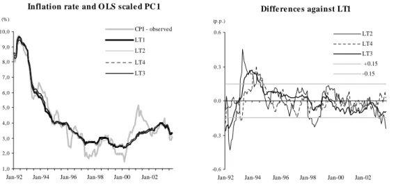
1,0 2,0 3,0 4,0 5,0 6,0 7,0 8,0 9,0 10,0

Jan-92 Jan-94 Jan-96 Jan-98 Jan-00 Jan-02 CPI - observed LT1 LT2 LT4 LT3

Inflation rate and O LS scale d PC 1

(%) -0.6 -0.3 0.0 0.3 0.6

Jan-92 Jan-94 Jan-96 Jan-98 Jan-00 Jan-02 LT2 LT4 LT3 +0.15 -0.15

Diffe re nce s against LT1

(p.p.)

Figure 1 - OLS results using the full sample period

overall inflation rate. To such purpose, Coimbra and Neves (1997) or Machado et al. (2001) computed the OLS fitted values of the following regression

·

CP I =β0+β1P C1+ε (3)

where CP I· denotes the observed inflation rate.

The database used by Coimbra and Neves (1997) and by Machado et al. (2001) has

90 variables (N = 90), with monthly year-on-year rates of change of basic _items of

the CP I. Following the EUROSTAT classification, 14 of those variables refer to

unprocessed food_items, 24 are processed food _items, 3 are energy _items, 26 are

non-energy industrial goods _items and 23 are services _items.6 _{The current paper makes}

use of 141 observations, covering the period 1992:01-2003:09, and the same proce-dures will be extended to the other loosely defined transformations (LT3 and LT4). Therefore, the principal components methodology will be just used as a mechanical

device to decompose, through alternative N ×N matrices obtained from different

transformations, the original matrix of observed variables.7

Using the full sample period, the left panel of figure (1) contains all OLS-scaledP C1

from LT1, LT2, LT3 and LT4. As it can be seen, all transformations seem to capture the general driving behaviour of the observed inflation rate, and thus, these final results cannot be used to distinguish between the transformations. The results are obviously not identical, nevertheless, no outcome is systematically above or below the

6_{A complete list may be found in Annex 1.}

remaining ones. The differences, in percentage points, against the results obtained under LT1 were highlighted in the right panel of the same figure; during most of

the time, the differences evolved within a small range (the interval [−0.15; +0.15] is

highlighted); over the sample period, the average is virtually nil for all cases. In the case of LT2, the major differences against LT1 were registered in the beginning of the sample period. In mid-1998 and in the last part of the sample period, the differences have also exceeded the lower limit of the reported interval.

In the face of such similar results, it was then investigated if non-stationarity effects could be used so as to distinguish between the linear transformations. The use of

centered data has no effect on Σ_X or ρ_X, however, this may raise an issue with

non-stationarity data, given that (3) was derived _after having unfolded the second

moment matrices and their associated eigenvector structure. For instance, with one

additional observation, the mean of the CP I may change from CP I(T) toCP I(T+1).

To evaluate the impact of additional observations on all scalars that produce the

OLS-scaledP C_i, either from LT1, LT2, LT3 or LT4, the following recursive procedure was

implemented: the sample period was (arbitrarily) shortened in 90 observations, to 1992:01-1996:3, and a first set of estimates was computed; one observation was then added and a second set of estimates was computed for the sample period

1992:01-1996:4, and so on, until T = 141. These ninety one sets of estimates give rise to

ninety one _core inflation indicators for each transformation. When the full sample

period is used, the last OLS-scaled P C1 are equal to the ones presented above, which

was already seen not to be very different. Those estimates may be analyzed so as to answer several questions: are there disruptive effects, given that most of the input variables are non-stationarity?; are the results dramatically different in nature, given that the transformations are themselves very different from each other?; given that the introduction of LT3 and LT4 were not motivated by any specific reason and may be seen as rather loosely defined, can the final outcome be used to distinguish among the linear transformations?

After having compiled these sets of _core inflation indicators, two general procedures

were then followed. Given that the _level recorded for each month may obviously

change within each sample period, a first general approach was just to evaluate if

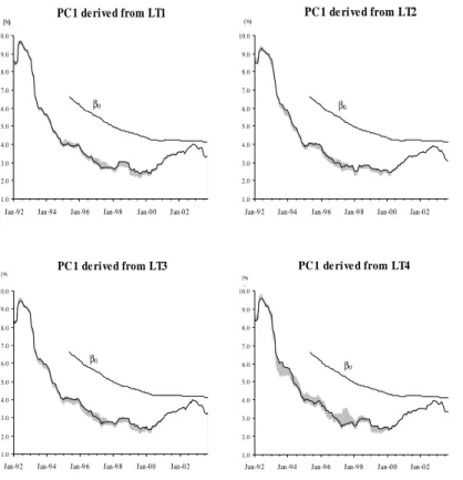
1.0 2.0 3.0 4.0 5.0 6.0 7.0 8.0 9.0 10.0

Jan-92 Jan-94 Jan-96 Jan-98 Jan-00 Jan-02 PC1 derived from LT1 (%) β0 1.0 2.0 3.0 4.0 5.0 6.0 7.0 8.0 9.0 10.0

Jan-92 Jan-94 Jan-96 Jan-98 Jan-00 Jan-02

(%) PC1 de rived from LT2 β0 1.0 2.0 3.0 4.0 5.0 6.0 7.0 8.0 9.0 10.0

Jan-92 Jan-94 Jan-96 Jan-98 Jan-00 Jan-02

(% ) PC 1 de rived from LT3 β0 1.0 2.0 3.0 4.0 5.0 6.0 7.0 8.0 9.0 10.0

Jan-92 Jan-94 Jan-96 Jan-98 Jan-00 Jan-02

(% )

PC1 de rive d from LT4

β0

Figure 2 - OLS results within the recursive procedure (I)

fundamentally unstable against the previous scaled result.

A second general approach was to evaluate if, along with another additional

observa-tion, the inner products under which the final OLS-scaled P C1 are being computed

incorporates some abnormal or unacceptable behaviour in time; for this purpose, the

partial derivatives of P C1 with respect to xi, i = 1,2, ...,90 were also disclosed and

analyzed.

Within the first general approach, the maximum and minimum values recorded in each month were firstly retrieved and plotted in figure (2). This was done for all transformations. For each month, the maximum and minimum values define the upper and lower limit of the grey region. The differential between those limits acts

as an indication of how much the _core inflation level has changed (for each month)

within the 91 sets of final OLS-scaledP C1. The core inflation indicator, using the full

sample period, and the evolution in time of β0 of equation (3), during the recursive

computation, were also depicted.

maximum (Max) and the sum (Sum) of the differential between the upper and lower

core inflation levels of each month (in basis points). As it can be seen, the

differ-ences cannot be considered very substantial and once again cannot be used to clearly distinguish between the transformations. The exception is perhaps LT4. Using the

full set of recursive estimates, the reported statistics have higher levels _vis-`a-vis the

other transformations.

Av Stdev Max Sum Av Stdev Max Sum

LT1 21 12 47 2928 LT3 22 13 53 3149

LT2 21 13 47 2979 LT4 34 25 104 4801

It should be clear that one of the reasons behind such close results derives from the

fact that all _core inflation indicators have the same mean. If the overall mean is

non-stationary and changes from CP I(T) to CP I(T+1), it will always be CP I(T+1)

that will be the relevant mean underlying the systematic use of equation (3), and not

CP I(T)

, implying that the mean of the _core inflation indicator will not diverge, by

construction, and over any sample period, from the mean of the observed inflation

rate. Given that β0 is added in the end of the process, as additional observations

are being disclosed, the use of (3) simply adapts the fact that in the Portuguese

case the mean of the inflation rate has decreased over time (as registered by β0 in

the graph). With no differences in the mean, the only possible way to differentiate between the linear transformations has to be based on the inner products under which

the OLS-scaled P C1 are being derived. The inner products depend upon three types

of scalars: (i) the scaling constant β1, (ii) the scalars defining the first eigenvector

and (iii) the scalars defining the transformation of the original variables. With one

additional observation, any one of these scalars may change. Let [P C1]_xi be the

partial derivative of the P C1 with respect to the original variable xi. From (2) and

(3),

[P C1]_xi =β1 ai1 hii−1, i= 1,2, ..., N. (4)

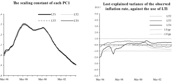
The scaling constants β1 of LT1, LT2, LT3 and LT4 were also computed and plotted

in the left panel of figure (3). For comparison purposes, the eigenvectors were scaled

to the inverse of their roots. As it can be seen, β1 has not remained unchanged over

1,8 1,9 2,0 2,1 2,2 2,3 2,4

Mar-96 Mar-98 Mar-00 Mar-02 LT1 LT2

LT3 LT4

The scaling constant of e ach PC 1

-5.0 -4.0 -3.0 -2.0 -1.0 0.0 1.0 2.0 3.0 4.0 5.0

Mar-96 Mar-98 Mar-00 Mar-02 LT2 LT3 LT4 1.0 pp -1.0 pp

Lost e xplaine d variance of the obse rve d inflation rate , against the use of LT1

(p.p.)

Figure 3 - OLS results within the recursive procedure (II)

again virtually the same in practice. In all cases, β1 follows an initial upward trend,

reaching a maximum in the first half of 1998 and then follows in general a downward

trend until the end of the sample period. The lost variance of the CP I for having

chosen LT1 and not LT2, LT3 or LT4 was also computed and plotted in the right panel of figure (3). Within each sample period, this lost variance is being defined as (β2

1 −βLT i2 )/σ_{CP I}2 , where β12 is being derived from LT1, βLT i2 is being derived from

LT2, LT3 or LT4 (a negative sign indicates a loss against the use of LT1) andσ2

CP I is

the variance of the inflation rate. In general, the percentage variance of the overall

inflation rate that is being captured by the first P C, derived from LT1, is most of

the times less than 1 percentage points away from the other possibilities.

The inner products of [P C1]_xi were further investigated and the following course of

action was implemented. In a first step, the results obtained during the computation

of the ninety one sets of core inflation indicators were separated into (i) N scalars

defining the first eigenvector (the a_i1) and (ii) N multiplying scalars of the original

variables associated to each transformation (the h−_ii1). In a second step, for

com-parison purposes, the a1 and the h−_ii1 obtained in (i) and (ii) were scaled under the

restriction that their sum would equal one, respectively, i.e. ΣN

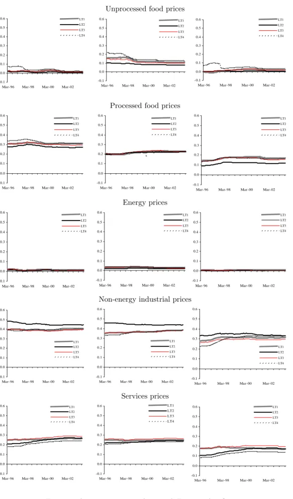
i=1ai1 = ΣNi=1h−_ii1 = 1. As a third step, the disaggregated results obtained in the second step were aggre-gated (added) according to the Eurostat classification of unprocessed food, processed food, energy, non-energy industrial goods and services prices. Without any scaling,

results are just equal to the sum of each β1 ai1 hii−1 belonging to the same Eurostat aggregate).

The behaviour over time of the Eurostat aggregates steming from LT1, LT2, LT3 and LT4 were plotted in the next 5 rows of figure (4). In each figure, the graphs on the left

correspond to the results for the first eigenvector (the scaled a_i1); the graphs on the

center correspond to the results for the scalars with an effect on the importance of the

original variables (the scaled h−1

ii ); the graphs on the right correspond to the results

for the final partial derivatives affecting the original variables (the β1 ai1 hii−1).

Several conclusions may be drawn from those figures. First, energy prices are treated in a rather indistinguishable way in all cases. Second, all transformations share the common internal features, in the end of the process, of (i) attaching a lower im-portance to those original variables belonging to the same aggregates (Energy and Unprocessed Food), and (ii) favour those of non-energy industrial goods. Third, LT4 does effectively seem to incorporate a higher variability then the remain

transforma-tions, but specially when the P C1 is derived with fewer observations. In the case of

LT2, it should be mentioned that the partial derivatives associated with processed food prices sum up to a lower level, as compared to the remaining transformations; and services items have received a growing importance over time. Using the full sample period, the differences against LT1 are almost non-existent in the case of unprocessed food, energy and services prices. Finally, the non-stationarity feature of the original data is not having any noticeable undesirable and distinctive effect

on the final partial derivatives of any of the transformations (including under LT18_).

Nor can it be used to clearly distinguish the overall results.

The empirical evidence therefore suggests that, under all the transformations consid-ered, the importance of each original variable is being relatively changed in such a way that the final results do empirically emerge as similar and hard to distinguish (which is particularly striking, given that no justification was given to implement LT3 or LT4). Although each transformation may qualitatively change the eigenvalues/eigenvectors solution of the original maximization problem, the use of structurally different linear transformations do not produce, clearly, dissimilar final results. In the case of LT1,

8_{It may also be the case that the non-stationarity of the original data is basically creating a correlation matrix}

with a large number of positive elements, as the variables are somehow moving in the same directions, and to some extent the evolution of the first eigenvector over the different sample periods may only be reflecting what is usually referred to as a “size effect”. See Chatfield and Collins (1996) and Jollife (2002). During the different sample periods, the number of positive elements of the second moment matrix stood always between 75 and 80 per cent.

Unprocessed food prices -0.1 0.0 0.1 0.2 0.3 0.4 0.5 0.6

Mar-96 Mar-98 Mar-00 Mar-02

LT1 LT2 LT3 LT4 -0.1 0.0 0.1 0.2 0.3 0.4 0.5 0.6

Mar-96 Mar-98 Mar-00 Mar-02

LT1 LT2 LT3 LT4 -0.1 0.0 0.1 0.2 0.3 0.4 0.5 0.6

Mar-96 Mar-98 Mar-00 Mar-02

LT1 LT2 LT3 LT4

Processed food prices

-0.1 0.0 0.1 0.2 0.3 0.4 0.5 0.6

Mar-96 Mar-98 Mar-00 Mar-02

LT1 LT2 LT3 LT4 -0.1 0.0 0.1 0.2 0.3 0.4 0.5 0.6

Mar-96 Mar-98 Mar-00 Mar-02

LT1 LT2 LT3 LT4 b -0.1 0.0 0.1 0.2 0.3 0.4 0.5 0.6

Mar-96 Mar-98 Mar-00 Mar-02

LT1 LT2 LT3 LT4 Energy prices -0.1 0.0 0.1 0.2 0.3 0.4 0.5 0.6

Mar-96 Mar-98 Mar-00 Mar-02

LT1 LT2 LT3 LT4 -0.1 0.0 0.1 0.2 0.3 0.4 0.5 0.6

Mar-96 Mar-98 Mar-00 Mar-02

LT1 LT2 LT3 LT4 -0.1 0.0 0.1 0.2 0.3 0.4 0.5 0.6

Mar-96 Mar-98 Mar-00 Mar-02

LT1 LT2 LT3 LT4

Non-energy industrial prices

-0.1 0.0 0.1 0.2 0.3 0.4 0.5 0.6

Mar-96 Mar-98 Mar-00 Mar-02

LT1 LT2 LT3 LT4 -0.1 0.0 0.1 0.2 0.3 0.4 0.5 0.6

Mar-96 Mar-98 Mar-00 Mar-02

LT1 LT2 LT3 LT4 -0.1 0.0 0.1 0.2 0.3 0.4 0.5 0.6

Mar-96 Mar-98 Mar-00 Mar-02

LT1 LT2 LT3 LT4 Services prices -0.1 0.0 0.1 0.2 0.3 0.4 0.5 0.6

Mar-96 Mar-98 Mar-00 Mar-02

LT1 LT2 LT3 LT4 -0.1 0.0 0.1 0.2 0.3 0.4 0.5 0.6

Mar-96 Mar-98 Mar-00 Mar-02 LT1 LT2 LT3 LT4 -0.1 0.0 0.1 0.2 0.3 0.4 0.5 0.6

Mar-96 Mar-98 Mar-00 Mar-02

LT1 LT2 LT3 LT4

the sum of the partial derivatives belonging to the each aggregate has remained

rela-tively stable in time and no obvious gain is apparently achieved by changing the _core

inflation indicator, as proposed in Coimbra and Neves (1997), for any other of the remaining possibilities. On the contrary, under LT2, LT3 or LT4, the quantity under maximization ceases to be a standard and well perceived statistic, i.e, without a clear advantage, the input variables cease to be treated as “equally important” variables, as in the case of LT1. It may be argued that standardization has only an immediate

statistical interpretation when the input variables are stationary.9 However, all four

transformations herein applied do not change the non-stationarity feature of the orig-inal database. It is only a matter of different scaling of the origorig-inal variables and of different second moment matrices. Whereas under LT2, LT3 or LT4, these matrices are somehow more difficult to interpret, under LT1 the second moment matrix is the rather straightforward correlation matrix. By conveying a well known information, the overall process becomes apparently more easily perceptible and intuitive.

3

On the use of non-contemporaneous variables

The common factors can be derived not only from contemporaneous but also from

non-contemporaneous values of X. So far, the P C_i has only been derived from

contemporaneous data and therefore a possible improvement of this _core measure

could be to allow for some dynamics, along the lines suggested for instance by Stock and Watson (1998), or Stock and Watson (2002).

Following the same recursive procedure introduced in the previous section, the _core

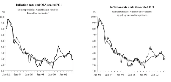
inflation indicator can now be derived from equation (3), but after having stacked non-contemporaneous figures to the original database. Figure (5) reports the results

for all OLS-scaled P C1, conditional on LT1, where the grey region is limited, as in

the previous section, by the maximum and minimum values obtained for each month. The left panel of figure (5) considers contemporaneous variables and variables lagged

by one period, the right panel also considers variables lagged by two periods.10

As before, these results do not seem highly different from the ones obtained by only using contemporaneous variables in the database, except that the inflation indicator

9_{Alexander (2001) goes even further and declares that the data input of Principal Component Analysis “must be}

stationary” (p. 145). On this issue, see also Machado et al. (2001).

10_{With contemporaneous variables and variables lagged by one and two periods, the number of input data is now}

1,0 2,0 3,0 4,0 5,0 6,0 7,0 8,0 9,0 10,0

Jan-92 Jan-94 Jan-96 Jan-98 Jan-00 Jan-02

Inf lation rate and OLS-scaled PC1

(contemporaneous variables and variables lagged by one period) (%) 1,0 2,0 3,0 4,0 5,0 6,0 7,0 8,0 9,0 10,0

Jan-92 Jan-94 Jan-96 Jan-98 Jan-00 Jan-02

(%)

Inf lation rate and OLS-scaled PC1

(contemporaneous variables and variables lagged by one and two periods)

Figure 5 - OLS results within the recursive procedure (III)

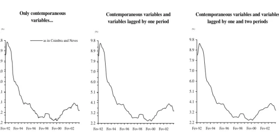
is now smoother (see figure (6)). The standard deviation of the first difference of the

OLS-scaledP C1, using the full sample period, falls from 0.17 in the contemporaneous

case, to 0.14 with one lag and to 0.13 with two lags.11 _{The following table contains}

the average, the standard deviation, the maximum and the sum of the differentials, as in the previous section. In all cases, the sum of the differentials obtained for each month is also lower than in the contemporaneous case.

Av Stdev Max Sum

Contemporaneous and lag1 21 11 43 2881

Contemp., lag1 and lag2 21 11 40 2863

Contemp., lag1, lag2 and lag3 21 11 41 2863

Nevertheless, unless a smoother core inflation indicator is being envisaged on_{a priori}

grounds, no obvious gain seems to be achieved by changing the currently used pro-cedure at the Banco de Portugal (as in the previous section), specially if the shocks that hit the economy are themselves not smooth or if the transmission of the effects

of these shocks onto prices is changing.12 Furthermore, this possible strategy requires

that some type of non-contemporaneous dynamic structure as to be superimposed on the original data. In the above examples, one, two or three lags were just arbitrarily considered and analyzed. On the other hand, if leads are also to be considered as

11_{Although the empirical results reported in this section are all conditional on LT1, it should be mentioned that}

the differences between LT1 and the transformations anayzed in the previous section are again very small. In the case of LT2, LT3 and LT4, the results were 0.135, 0.159 and 0.168, respectively. Using h_ii=σ_∆2_xi, whereσ_∆2_xi

represents the standard deviation of the second difference ofx_i, the result would have been 0.138.

12_{See Mankikar and Paisley (2002). On the desirable properties of a measure of “core” inflation, see, for instance,}

2.2 3.2 4.1 5.1 6.0 7.0 7.9 8.9 9.8

Fev-92 Fev-94 Fev-96 Fev-98 Fev-00 Fev-02 as in Coimbra and Neves

Only contemporaneous variables... (%) 2.2 3.2 4.1 5.1 6.0 7.0 7.9 8.9 9.8

Fev-92 Fev-94 Fev-96 Fev-98 Fev-00 Fev-02

Contemporaneous variables and variables lagged by one period

(%) 2.2 3.2 4.1 5.1 6.0 7.0 7.9 8.9 9.8

Fev-92 Fev-94 Fev-96 Fev-98 Fev-00 Fev-02

(%)

Contemporaneous variables and variables lagged by one and two periods

Figure 6 - OLS results within the recursive procedure (IV)

input variables and unless some projections can be used, it is clear that the _core

inflation indicator ceases to be a real time index (not computable until t=T).

4

On the use of more than one principal component

Within the principal components methodology, i.e., behindP C = (X−X)H−1_{A, the}

objective is to find “clean”, orthogonal (uncorrelated) variables, which are extracted from noisy and possibly highly correlated original variables. It may be the case that a large percentage of the total variance present in the system might be retained by

a few P C_i and, in this sense, the effective dimensionality of the original information

set may be substantially reduced. Within factor analysis, the objective may be seen as having the inverse direction. It may be the case that the main internal features of a given set of variables may be captured by a small number of unobservable variables - the common factors. It is therefore crucial to the correct specification of the factor model the use of an adequate number of factors. Several proposals may be found in

the literature to properly determine, from the observed data, the number of factors.13

A classical way to determine the number of principal components that should be

retain as factors simply relies on the contribution of each P C_i to the total variation

present in the system. If the eigenvalues and eigenvectors (scaled to unity) are

ex-tracted from the correlation matrix ρ_X, the appealing feature of ΣN

i=1V ar[P Ci] =

ΣN

i=1λi =tr(Λ) =tr(ρ) =N is valid, where a descending order of the eigenvalues has

0,5 0,6 0,7 0,8 0,9 1,0

Mar-96 Mar-98 Mar-00 Mar-02 PC1 PC2 PC3 PC4 PC5 PC6 Pe rce ntage of total variance accounte d

for by 6 PC i 49.9% 58.6% 64.9% 69.6% 74.1% 77.5% 0% 20% 40% 60% 80% 100% l1 l2 l3 l4 l5 l6 Cumulated M arginal

Pe rce ntage of total variance accounte d for by 6 PC

Figure 7 - On the use of more then one principal component (I)

a direct link with a descending order of variance accounted for by their respective

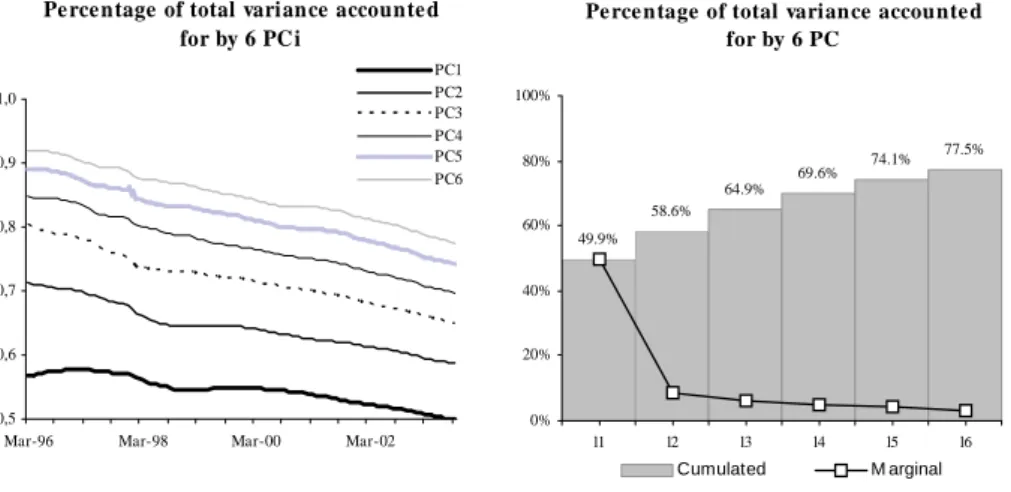
P Ci. The results of up to 6 P C were gathered and plotted in figure (7). From the

graph on the left, the percentage variance accounted for by theP C1has never reached

60%, during the computation of the 91 _core inflation indicators (already introduced

in the previous sections), and has somehow evolved along a downward trend.14 In the

end of the sample period (see graph on the right), with T = 141, it stood at 49.9%.

As expected, the inclusion of more P C_i increases this percentage, with marginally

decreasing contributions (for instance, using all observations, P C2 accounts for 8.7%

of the total variance present in the system; P C3 accounts for 6.3%; P C4 for 4.7%).

With the aim of capturing more variance of the observed inflation rate, it might

therefore be suggested that the _core inflation indicator should be derived not only

from the first, but probably from two or more P C_i. Coimbra and Neves (1997) or

Machado et al. (2001) simply seem to assume the need for one factor and, in fact, there are several reasons to maintain this option. A first reason is based on the relevant

information criteria under which the number of retained P C_i is determined. In fact,

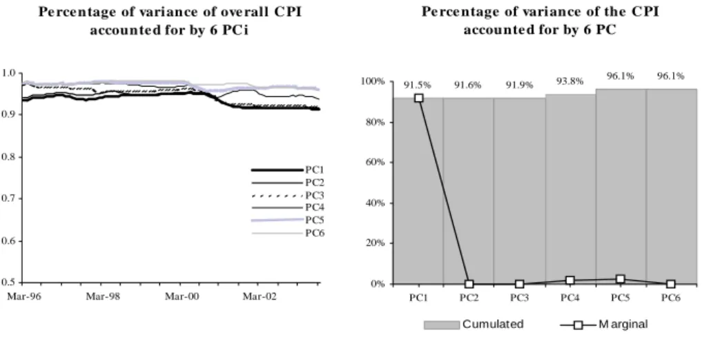
although a slight downward trend was also detected, the OLS-scaled P C1 has always

captured a high percentage of the variance of the overall inflation rate, as illustrated in the left panel of figure (8). In the end of the sample period (see right panel), it stood

at 91.5%. Therefore, the general driving behaviour of the CP I is being captured,

to a large extent, by one single P C, and the contribution of the remaining ones is

negligible. Moreover, a descending order of λ_i has no direct link with a descending

14_{The percentage of total variance accounted for by theithP Ccan be sought as} λi tr(Λ) =

λi

N, which evolves in time

0.5 0.6 0.7 0.8 0.9 1.0

Mar-96 Mar-98 Mar-00 Mar-02 PC1 PC2 PC3 PC4 PC5 PC6

Pe rce ntage of vari ance of ove rall C PI accounte d for by 6 PC i 91.5% 91.6% 91.9% 93.8% 96.1% 96.1% 0% 20% 40% 60% 80% 100% PC1 PC2 PC3 PC4 PC5 PC6 Cumulated M arginal

Pe rce ntage of vari ance of the C PI accounte d for by 6 PC

Figure 8 - On the use of more then one principal component (II)

order of the variance accounted for by the respective OLS-scaledP C_i.15 _{For instance,}

the variance of the OLS-scaledP C4 is higher than the variance of the OLS-scaledP C2

or P C3. Therefore, marginal gains would be obtained from including, successively,

the P C_i with i = 1,2 and 3, and a sudden larger gain is obtained when the

OLS-scaled P C4 is also included. This result, which simply implies a clear approximation

of the “core” inflation to the observed inflation, is basically explained by the fact that

a higher variance accounted for by a specific P C_i (obtained from eigenvectors scaled

to unity) may be abruptly reduced or increased by its respective OLS-scaling.

Another related reason to reject the possibility of including more than theP C1 in the

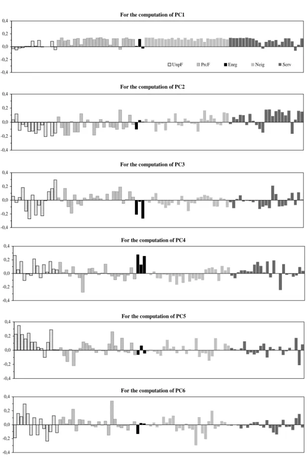
computation of the_coreinflation indicator is based on the analysis of the eigenvectors.

Using the full sample period, the scalars defining the first six eigenvectors (scaled to unity) were plotted in figure (9). With few exceptions, the scalars associated to the first eigenvector have all basically the same sign (non-negative), whereas the scalars associated to the remaining eigenvectors oscillate quite substantially between

positive and negative signs.16 _{This implies that the different P C}

i may be capturing

different phenomena and therefore some additional explanation will have to be put

forward so as to include more the first principal component.17 _{By taking advantage}

of the positive correlations found in the database, positive a_i1hii−1 simply implies

that higher year-on-year rates of change of specific items of the CPI are associated

15_{This is not surprising given that the variance of theP Ciis dependent upon the scaling of the eigenvectors. For}

instance, under eigenvectors scaled to the inverse of their roots, the link with the descending order of the (respective) λidoes not exists, since the variances of eachP C_iare always equal to one.

16_{The negative signs in the case ofP C1were already mentioned in Machado et al. (2001).}

17_{An example where theP C1, theP C2 and theP C3 are used to capture three different effects may be seen in}

Eigenvectors scaled to unity -0,4 -0,2 0,0 0,2 0,4

UnpF PrcF Enrg Neig Serv

For the computation of PC1

-0,4 -0,2 0,0 0,2 0,4

For the computation of PC2

-0,4 -0,2 0,0 0,2 0,4

For the computation of PC3

-0,4 -0,2 0,0 0,2 0,4

For the computation of PC4

-0,4 -0,2 0,0 0,2 0,4

For the computation of PC5

-0,4 -0,2 0,0 0,2 0,4

For the computation of PC6

with higher scores of the principal component. Moreover, it will be seen in the next

section that the small number of negative signs in the case of the P C1 can also assure

that β1 of (3) will most probably be positive, whereas the sign and the magnitude in

the remaining cases is largely unknown.

5

The OLS scaling of the principal components solution

The estimation of factor scores, common to all variables present in the system, using

unweighted ordinary least has been a customary procedure18_{and the previous section}

has in fact computed the OLS fitted values of (3) in order to have a core inflation

indicator with comparable scores to those of the CP I. Along with other properties,

this so called _“ad-hoc” procedure19 can now have a well defined interpretation if the

system of equations (1) also incorporates the fact that the CP I is also a [T ×1]

vector where CP I = ΣN_i=1α_ix_i = Xα. Derived from some household budget survey,

αi are the consumption basket weights of each item and ΣNi=1αi = 1. In this case,

note that x_i is a price index and not a price change. If thex_i are previously centered:

(CP I −ΣN_i=1α_ix_i) = (CP I −CP I) = (X−X)α. Let CP I represent the average of

the CP I index.

For simplicity reasons, assume that (2) was written down with price indices and that

H is equal to the identity matrix, i.e. the principal components were derived from

Σ_X. It is well known that from P C = (X−X)A, the full [T ×N] matrix X can be

reproduced without error through a principal components representation

X =X+P CA−1 (5)

If the eigenvectors a_i included inA were scaled to unity, the variance of their

respec-tive P C_i will be given by λ_i and A−1 _{of (5) is equal to A. However, the variance}

of each P C_iis fundamentally undetermined as each a_i may be scaled to any

con-stant c_i, i.e., to a_ia_i = c_i, which implies that V ar(P C_i) = a

iΣXai = ciλi. Unless

other considerations are brought into the computational process, choosing a_ia_i = 1

and V ar(P C_i) = λ_i is just one of the possible options. Let P C_iU represent the ith

principal component obtained from unit length eigenvectors.

After having unfolded the matrix A and using, for simplicity reasons, unit length

18_{See, for instance, Johnson and Wichern (2002).} 19_{See Coimbra and Neves (1997,p.31).}

eigenvectors, it can now be showed that both the CP I, and its overall variance (σ2

CP I) can also be reproduced without error through a principal components

struc-ture. Algebraically, the initial linear combination of the original variables, i.e., the

overall CP I, is just going to be expressed as a linear combination of another set of

vectors. From (5), the entire [T ×N] matrix X collapses to a single equation for

the CP I and, with a principal component solution, the following orthogonal factor

model emerges CP I =Xα= (X+P CUA)α= CP I+ ΣN i=1P CiUaiα (6) and, as expected, V ar[CP I] ≡σ2 CP I =V ar[P CUAα] = [αA P CU][P CU Aα] = [αAΛAα] =αΣXα

In short, the overall CP I index and its variance can be exactly reproduced within an

orthogonal factor model framework with as many common factors (principal compo-nents) as variables. Thus, without any assumption on the data generation process of

each variable, theCP I is not only a product of the aggregation of all its basic items;

it is also a product the all its scaled principal components. Moreover, if only p < N

principal components are retained within this framework, this will produce an index

(by construction) with comparable scores as those of the observed overall CP I (it

will have, namely, the same average), but with a smaller variance. Those retained

P C will now account for a certain percentage of the overall variance of the CP I,

which is a different quantity against the accounted percentage of the total variance present in the system.

It turns out that equation (6) not only represents a solution for the fundamental eigenvectors length indeterminacy, but also uniquely determines the variance of the

CPI accounted for by each P C_i.20 _{Model (6) surpasses the problem of having to}

choose a particular eigenvector length to solve the initial problem Σ_Xa = λa, given

that all possible choices can be proved to collapse to (6). Changing the length of an

eigenvector will change the variance of the P C_i but this will also functionally change

the scaling constant and the inner product of both will, most conveniently, remain

unchanged. Under this result, the percentage variance of the CP I accounted for

by these products is not conditional on the eigenvectors length.21 Using unit length

20_{The proofs are included in Annex 2.} 21_{Each productP C}U

i aiαis therefore independent of the eigenvector’s length (aiαis the result of an inner product

eigenvectors, V ar[CP I] can be further subjected to the following breakdown.

V ar[CP I]≡σ2

CP I = ΣNi=1V ar[P CiU](αaiaiα) = ΣNi=1λi(αaiaiα)

Within this framework, the use of one or several P C_iU can be easily scrutinized and

naturally allows to classify any _core inflation indicator steaming from this

specifica-tion to be, by construcspecifica-tion, a “trimmed variance” index (to use an expression from the trimmed mean literature). Finally, it is relevant to point out that equation (6) is

fully equivalent to an OLS scaling. A regression between theCP I and theP C_i

struc-ture, i.e. CP I =β0+β1P C1U+...+βNP C_NU+ε will pre-determine thatβ0, β1, ..., βN

will be equal to the above results CP I, a₁α, ..., a_Nα, respectively, and, in this case,

ε= 0.22 _{By construction,}

(P CUP CU)−1P CUCP I = (P CUP CU)−1P CU(P CUA)α = a₁α a₂α ... a_Nα

Assume for now that the_core indicator (CP IT) was defined as the OLS fitted values

of CP I = β0 +β1P C1U +ε (i.e. it only uses the first P C). It is now clear that

this specification is not _{ad hoc} and, instead, has the following consequences: (i) the

CP IT _{is pre-determined and is equal to CP I +a}

1αP C1, as the PC are orthogonal;

(ii) V ar[CP IT] is pre-determined and is equal to λ1(αa1a1α), where V ar[CP IT]

represents part of the variance of the overall CP I that is being captured;23 (iii)

ε = ΣN

i=2aiαP Ci is ignored; and, as a consequence, (iv) V ar[ε] = ΣNi=2V ar[P Ci]

(αa_ia_iα) is also ignored. The CP IT will be, by construction, smoother than the

CP I by an amount given by V ar[ε] as the CP IT is “trimming” the variance of the

CP I by a percentage given by ΣN

i=2λi(αaiaiα)/(σ_{CP I}2 ). V ar[ε] can be seen as the

ignored variability of the overall CP I against the variability of the CP IT.

After having established in the previous section that the _core inflation indicator

derived from the correlation matrix does emerge as a reasonable option, namely under non-stationary input variables, the OLS scaling can now be simply interpreted

as the appropriate linear combination of P C_i that replicates the observed inflation

rate. Given that the database that has been used so far is not made of indices but ones introduced in the first section, equation (6) would have to be modified. With unit length eigenvectors, P C= (X−X)H−1A⇔X =X+P CAH and thereforeCP I=CP I+P C1a1Hα+...+P CNaNHα. Nevertheless, the

properties that were mentioned in the main text remain in place.

22_{It is now clear that if the scalars of the eigenvector are all positive, thana}

1αwill also be a positive scalar. Note

also that if the scalars of the eigenvector are all negative,β_iwill also be negative and therefore the product of both will reverse to a positive scalar.

23_{Using eigenvectors scaled to the inverse of their roots, and not to unity, can now be seen as most useful and}

highly appealing. Not only the final OLS fitted values of the regression do not change, as V ar[CP IT] is now simply obtained by β₁2. In general, with the principal component associated with this scaling denoted as P C_iW, V ar[CP I] =V ar[β₀+β₁P C₁W+...+β_NP C_NW] =β2₁+β₂2+...+β2_N.

of N year-on-year rates of changes, the restriction for the overall CP I index has to

be adapted for the rate of change of the overall CP I index. With monthly data,

this can be implemented by changing the database from x_it ≡(I_it −I_it−12)/I_it−12, to

xit ≡i×(Iit−Iit−12)/Iit−12, i.e., to contributions for the year-on-year rate of change

to the CP I. I_i is a specific price index,i= 1...N and _i = (I_it−12/CP I_t−12)×αi. In

this case, an OLS regression such as CP I· =β0+β1P C1U would simply collapse to

·

CP IT _{=CP I + (Σ}N

i=1ai1σi)P C1U (7)

where the data has been standardized, a_i1 represents the first eigenvector scaled

to unity, σ_i is the standard deviations of the new x_it, P C₁U is the first principal

component obtained from the first eigenvector scaled to unity, andCP I is the average

inflation rate.24 _{To put it differently, no OLS regression would have to be implemented}

and no parameter has to be estimated as a final stage for the determination of the

core inflation indicator if the length of the_jth eigenvector is not scaled to unity, but

to (ΣN

i=1ai1σi)2. The percentage of the overall variance of the rate of change of the

CP I that is being captured is given by V ar[CP IT]/σ_{CP I}2 , where V ar[CP IT] = (β₁2

λ1) = (ΣN_i=1ai1σi)2λ1. Under LT1 and with unit length eigenvectors, model (7) can

easily be expanded to

CP I = ΣN

i=1xit =CP I + (ΣNi=1ai1σi)P C1U+...+ (ΣN_i=1aiNσi)P CNU.

Moreover, as already mentioned, if the a_i are extracted from the correlation matrix,

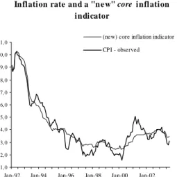
which is the case under LT1, this choice involves an arbitrary decision to make the variables “equally important”. The transformed variables will be indistinguishable from a “variance and location point of view”, as the diagonal elements of the cor-relation matrix are all unity. Using the new database, it also seems conceptually appealing to make the contributions and not the rates of change the “equally impor-tant variables”. An implementation of (7) may be found in figure (10).

The new database incorporates the weighting schemes associated to the House-hold Budget Surveys of 1989-90, 1994-95 and 2000, used for the calculation of the CPI(1991=100), CPI(1997=100) and the CPI (2002=100), respectively. As an im-provement against the previous core inflation indicators and with the objective of

widening the information contained in theP C1, the database was also expanded with

24_{If the P Ci are extracted from standardized data and the consumption basket weights remain unchanged over}

time, note also that the use of indices or weighted indices is a totally irrelevant issue, as it has no effect on the correlation matrix. Nevertheless, equation (6) can only be seen as an approximation for the specification in changes.

1,0 2,0 3,0 4,0 5,0 6,0 7,0 8,0 9,0 10,0 11,0

Jan-92 Jan-94 Jan-96 Jan-98 Jan-00 Jan-02 (new) core inflation indicator CPI - observed

Inflation rate and a "ne w" core inflation indicator

Figure 10 - Core inflation indicator derived from the contributions of CPI items

two additional variables related with housing expenditures (housing rents and prices

of maintenance and repair of the dwelling).25 As expected, the overall behaviour of

the observed inflation rate is once again being captured by this factor model.26

6

Conclusions

This paper has investigated if the (OLS-scaled) first principal component (P C1),

ex-tracted from standardized yearly rates of change of basic items of the CPI, represents

a reasonable option for a _core inflation indicator. Currently, the Banco de Portugal

uses this procedure to measure (and regularly publish) a _core inflation indicator for

the Portuguese case. A special focus was placed on the final stage of the process of

finding the _core indicator, in which theP C1 is subject to an OLS scaling, through a

regression of the CP I inflation rate on the CP1. The fitted values of this regression

- a so called _ad-hoc procedure - determines the _core inflation _level.

From the confrontation of structurally different linear transformations of the original data, including the one suggested by Machado et al. (2001), it was concluded that no obvious gain is clearly achieved by changing the standardization procedure for any other of the remaining possibilities. The overall final results of all transformations were not easily distinguishable, which may be seen as particularly striking given that two of those transformations were purely arbitrary and not motivated by any

25_{During the period 1992-1997, only annual observations are available. In line with the monthly behaviour that}

has been observed since 1997, it was therefore assumed that those annual figures were basically determined in the beginning of each year.

reason (except for comparison purposes). Even though most input variables are non-stationary, which was the main reason underlying the suggested transformation of Machado et al. (2001), the results were not find to be structurally dissimilar.

Secondly, if the objective is the find a smoother _core inflation indicator then the

one currently in use, then lagged variables can be stacked to the original database. However, it was also argued that unless other reasons are brought into the

deci-sion process, this increased smoothness does not seem to represent _{per se} a clear

superiority feature. Some type of non-contemporaneous dynamic structure as to be superimposed on the original data and if the shocks that hit the economy are not

smooth, why should the_core inflation indicator be smooth? In addition, the inclusion

of leads would prevent the indicator to be updated until the last period (abstracting from the possible use of some type of projections).

Finally, within a classical approach, the contents of the remaining principal compo-nents were also explored. Given that the main objective in the current analysis is to capture the general driving behaviour of the overall inflation rate, and not the total

variance present in the system, the conclusion was that a single component (theP C1)

seems sufficient. In the last 91 estimates, the OLS-scaled P C1 has always captured

more than 90% of the total variance of the CP I. Moreover, it was claimed that the

other eigenvectors may be capturing other effects rather than the “trend component”.

The sign and the magnitude of the OLS scaling of the remaining P C_i is also largely

unknown.

In general, the empirical evidence incorporated throughout this paper does suggest

that the OLS-scaled P C1, extracted from standardized yearly rates of change of basic

items of the CPI, does represent a reasonable option for a _core inflation indicator.

Moreover, it was showed that no OLS parameter has to be estimated as a final

stage of the process of finding the _core indicator. Instead of being seen as an

ad-hoc procedure, the OLS scaling can simply be interpreted as an appropriate linear

combination ofP C_i that replicates the observed inflation rate. To such purpose, this

paper introduced an orthogonal factor model that fully reproduces theCP I, in which

the following properties apply: (i) the results are not conditional on the eigenvectors

length; (ii) the variance of the CP I accounted for by each component is unique, and

as explanatory variables. The model was written down in price levels and in price changes (yearly rates) and this has given a clear interpretation to the OLS scaling.

To achieve these results, it is only necessary to respect the fact that the CP I can

be written down as a linear combination of the input data. In the latter case, under standardization, it would be the contributions and not the rates of change that could

be made “equally important variables” (which implies that the weights of the CP I

have to be fully taken into account for the determination of the CP1) and no OLS

regression has to be implemented (given that the final results are fully equivalent to a well defined scaling of the first eigenvector).

References

Afifi, A. A. (1984), _{Computer-Aided Multivariate Analysis}, Lifetime Learning.

Alexander, C. (2001), _{Market Models}, Wiley.

Angelini, E., Henry, J. and Mestre, R. (2001_a), Diffusion index-based inflation

fore-cast for the euro area, Working Paper 61, European Central Bank.

Angelini, E., Henry, J. and Mestre, R. (2001_b), A multi country trend indicator for

euro area inflation: Computation and properties, Working Paper 60, European Central Bank.

Bai, J. and Ng, S. (2002), ‘Determining the number of factors in approximate factor

models’, _Econometrica 70, 191–221.

Carroll, J. D. and Green, P. E. (1997), _{Mathematical Tools for Applied Multivariate}

Analysis, Academic Press.

Chatfield, C. and Collins, A. (1996),_{Introduction to Multivariate Analysis}, Chapman

and Hall.

Coimbra, C. and Neves, P. D. (1997), Indicadores de tendˆencia de infla¸c˜ao, Boletim

Econ´omico, Banco de Portugal. (March 1997).

Cristadoro, R., Forni, M., Reichlin, L. and Veronese, G. (2001), A core inflation index for the euro area, Temi di discussione 435, Banca D’Italia.

Jackson, J. E. (1991), _{A User’s Guide to Principal Components}, Wiley.

Johnson, R. A. and Wichern, D. W. (2002),_{Applied Multivariate Statistical Analysis},

Prentice Hall.

Jollife, I. (2002), _{Principal Component Analysis}, Springer.

Krzanowski, W. (1996), _{Principles of Multivariate Analysis - A User’s Perspective},

Oxford University Press.

Machado, J., Marques, C. R., Neves, P. N. and Silva, A. G. (2001), Using the first principal component as a core inflation indicator, Working Paper WP 9/01, Banco de Portugal.

Mankikar, A. and Paisley, J. (2002), What do measures of core inflation really tell us?, Quarterly bulletin, Bank of England.

Marques, C. R., Neves, P. D. and Sarmento, L. M. (2000), Evaluating core inflation indicators, Working Paper WP 3-00, Banco de Portugal.

Stock, J. H. and Watson, M. W. (1998), Diffusion indexes, Working Paper 6702, NBER.

Stock, J. H. and Watson, M. W. (2002), ‘Macroeconomic forecasting using diffusion

Annex 1

1 UnpF x1 Potatoes and other tubers 1 Neig x42 Garments (man)

2 x2 Beans and grains 2 x43 Garments (woman)

3 x3 Vegetables 3 x44 Clothes (babies)

4 x₄ Fruits 4 x₄₅ Clothing accessories

5 x₅ Mutton and others 5 x₄₆ Clothing materials

6 x6 Pork 6 x47 Footwear (man)

7 x7 Cow meat 7 x48 Footwear (woman)

8 x8 Small meat parts and related items 8 x49 Footwear (children)

9 x₉ Sausage 9 x₅₀ Repairs to footwear

10 x₁₀ Poultry 10 x₅₁ Water supply

11 _x11 Fresh and frozen fish 11 _x52 Electric household appliances

12 x12 Sea food 12 x53 Non-electric household appliances

13 x13 Canned fish 13 x54 Furniture

14 x₁₄ Smoked fish other related items 14 x₅₅ Household textiles

15 x₅₆ Glassware, tablewater, kitch. Items

16 _x57 Kitch. utensils and related items

1 PrcF x15 Cereals 17 x58 Products used currently

2 x16 Flours 18 x59 Medicines

3 x₁₇ Pasta products 19 x₆₀ Medical materials

4 x₁₈ Bread and bakery products 20 x₆₁ Therap. appliances and equipment

5 _x19 Eggs 21 _x62 Purchase of vehicles

6 x20 Milk 22 x63 Sound and pictures related equip.

7 x21 Milk derivatives 23 x64 Newspapers and books

8 x₂₂ Oils 24 x₆₅ Non durable household goods

9 x₂₃ Fats 25 x₆₆ Durable household goods

10 _x24 Sugar and honey 26 _x67 Other articles

11 x25 Jam

12 x26 Biscuits

13 x₂₇ Cakes and related items 1 Serv x₆₈ Restaurants, caf´es and canteens

14 x₂₈ Confectionary 2 x₆₉ Clothing services

15 x₂₉ Cocoa and related items 3 x₇₀ Maintenance and repair

16 x30 Coffee and related items 4 x71 Medical and paramedical services

17 x31 Tea 5 x72 Services of medical auxiliaries

18 x₃₂ Sauce, spices and foodstuff n.e.c. 6 x₇₃ Other maintenance expendit.

19 x₃₃ Food related items 7 x₇₄ Other expenditure

20 x₃₄ Wine 8 x₇₅ Urban collect. pass. transp.

21 x35 Other alcohol beverages 9 x76 Suburban collect. pass. transp.

22 x36 Water 10 x77 Long distance collect. pass. transp.

23 x₃₇ Juices 11 x₇₈ Other public transp.

24 x₃₈ Tobacco 12 x₇₉ Postal services and telegraph

13 x₈₀ Telephone

14 x81 Education

1 Enrg x39 Gas 15 x82 Repair services

2 x₄₀ Electricity 16 x₈₃ Culture

3 x₄₁ Fuels and lubrificants 17 x₈₄ Recreational services

18 x₈₅ Radio fees and other services

19 x86 Other services

20 x87 Hotels

21 x₈₈ Package holidays

22 x₈₉ Games of chance