Lightweight Java Profiling with Partial Safepoints and Incremental Stack Tracing

Lightweight Java Profiling with Partial Safepoints and

Incremental Stack Tracing

Peter Hofer

David Gnedt

[email protected] [email protected]

Johannes Kepler University Linz, Austria

Hanspeter Mössenböck

[email protected]

Institute for System Software Johannes Kepler University Linz, Austria

ABSTRACT

Sampling profilers are popular because of their low and ad-justable overhead and because they do not distort the profile by modifying the application code. A typical sampling pro-filer periodically suspends the application threads, walks their stacks, and merges the resulting stack traces into a calling context tree. Java virtual machines offer a convenient interface to accomplish this, but rely onsafepoints,a synchro-nization mechanism that requiresallthreads to park in a safe location. However, a profiler is primarily interested in the running threads, and waiting for all threads to reach a safe location significantly increases the overhead. In most cases, taking a complete stack trace is also unnecessary because many stack frames remain unchanged between samples.

We present three techniques that reduce the overhead of sampling Java applications.Partial safepointsrequire only a certain number of threads to enter a safepoint and can be used to sample only the running threads. Withself-sampling,we parallelize taking stack traces by having each thread take its own stack trace. Finally,incremental stack tracingconstructs stack traces lazily and examines each stack frame only once instead of walking the entire stack for each sample. Our techniques require no support from the operating system or hardware. With our implementation in the popular HotSpot virtual machine, we show that we can significantly reduce the overhead of sampling without affecting the accuracy of the profiles.

Categories and Subject Descriptors

C.4 [Performance of Systems]: Measurement Techniques

General Terms

Experimentation, Measurement, Performance

Keywords

Java, Profiling, Monitoring, Safepoints, Sampling, Stack Trace, Calling Context Tree

Permission to make digital or hard copies of all or part of this work for personal or classroom use is granted without fee provided that copies are not made or distributed for profit or commercial advantage and that copies bear this notice and the full cita-tion on the first page. Copyrights for components of this work owned by others than ACM must be honored. Abstracting with credit is permitted. To copy otherwise, or re-publish, to post on servers or to redistribute to lists, requires prior specific permission and/or a fee. Request permissions from [email protected].

ICPE’15,Jan. 31–Feb. 4, 2015, Austin, Texas, USA.

Copyrightc 2015 ACM 978-1-4503-3248-4/15/01 ...$15.00. http://dx.doi.org/10.1145/2668930.2688038.

1.

INTRODUCTION

Profilers are valuable analysis tools that help performance engineers to understand the behavior of applications and to assess the contribution of individual components to the overall execution time. A profiler observes the execution of an application and measures the run time and/or call frequency of methods to generate an execution profile which indicates those methods where the most time is spent or those that are called most frequently. An engineer can use this information to spot bottlenecks and to apply optimizations where they are most effective. Profiling is also useful to guide compiler optimizations, to determine test coverage, or to identify code that is never used.

In contrast to “flat” profiles that attribute measurements simply to methods, no matter from where they are called, prior research has demonstrated the importance of adding dynamiccalling contextinformation to profiles [2, 3, 24, 25]. The calling context is the call chain from the root method to the executing method; in other words, it is astack trace. Calling contexts can be merged into a calling context tree

(CCT, [2]), which differs from a call tree in that it merges identical children (callees) of a node.

In general, there are two approaches for collecting calling contexts. Instrumenting profilers insert code snippets in methods to record calls in the CCT. This approach yields an exhaustive CCT, but the instrumentation can introduce significant overhead and distorts the measured method execu-tion times. Sampling profilers,on the other hand, periodically interrupt the application to take stack traces and then merge them into the CCT. This approach requires no instrumen-tation and typically causes significantly less overhead, but it can miss method invocations between samples and there-fore results in an approximate CCT with only statistically significant information. Our research focuses on profiling techniques with minimal overhead that are suitable for mon-itoring production systems, which is why we concentrate on the sampling approach.

The Java Virtual Machine Tool Interface (JVMTI, [18]) offers functionality for sampling calling contexts of Java applications. It is supported by all common Java VM imple-mentations and is therefore used by many Java profiling tools. Implementations of JVMTI rely onsafepointsfor sampling, a mechanism that was originally devised for garbage collection: the Java VM inserts checks for a pending safepoint operation in the application code. When a profiler requests a sample, the VM signals such a pending safepoint operation and then waits for all application threads to reach a safepoint check and park. As soon as all application threads are parked in a

safe state, the stack traces can be taken. However, waiting for all threads to park causes significant delays. Parking all threads is often not even necessary because profilers are primarily interested in the threads that are currently running. Furthermore, the compiler can decide to eliminate safepoint checks for performance reasons, which further increases the time that it takes until all threads have parked.

In our previous research, we described a scheduling-aware sampling approach for Java VMs that uses a mechanism of the operating system to copy stack fragments of the running application threads into a buffer for asynchronous analy-sis [11, 12]. While this approach achieves very low overheads, it requires specific capabilities of the operating system. In this paper, we present an alternative set of techniques that also significantly reduce the overhead of sampling, but are independent of operating systems and hardware. We im-plemented these techniques in Oracle’s HotSpot VM [19], a popular high-performance Java VM.

The main contributions of this paper are:

1. Withpartial safepointsandself-sampling, we describe novel techniques that reduce the sampling pause times and that can be used to target those threads that are actually running.

2. We describe a new sampling technique called

incre-mental stack tracing. It constructs stack traces lazily

instead of walking the entire stack for each sample. In-cremental stack tracing examines each stack frame only once and shares the collected data between multiple stack traces.

3. We discuss aspects of our implementation in the HotSpot VM, such as changes to the VM’s safepoint mechanism and special cases which must be handled for incremen-tal stack tracing.

4. We provide an extensive evaluation of our techniques, comparing their overheads and their CCTs with those from conventional JVMTI sampling. For the evaluation, we use the DaCapo suite and the Scala Benchmarking Project. We show that our techniques are faster without affecting the accuracy of the CCTs.

The rest of this paper is organized as follows: Section 2 in-troduces calling context trees as well as profiling with JVMTI using safepoints. Sections 3, 4 and 5 describe our three tech-niques for reducing the sampling overhead and for targeting only the running threads. Section 6 describes aspects of our implementation. Section 7 evaluates the overheads and the accuracy of our techniques. Section 8 examines related work, and Section 9 concludes this paper.

2.

BACKGROUND

2.1

Calling Context Trees

A flat execution profile that only shows the observed meth-ods and their total execution times is of limited value. Often, a performance problem does not originate in the hot methods themselves, but rather in their callers. For example, when profiling shows that a program spends too much time in a sorting method, a developer could conclude that this method is inefficient. However, it could also be the case that the program would rather benefit from better data structures

a b c u v u 1 1 3 2 2

Call Tree Calling Context Tree a b c u b v u c c u

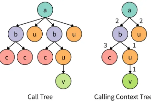
Figure 1: Call tree and calling context tree

that would reduce the necessary amount of sorting. The sorting method could be called from hundreds of locations in the program while the performance problem typically orig-inates in only a few call sites. To identify these call sites and to allow the developer to make changes where they have the most impact, profilers commonly sample entirecalling

contexts,which are stack traces from the executing method to

the root method (the entry point of the program or thread). Profilers typically represent all of the collected calling contexts in a tree structure, like a call tree. Figure 1 shows such a call tree, depicting, among others, multiple calls from

a to b, b to c, and a to u. The call tree represents each observed method invocation as a single node, with the caller as its parent. When the execution times of invocations are measured, they can be specified as edge weights. Call trees are an exhaustive representation of all calls of a program’s execution, but because each observed call introduces a new node, they quickly grow very large for most programs. Call trees are also less suitable for sampling profilers because these profilers typically cannot distinguish whether a stack frame seen in subsequent samples belongs to the same invocation or to different invocations of a method.

Calling context trees (CCT, [2]) are a more compact struc-ture than call trees. In contrast to call trees, CCTs merge identical children into a single node and thus store identical calling contexts only once. The edge weights specify the number of samples that were merged or the total execution times of all merged samples. A call tree can be converted to a CCT simply by recursively merging sibling nodes repre-senting calls to the same methods and adding up their edge weights. Figure 1 shows a call tree and its corresponding CCT. Since CCTs are more compact while still sufficiently expressive, CCTs are more common in practice.

2.2

Sampling with JVMTI and Safepoints

The Java Virtual Machine Tool Interface (JVMTI) is a native programming interface that allows debuggers, profil-ers, and similar tools to interact with the Java VM and the application running on top of it [18]. Clients of JVMTI are calledagentsand run in the same process as the Java VM. Agents can invoke JVMTI functions to control the behavior of the application and can register callbacks to receive no-tifications about application and VM events. For example, an instrumenting Java profiler would be implemented as an agent that subscribes to JVMTI’s class loading events and modifies the bytecode of classes when they are loaded.

Typical JVMTI sampling profilers start a separate agent thread that executes a sampling loop. In this loop, the pro-filer uses the JVMTI functionGetThreadListStackTraces

then processes these traces, for example by merging them into a CCT. It then goes to sleep for a certain time, referred to as the sampling interval, before repeating the process.

Because JVMTI offers ready-to-use functionality to ac-complish most of the sampling process (i.e., interrupting multiple threads, doing stack walks and decoding the stack frames to an array of method identifiers) sampling agents are straightforward to develop. However, the implementation of JVMTI in the HotSpot VM and in other VMs suffers from problems that affect the performance of sampling agents.

When an agent calls a JVMTI function for taking stack traces, the function does not start its work immediately, but rather enters a task into the work queue of the VM thread. The VM thread can be seen as the main thread of the virtual machine and is different from the application’s main thread. Only after higher-priority tasks in the queue have been completed, the VM begins taking stack traces.

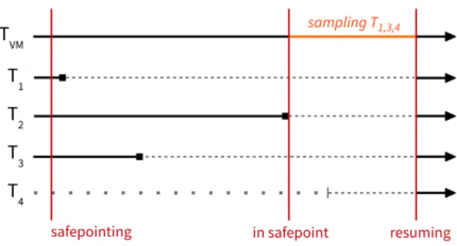
In order to safely walk the stacks of application threads, the VM relies on so-calledsafepoints.A safepoint is a state where all application threads are parked to allow safe execution of operations such as garbage collection, deoptimization, or stack walks. To accomplish this, the VM inserts checks for a pending safepoint operation at safe locations in the application code. When the VM thread signals a pending safepoint, each application thread enters a parking state after it runs to its next safepoint check. Threads that are already blocked, such as those that wait for an I/O operation, are always parked in a safe state and only need to enter a safepoint when they become unblocked while the safepoint is still in effect. Once all application threads are parked, the VM thread can safely take stack traces of threads. When the operation has finished, the VM leaves the safepoint, resumes all threads and passes the collected stack traces to the agent. Figure 2 shows an example of how JVMTI uses safepoints to sample application threads: ThreadTV Mis the VM thread, the threadsT1, T2 andT3 are runnable application threads,

and thread T4 is an application thread which is blocked

waiting to receive data via a socket. When the agent requests samples for the threadsT1,T3andT4, the VM thread begins

“safepointing”, i.e. it signals that a safepoint is pending. Soon after that, threadT1 reaches its next safepoint check and

enters a parking state (indicated by the square and the now dashed line), followed by thread T3. Thread T4 does not

have to enter a safepoint, since it is already blocked. At this point, threadT2 delays the process, although no sample

was requested for it, and threadsT1 andT3remain parked

and unproductive. When threadT3 finally parks and hence,

all threads have entered the safepoint,TV M can walk the stacks of the three threads requested by the agent. In the meantime, threadT4 becomes unblocked because its socket

has received data, but instead of resuming its execution, a safepoint check ensures that it also enters a parking state. After the VM thread has finished taking the stack traces, it ends the safepoint and resumes all application threads.

The main problem with using safepoints for sampling is that they affect all Java threads. Even the threads for which no stack trace was requested are required to run to their next safepoint and park until the stack traces have been collected. Hence, the entire application is paused even when only a single thread should be sampled.

Optimizations performed by the JIT compiler can further increase the performance impact of JVMTI sampling. By default, the compiler places safepoints at the exit points

safepointing in safepoint resuming

T₁ T₂ T₃ T₄ sampling T1,3,4 T_VM

Figure 2: Sampling threads in a safepoint

of methods and at the end of loop iterations. Although the overhead of safepoint checks is very low, it can become significant in hot loops. Safepoints also prevent certain kinds of optimizations because they enforce a particular order of instructions, similar to a memory barrier. Hence, the compiler can decide to move safepoints out of loops to increase performance and can even decide to eliminate safepoint checks in inlined code. With fewer safepoint checks, it can take longer until all threads are parked, and the sampling overhead increases. Eliminating safepoints also means that there are fewer locations where samples can be taken, which can distort the profile.

3.

PARTIAL SAFEPOINTS

Global “stop the world” safepoints are acceptable or even necessary for most purposes that they are used for, such as garbage collection and deoptimization. For a profiler, however, it is often sufficient to sample only a subset of the application’s threads. In fact, a profiler should focus particu-larly on the currently running threads because those are the ones that are actively consuming resources. Sampling these threads provides the most insight into where the program spends its time.

However, a sampling profiler that focuses only on running threads cannot be implemented with JVMTI and global safepoints. Although JVMTI supports restricting sampling to a set of threads, a sampling agent cannot determine a priori which threads will be running when the samples are taken. It is the operating system that schedules the threads, and common operating systems do not expose scheduling information to the VM or to an agent. The VM can only keep track of which threads arerunnable(i.e., ready to run). As an approximation, an agent could request samples for a selection of these threads. Still, this would not significantly decrease the sampling overhead because the safepoint would still affect all the other threads as well.

To target only running threads and to reduce the per-formance impact of sampling profilers, we implemented a variation of safepoints which we callpartial safepoints. Par-tial safepoints require only a certain number of application threads to enter a safepoint state. Samples are then only taken for these threads. We allow the agent to choose the number of threads to sample. By using the number of proces-sors in the system, sampling ideally affects only the running threads. With no scheduling data available, this is a best-effort approach. In practice, some of the system’s CPUs might be executing threads from other processes. Also, the operating system might interrupt a thread that was running when the sample was requested, and instead schedule another

thread which then enters the partial safepoint in its place. In the worst case, however, a sample is taken of a thread which was runnable, but not actually running, which we consider acceptable.

As soon as the intended number of threads has entered the partial safepoint, the VM can walk their stacks. Because some threads can enter a waiting state and block before reaching a safepoint check, we observe such thread state transitions to avoid a deadlock caused by waiting for more threads than can possibly enter the safepoint. While the stacks are walked, the safepoint must remain in effect. During that time, more threads than anticipated can enter the partial safepoint. Our implementation must consider which threads have entered the safepoint late and must finally resume all of them.

3.1

Waiting Threads

Samples of waiting threads can be useful to locate bottle-necks in locking or to detect inefficient I/O behavior. Threads blocked in a waiting state do not enter a safepoint unless they become unblocked while the safepoint is still in effect. This also applies to Java threads executing native code, where the VM ensures that a thread returning from native code enters a safepoint when one is in effect. Such native calls occur frequently because the Java class library implements I/O operations using native code, and these operations can also block.

We extended our partial safepoints mechanism with an option to take samples also of waiting threads and of threads that are in native code. If this option is active, we determine the number of runnable application threads and the number of threads that are waiting or executing native code, and accordingly divide the number of requested samples between runnable and waiting threads. For example, if a sampling agent requests four samples for an application that has 21 threads, out of which 15 threads are runnable and six threads are waiting or executing native code, our approach will return samples for the first three threads that enter the safepoint, and one sample for another, randomly selected thread.

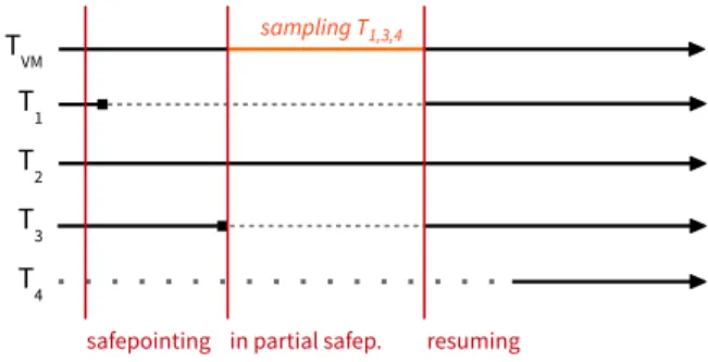
Figure 3 shows an example of how runnable and waiting threads are sampled with partial safepoints, using a similar scenario as the one shown in Figure 2. In this example, a sampling agent has requested three samples. The VM thread

TV M determines that there are three runnable threads and one waiting thread, and hence decides to sample two runnable threads and the waiting thread T4. TV M then signals a pending safepoint. As soon as two threads,T1 andT3, have

parked, it takes samples of their stacks and then immediately resumesT1 andT3. By the time when threadT2 reaches its

next safepoint check and whenT4 becomes unblocked, the

safepoint is no longer in effect, and their execution remains entirely unaffected by sampling.

4.

SELF-SAMPLING

With a straightforward implementation of partial safe-points, the safepoint remains in effect while the VM thread walks the stack of each thread to ensure that the stack walks can be done safely. During that time, further threads can enter the partial safepoint. Although these threads will not be sampled, they pause executing code, and the VM must also keep track of them in order to resume them later, all of which causes unnecessary overhead.

safepointing in partial safep. resuming

T₁ T₂ T₃ T₄

T_VM sampling T1,3,4

Figure 3: Sampling threads with a partial safepoint

sampling sampling safepointing in partial safepoint T₁ T₂ T₃ T₄ T_VM sampling T4 resuming

Figure 4: Self-sampling threads in a partial safepoint

To minimize the time the partial safepoint must remain in effect, we combined partial safepoints with a technique that we callself-sampling. When a thread enters a partial safepoint, it takes a ticket which tells it whether it is among the threads which should be sampled. If it is, the thread immediately walks its own stack. When the last thread that should be sampled enters the partial safepoint, it notifies the VM thread, which then signals the end of the safepoint so no further threads (which would not be sampled) can enter it. When a thread has completed sampling itself, it places the stack trace in a designated buffer and notifies the VM thread. The VM thread waits until all threads have provided their samples, and then resumes all sampled threads and returns the samples to the agent.

Because blocked threads do not enter a safepoint, they cannot sample themselves. Instead, the VM thread takes their samples, which increases the time the safepoint must remain in effect. However, the VM thread can take the samples while other threads are still running to their next safepoint check.

Figure 4 shows an example of a partial safepoint with self-sampling threads. As in Figure 3, the VM threadTV M inspects the states of the application threads, decides to sample two running threads and the waiting threadT4, and

then signals a pending safepoint. It then immediately begins to take a sample of the waiting threadT4. Meanwhile, the

threadT1enters the partial safepoint and examines its ticket.

Because it is the first of the two runnable threads that to be sampled, it walks its own stack, places the stack trace in the designated buffer and notifiesTV M. WhenT3 enters

the safepoint, it also examines its ticket and recognizes that it is the second and last of the two runnable threads to be sampled, so it notifies TV M, which signals the end of the safepoint. AfterT3 has sampled itself and placed the stack

trace in the buffer, it notifiesTV M again, which resumesT1

call call call return call sample call return return sample sample return return a b ... c a b u ... v stack trace stack trace a b ... stack trace a b c u v

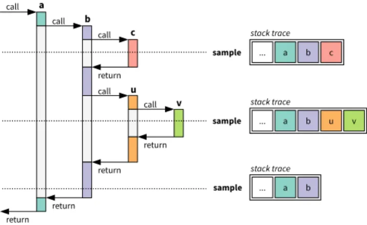
Figure 5: Three samples with complete stack traces

5.

INCREMENTAL STACK TRACING

Self-sampling and partial safepoints reduce the time that an application must pause for sampling. To further lower the overall overhead, we looked at the costs of the stack walk. In many cases, the stack frames from the stack base up to a certain stack depth remain unchanged for most of a thread’s execution. Nevertheless, these unchanged frames are examined during every stack walk.

Figure 5 shows an example for redundantly sampled frames, starting with a call to the methoda. Methodacallsb, which in turn callsc. While execution is inc, the profiler takes a sample. The stack walk visits the frames of the three active methods as well as all frames belowa. When the profiler takes the next sample inv,c has returned, the frame ofb

has changed becausebcontinued its execution, and two new frames from the calls touandvare on the stack. Although the frame ofaand all frames below it remained unchanged, the stack walk needlessly walks and decodes them again. When the profiler takes a third sample, the frames ofuand

vhave disappeared and only the frame ofbhas changed, but the stack walk again visits all other frames as well.

To avoid redundantly sampling frames, stack walks could be limited to a certain number of frames below the frame of the executing method. However, the resulting incomplete stack traces would not be suitable to be correctly merged into a CCT, which has the entry method as its root. Therefore, we devised an approach that builds stack traces incrementally when methods return, and does not examine an unchanged stack frame more than once. We based our technique for incremental stack tracing on an approach that our research group developed for implementing continuations in a Java VM [22]. Similar approaches have also been used to imple-ment increimple-mental scavenging for garbage collection [7].

5.1

Data Structures

To share frame information between stack traces of multiple samples, we store the traces in a tree structure. Figure 6 shows what this tree looks like for the example from Figure 5. We maintain a linked list ofstack trace objectsfor the stack traces that were taken, which is shown on the right-hand side of the figure. Stack trace objects are assigned numeric identifiers, which the profiling agent can use to keep track of the stack traces that it has requested. Each stack trace object has a pointer to aframe objectthat represents the stack frame which was on top of the stack when the stack trace was taken. For the first stack trace, which has the identifier 1, this is

a b c ... u v b'' b' stack traces 1 2 3

Figure 6: Stack traces in a tree with shared frames

the frame object representing the frame forc, for stack trace 2 it is the frame object forv, and for stack trace 3 it is the frame object forb. Each frame object has a pointer to its caller frame object. The frame objectsb,b0andb00refer to the same invocation ofb, but the duplication is necessary because the frame objects store different execution positions (i.e., bytecode indices) within the method. This information is useful to a profiler, for example, to distinguish between different call sites in a method.

Frame objects store the details of a captured stack frame in the following attributes:

parent: The pointer to the caller’s frame object.

method: An identifier of the Java method that the stack

frame belongs to.

bci: The index of the current instruction within the Java bytecode of the method.

The following attributes of a frame object are not intended for the profiler, but are required for capturing frames and managing the tree of frame objects (see the next section).

filled: A value that indicates if the frame object has been

filled with valid data, or if it is an emptyskeleton object.

frame address: The frame’s exact location on the stack.

saved return address: Original return address of the callee.

5.2

Capturing Frames

We maintain one list of stack trace objects for each thread. When we take a new stack trace, we first create a new stack trace object and insert it into the respective thread’s list. We then create a new frame object for the top frame on the stack, which we calltop frame object (TFO). We decode the top frame and fill the TFO with the determined method identifier and bytecode index (see Figure 7 (a)). Theframe address

and thesaved return addressattributes are not required for the TFO. We set the TFO’sfilledattribute and link it with the stack trace object that we created earlier.

In a second step, we deal with the caller frame. The caller frame remains unchanged until the top frame’s method returns, so we do not capture it immediately. Instead, we create askeleton frame objectfor the caller frame that we can fill later, and make this skeleton object the parent of the TFO. We store the caller frame’s address (SPbin Figure 7) in the skeleton object’s frame addressattribute so we can match it to the frame later (see below). To intercept when the top frame’s method returns, we patch the top frame’s return address on the stack with the address of a piece of trampoline code that we generate during the VM’s startup phase. The original return address (RAc in Figure 7) is stored in the skeleton object’ssaved return addressattribute. When the top method returns, it returns to our trampoline instead of to its caller, and the trampoline in turn calls our stack tracing code. In this code, we decode the caller’s frame

filled: yes method: c bci: 42 parent filled: no frame addr: SPb saved ra: RAc Trampoline c RA_c b RAb a RAa ... method: c … parent filled: yes method: b bci: 17 parent

Frame Objects Stack Frame Objects

filled: no frame addr: SPa saved ra: RAb Stack b a ... RA_b RAa Trampoline TFO Skeleton Skeleton (a) (b) SPa SPb

Figure 7: Capturing a frame (a) when taking a sam-ple, and (b) when intercepting a method return

into its skeleton object, patch the caller’s return address on the stack, and create another skeleton object for the caller’s caller frame (see Figure 7 (b)). Finally, we do the actual return by using the saved return address that we stored in the skeleton object before.

To know which frame object must be filled when we in-tercept the return of a method, we maintain a thread-local pointer to the next skeleton object that needs to be filled, which we callcurrent skeleton object (CSO).We also use the CSO to implement sharing of frame objects between multiple stack traces. We distinguish the following situations:

Taking a sample. When we take a sample, we create a

new TFO and fill it with the decoded top frame. Depending on the CSO, the TFO is treated as follows:

• If the CSO is not set yet, we create a new CSO and make it the parent of the TFO.

• If there already is a CSO, we check whether it refers to the frame of the TFO’s caller by comparing their frame addresses. If they match, we make the CSO the parent of the TFO. Otherwise, we create a new CSO and insert it between the TFO and the former CSO.

Intercepting a return. When we intercept a method

re-turn, the CSO always refers to the frame object of the caller, so we decode the caller frame into the CSO. We then inspect the CSO’s parent:

• If there is no parent, we create a new CSO as the parent of the former CSO.

• If the CSO’s parent refers to the frame of the caller’s caller, we make that parent the new CSO.

• If the CSO’s parent refers to some other frame, we create a new CSO and insert it between the former CSO and its parent.

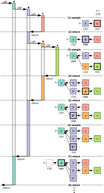
Figure 8 demonstrates how our technique incrementally builds stack traces for the example from Figure 5. Initially, the list of stack traces is empty and there is no CSO. The stack traces are then built in the following steps (for simplicity, we use the name of the methods to also refer to their frames).

(1) To take the first sample, we create a new TFO and decode the top framecinto it (the object that is filled in each step is highlighted in bold). Because there is no CSO yet, we create a skeleton object for the caller

b(skeleton objects are indicated with a dashed frame).

call call call return call call return return return return b c (2) return c a b CSO CSO c a b CSO u v (4) return c a b CSO u v b' (5) return c a b CSO u v b' (6) sample CSO c a b CSO u v b' b'' (7) return c b CSO u v b' b'' ... a (8) return CSO CSO CSO CSO CSO TFO TFO TFO a b c u v (3) sample (1) sample

Figure 8: Incremental construction of stack traces

We make the new skeleton object the CSO and also make it the parent of the TFO. Finally, we patch the return address ofcand save the original return address in the CSO.

(2) Whencreturns, the trampoline is executed, and we fill the CSO with the decoded stack frame ofb. Because the CSO does not have a parent yet, we create a new skeleton object for aas parent. We then make that skeleton object the CSO, patch the return address ofb

and do the actual return fromctob.

(3) When we take the second sample, we decode the top framevinto a new TFO. We then check whether the CSO corresponds to the caller frameu. Since the CSO actually corresponds toa,we create a new CSO foru

and insert it betweenaandv. Finally, we patch the return address ofv.

(4) We intercept the return fromvtouand fill the CSO with the decoded frame ofu. Because the CSO’s parent, which isa,does not matchu’s caller, which isb,we create a new CSOb0 forband insert it betweenaand

u. We finally patch the return address ofuand do the actual return fromvtou.

(5) We intercept the return fromutob and fill the CSO with the decoded frameb. Because the CSO’s parent, which isa,now corresponds tob’s caller, we make the parent the CSO and do not need to create a new one. We also need not patch the return address ofbbecause it was already patched in step (2), and do the actual return fromutob.

(6) When we take a third sample, we fill the top frame

b into a new TFO denoted byb00. Because the CSO corresponds to the caller framea, we make it the parent of the TFO. The return address ofb is still patched and does not need to be modified.

(7) We intercept the return frombtoaand fill the CSO with the decoded framea. Since the CSO does not have a parent here, we create a new CSO fora’s caller. Because all three stack traces join at the frame object ofa,they share this object and all further frame objects below, and we examine their stack frames only once.

5.3

Interface

Typical profiling interfaces, such as JVMTI, offer an oper-ation that walks the stack of a thread and returns a complete stack trace. Our approach does not create such a stack trace right away, but incrementally builds stack traces and requires the profiler to collect them later. Therefore, we devised two operations to use our technique:

sample. The profiler can use thesampleoperation to request a stack trace. It can specify a numeric identifier to assign to the stack trace. The identifiers of stack traces need not be unique, and a profiler can also simply assign timestamps to the stack traces it requests.

retrieve. The profiler can use theretrieveoperation to col-lect all requested stack traces for a set of threads. The stack traces are returned in a tree structure that is similar to the described internal representation. When stack traces are still incomplete, the operation examines the remaining frames on the stack, completes the tree and reverts the patched return addresses on the stack. The retrieve oper-ation empties the tree of stack traces kept in the VM. It always enters a full safepoint, but due to its infrequent use, the introduced overhead is negligible.

We implemented these two operations as JVMTI extension methods, which has the advantage that a profiling agent can probe whether the VM supports incremental stack tracing and partial safepoints. Typically, an agent would period-ically request samples by calling thesamplemethod, and infrequently use the retrieve method to collect the stack traces. It can then merge the stack traces into a calling context tree and update the tree’s edge weights accordingly. The agent must retrieve the samples of a thread before the thread exits, or otherwise the stack traces would be released together with the thread’s resources. It can accomplish this by subscribing to theThreadEndevent that JVMTI offers.

6.

IMPLEMENTATION ASPECTS

When we implemented our techniques in the highly opti-mized HotSpot VM, we had to handle several cases where thread synchronization or taking a correct stack trace is not as straightforward as described in the previous sections.

Frame types. The HotSpot VM starts out by executing

Java bytecode in an interpreter, but compiles frequently executed methods to machine code. Therefore, the stack can contain frames of both interpreted and compiled methods, which differ in their layout. Moreover, Java code can call native methods of the VM, which again use different types of frames. When walking stacks and particularly when patching return addresses, we must handle each type of frame differently.

Inlining. The compiler aggressively tries to inline the code of called methods, and attempts to also inline those methods that are called by the inlined callees. Therefore, a particular location in compiled code can actually lie within multiple in-lined methods that share a single stack frame. The compiler stores information about inlined methods and their ranges within other methods as metadata. When filling the frame object of a compiled frame, we must read this metadata and create extra frame objects for the inlined methods.

Exceptions. When a method throws an exception which

must be handled by a caller, the method does not return in the usual way, using the return address on the stack. Instead, the VM unwinds the stack and pops frames until it reaches a method which can handle the exception. We modified the VM’s exception handling code to capture a frame before it is popped from the stack.

Deoptimization. Deoptimization occurs when a method

was compiled under an assumption that turned out to be false at runtime [15]. An example is when the compiler omit-ted a branch in the compiled code because it assumed that it would never be taken. When deoptimization occurs, the stack frame of the compiled method is transformed into one or more interpreted frames, and execution is continued in the interpreter. During this transformation, patched return addresses are lost, so we had to alter the deoptimization code to preserve patched return addresses.

On-stack replacement. For long-running interpreted

meth-ods, the VM can decide to compile them on the fly, to transform their interpreted frames into compiled frames, and to continue execution in compiled code. This is called on-stack replacement. Since the resulting compiled frames can have different locations than the interpreted frames, we have to update our data structures in this case.

Safepoint synchronization. The safepoint checks that the

HotSpot VM injects into application code simply write a value to a specific page in memory that is calledpolling page.

When no safepoint is pending, these writes are inexpensive. To enter a safepoint, the VM thread acquires the global

threads lockto block thread state transitions, such as when

a thread resumes execution after waiting. Next, the VM instructs the operating system to write-protect the polling page. This causes the safepoint checks to trigger page faults in each thread, and the fault handler then parks the thread. The VM finally waits until all threads are parked or are in a safe state guarded by the threads lock.

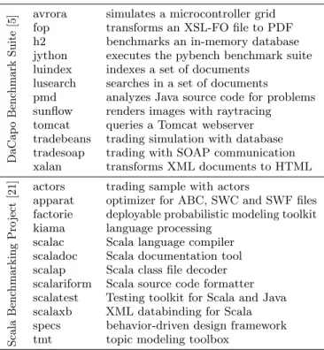
Da Ca p o B en ch m ark S u it e [5

] avrora simulates a microcontroller grid fop transforms an XSL-FO file to PDF h2 benchmarks an in-memory database jython executes the pybench benchmark suite luindex indexes a set of documents

lusearch searches in a set of documents

pmd analyzes Java source code for problems sunflow renders images with raytracing tomcat queries a Tomcat webserver tradebeans trading simulation with database tradesoap trading with SOAP communication xalan transforms XML documents to HTML

S ca la B en ch m a rki n g P ro jec t [2 1 ]

actors trading sample with actors

apparat optimizer for ABC, SWC and SWF files factorie deployable probabilistic modeling toolkit kiama language processing

scalac Scala language compiler scaladoc Scala documentation tool scalap Scala class file decoder scalariform Scala source code formatter scalatest Testing toolkit for Scala and Java scalaxb XML databinding for Scala specs behavior-driven design framework tmt topic modeling toolbox

Table 1: Set of benchmarks

For partial safepoints and self-sampling, we use a modified safepoint mechanism that waits only until enough threads from the desired set of threads have entered the safepoint, and then immediately unprotects the polling page again. However, other threads can also enter the safepoint during that time. Therefore, before write-protecting the polling page, we set a flag for each thread which indicates whether the thread should sample itself. Threads which have their flag set then sample themselves in the fault handler, while the other threads simply wait for the safepoint to end. When including waiting threads for sampling, we compute the ratio of waiting to runnable threads after acquiring the threads lock, so no threads can change their state.

7.

EVALUATION

We evaluated our sampling techniques with the DaCapo 9.12 benchmark suite and the benchmarks of the Scala Bench-marking Project 0.1.0. The DaCapo benchmark suite [5] consists of open source, real-world applications with pre-defined, non-trivial workloads.1 The Scala Benchmarking Project [21] complements the DaCapo suite with a set of benchmarks based on real-world applications written in the Scala language. Table 1 describes the individual benchmarks. We compare the overheads and the generated CCTs of the following techniques relative to no sampling:

• Conventional JVMTI sampling

• Self-sampling in Partial Safepoints (SPS)

• Incremental Self-sampling in Partial Safepoints (ISPS) For that purpose, we implemented two profiling agents that take samples at fixed intervals and build a CCT, one that uses conventional JVMTI, and another one that uses our VM extensions. We enabled sampling of waiting threads

1_{We did not use the DaCapo suite’sbatikandeclipse}

bench-marks because they do not run on OpenJDK 8.

with our techniques to be comparable with JVMTI sampling, which cannot target running threads. We used the number of CPU cores as the number of threads to sample with partial safepoints. Experiments showed that using more threads than that causes considerably more overhead, while using fewer threads does not significantly reduce overhead. The profilers adhere as much as possible to the sampling interval by incorporating the time that elapsed while taking the last sample into the time they wait until taking the next sample. We chose to execute 30 successiveiterationsof each bench-mark with each sampling technique in a single VM instance, and to discard the data from the first 20 iterations to compen-sate for the VM’s startup phase. Hence, our agents track the start and the end of benchmark iterations to extract the met-rics and the generated CCT for every iteration. We further executed 10roundsof each benchmark (with 30 iterations each) to ensure the results are not biased by optimization decisions the VM makes in the warm-up phase.

We performed all tests on a system with a quad-core Intel Core i7-3770 processor with 16 GB of memory running Ubuntu Linux 14.04 LTS. To get more stable results, we disabled hyperthreading, turbo boost and dynamic frequency scaling. With the exception of vital system services, no other applications were running while the benchmarks were executed.

7.1

Overhead

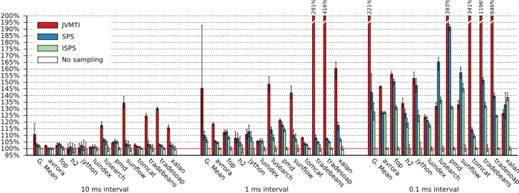
Figure 9 shows the median overheads for the benchmarks of the DaCapo suite with all three sampling techniques, using sampling intervals of 10 ms, 1 ms and 0.1 ms. The error bars indicate the first and third quartiles. TheG.Meanbars show the geometric means for a sampling interval, and their error bars indicate a 50% confidence interval. With 10 ms intervals, JVMTI sampling already has a considerable overhead of more than 10% on average, while that of SPS stays below 3%, and ISPS comes close to 2%. Our techniques have the most impact for thelusearch, sunflow, tradebeans, tradesoapand

xalanbenchmarks. We found that these benchmarks have

a higher CPU usage or use a larger number of threads than the other benchmarks. In comparison, our techniques have little effect for thejythonandluindexbenchmarks, which are mostly single-threaded. Overall, ISPS achieves significantly lower overheads than SPS. Surprisingly, the overhead of JVMTI sampling for lusearch, sunflowand xalan is lower with 0.1 ms sampling intervals than with 1 ms intervals. This can be explained with the sampling latency, which we examine below.

Figure 10 shows the overheads for the benchmarks of the Scala Benchmarking Project. In contrast to the DaCapo benchmarks, even JVMTI sampling has only 5% overhead with 10 ms sampling intervals. The improvements from our techniques become more significant with 1 ms intervals, where JVMTI sampling has approximately 25% overhead while ISPS achieves less than 10% overhead. One interesting case istmt,where ISPS has more overhead than SPS with 10 ms and 1 ms intervals. The reason is thattmtcreates a large number of short-lived threads, and the agent must retrieve the samples of each of those threads when they end. The extra effort for this is typically low, but becomes significant in this case. We were unable to measure the overhead of

actorswith JVMTI sampling with 0.1 ms intervals because

that benchmark has an internal timeout which causes it to terminate early due to the high overhead.

95% 100% 105% 110% 115% 120% 125% 130% 135% 140% 145% 150% 155% 160% 165% 170% 175% 180% 185% 190% 195% 200% G. Mea n

avrorafop h2 jythonluindexlusearchpmdsun fl_ow tomcattradebe ans tradeso ap xalan G. Mea n

avrorafop h2 jythonluindexlusearchpmdsun fl_ow tomcattradebe ans tradeso ap xalan G. Mea n

avrorafop h2 jythonluindexlusearchpmdsun fl_ow tomcattradebe ans tradeso ap xalan JVMTI SPS ISPS No sampling 291% 416% 221% 393% 341% 1196% 646% 0.1 ms interval 1 ms interval 10 ms interval

Figure 9: Overhead with the DaCapo benchmark suite using sampling intervals of 10ms, 1ms and 0.1ms

95% 100% 105% 110% 115% 120% 125% 130% 135% 140% 145% 150% 155% 160% 165% 170% 175% 180% 185% 190% 195% 200% G. Mea n actorsappara t factoriekiamascalacscalado c scalapscalarif orm scalate st

scalaxbspecstmt G. Mea n actorsappara t factoriekiamascalacscalado c scalapscalarif orm scalate st

scalaxbspecstmt G. Mea n actorsappara t factoriekiamascalacscalado c scalapscalarif orm scalate st scalaxbspecstmt JVMTI SPS ISPS No sampling 225% 402% 359% 295% 255% 225% 201% 213% 0.1 ms interval 1 ms interval 10 ms interval

Figure 10: Overhead with the benchmarks of the Scala Benchmarking Project

7.2

Latency

We examined the latency of each sampling technique, which is the time it takes to pause threads and take samples. Fig-ure 11 shows box plots of the latencies for all sampling tech-niques with 1 ms sampling intervals. The whiskers indicate the 2.5% and 97.5% percentiles. We grouped benchmarks with similar characteristics inOthers. For all those bench-marks, the latency of JVMTI sampling is low, and SPS and ISPS have slightly lower latencies. For the other shown benchmarks, we found notable differences.actors, tradebeans

andtradesoapuse a large number of threads and the median

latency with JVMTI sampling is high because it takes longer until all threads have entered a safepoint. The latency with SPS and ISPS is not higher than for all the other benchmarks because these techniques only require some of the threads to enter a safepoint. lusearch, sunflowandxalanhave fewer threads, but they are very CPU-intensive and the compiler aggressively optimizes the hot code and eliminates safepoint checks. While the median latency for those three benchmarks with JVMTI sampling is not excessively high, the latencies fluctuate significantly between samples and can reach more

than 10 ms, which results in fewer taken samples. We found that with CPU-intensive benchmarks, such excessively high latencies occur more often when using shorter sampling inter-vals, possibly due to scheduling effects. A shorter sampling interval can then yield fewer total samples than a longer interval and actually reduce the overhead compared to a longer interval. This was the case with our overhead mea-surements with 0.1 ms intervals for those three benchmarks. In comparison, the latency with SPS and ISPS for these benchmarks is not higher than for the other benchmarks and very stable.

7.3

Accuracy

Determining the absolute accuracy of a profiler is chal-lenging: ideally, we would compare a CCT from the profiler against an exact CCT of the same execution. However, such a perfect profile cannot be obtained because all profiling has an effect on the profiled application. While instrumenting profilers can generate a complete CCT with exact call counts, instrumentation significantly slows down short-running meth-ods and interferes with compiler optimizations (particularly

0.0 ms 0.2 ms 0.4 ms 0.6 ms 0.8 ms 1.0 ms 1.2 ms 1.4 ms 1.6 ms Other s actors tradeb eans trades oap lusear ch sun fl_ow xalan JVMTI SPS ISPS

Figure 11: Pause times for selected benchmarks

inlining). Therefore, when using instrumentation to measure execution times, the measured times are not representative for the unaltered application. Instead, we analyze whether each sampling profiler generates similar CCTs for different iterations of the same benchmark. We further construct “averaged” CCTs from different iterations of each benchmark with each profiler and compare them to test whether the profilers agree.

To compare two CCTs with each other, we use thedegree of

overlapandhot-edge coveragemetrics. The degree of overlap

assesses how many edges of the two CCTs are equivalent and how close their edge weights are to each other. It has been described and used extensively in related research [8, 9, 12, 16, 25]. While the degree of overlap reflects all edges of the two CCTs, the hottest edges of a CCT are of particular interest for identifying performance bottlenecks. The hot-edge coverage metric determines whether two CCTs identify a similar set of edges as hot according to a relative threshold and puts less emphasis on the exact edge weights. It was introduced in [25] and is used in [8, 12].

For the results we present below, we used the CCTs that we collected with a sampling interval of 1 ms. However, we found that the results are similar for sampling intervals of 10 ms and 0.1 ms. For each sampling technique and benchmark, we merged the CCTs from every (undiscarded) iteration in all rounds into a single CCT. This merged CCT contains all edges that exist in any of the CCTs, with edge weights that are the sum of the relative edge weights from all CCTs. The merged CCT is thus really the average over all individual CCTs of a benchmark. Some of the benchmarks dynamically generate classes which can be assigned different names in different iterations or rounds, for example call wrappers or web service handlers. We added extra heuristics to our analysis tools to properly match identical generated code when merging CCTs.

Stability Analysis.

The behavior of most benchmarks does not deviate much between iterations and thus, a profiler should produce similar CCTs for different iterations. We determined the stability of the CCTs of a profiler by comparing the CCT of every iteration to the average CCT of each benchmark.

0% 10% 20% 30% 40% 50% 60% 70% 80% 90% 100% Overlap 0% 10% 20% 30% 40% 50% 60% 70% 80% 90% 100%

avrorafop h2 jythonluindexlusearchpmdsun

fl_ow tomcattradebe ans tradeso ap xalanactorsappara t factoriekiamascalacscalado c scalapscalarif orm scalate st scalaxbspecstmt Hot-Edg e Cover age JVMTI SPS ISPS

Figure 12: Overlap (top) and hot-edge coverage

(bottom) of individual CCTs with average CCT

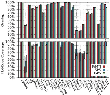
Figure 12 shows the similarity of the individual CCTs with the average CCT by means of their median overlap (top part) and their median hot-edge coverage (bottom part), for all benchmarks and all profiling techniques. We used a threshold ofT = 0.1 for the hot-edge coverage, which means that we consider an edge to be hot if it is within a tenth of the hottest edge. The error bars indicate the first and third quartiles. The plots demonstrate that for every benchmark, the stability of all three sampling techniques is very similar. They also suggest that the behavior offop, kiama, scalac,

scaladocandscalaxbvaries significantly between iterations.

We found that these benchmarks spend over 40% of their execution time in many different calling contexts, each of which making up less than 0.05% of the overall execution time, in many cases even less than 0.01%. Hence, these calling contexts are seen in only very few samples and even slight shifts in sampling times add up to a significant difference in the resulting overlap. The hot-edge coverage for these benchmarks is significantly better, with the exception offop:

it has the shortest execution time of all benchmarks, so the profiler collects the fewest samples, and since it does not have any significantly hot calling contexts, the relative threshold causes a large set of calling contexts to be considered hot.

Our results show that all three sampling techniques pro-duce CCTs that are stable between different iterations of most benchmarks. At the same time, the results demonstrate that the average CCTs are representative for the individual CCTs. However, this does not prove that the CCTs are accu-rate, since a sampling technique can also repeatedly produce an incorrect CCT.

Comparison between Sampling Techniques.

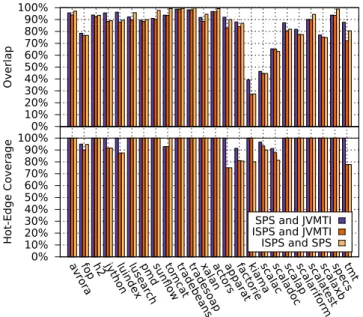
Figure 13 compares the average CCTs obtained with the three sampling techniques to each other by means of their overlap (top part) and their hot-edge coverage with a thresh-old of T = 0.1 (bottom part). The overlap between the three profiling techniques exceeds 70% for all benchmarks, with the exception ofkiama, scalac andscaladoc. These

0% 10% 20% 30% 40% 50% 60% 70% 80% 90% 100% Overlap 0% 10% 20% 30% 40% 50% 60% 70% 80% 90% 100%

avrorafop h2 jythonluindexlusearchpmdsun fl_ow tomcattradebe ans tradeso ap xalanactorsappara t factoriekiamascalacscalado c scalapscalarif orm scalate st scalaxbspecstmt Hot-Edg e Cover age SPS and JVMTI ISPS and JVMTI ISPS and SPS

Figure 13: Overlap (top) and hot-edge coverage

(bottom) of average CCTs from different sampling techniques

three benchmarks implement recursive-descent parsers with very deep stacks, and their rapidly changing stack depths make it improbable that many calling contexts are captured more than once. The hot-edge coverage plots show that SPS identifies a similar set of hot calling contexts as JVMTI sampling, with over 90% coverage for all benchmarks. We conclude from this that partial safepoints have no negative effect on the accuracy in comparison to sampling all threads. The hot-edge coverage between ISPS and the other two tech-niques is slightly lower for some benchmarks. The reason are deep stacks which exceed the otherwise adequate limit of 256 frames that we use for SPS and JVMTI sampling. Such a limit is required for the preallocation of data structures and we found that using a limit that is high enough to fit every stack trace significantly increases the overhead even for shallow stacks. While SPS and JVMTI sampling truncate long stack traces, ISPS always provides complete stack traces. While this is actually an advantage of ISPS, it reduces its hot-edge coverage with the other techniques because the complete stack traces do not match their truncated stack traces.

8.

RELATED WORK

In this section, we describe previous work on profiling Java applications, on sampling calling context for dynamic analysis, and on analyzing CCTs.

Profiling.

Whaley [24] describes a VM-internal Java profiler which avoids complete stack walks. Unlike incremental stack trac-ing, it examines stacks eagerly and uses a spare bit in each stack frame’s return address to mark if a frame has already been examined. Whaley claims a low overhead of 2-4% at 1000 samples per second, but the used VM performs thread scheduling itself (“green threads”), which permits certain as-sumptions and direct access to thread states. Green threads are uncommon in modern Java VMs because of their

disad-vantages in systems with multiple CPUs. Our techniques have only slightly more overhead with the high-performance HotSpot VM and work well for multi-processor systems.

Zhuang et al. [25] describe a Java profiler that does not sample stack traces, but instead instruments the code to sample sequences (“bursts”) of calls and returns, and uses heuristics to disable and re-enable sampling to reduce redun-dant samples. The resulting CCTs are claimed to have more than 80% hot-edge coverage and overlap with exhaustive CCTs, but the stated overhead of 20% for 10 ms sampling intervals is significantly higher than that of our techniques. Binder [4] presents a Java profiler that instruments meth-ods to maintain a shadow method stack and to periodically capture samples of this stack, which he claims is more ac-curate than JVMTI sampling. Unlike our techniques, this profiler can be implemented in pure Java, but its overhead is much higher and comparable to that of JVMTI sampling. Inoue and Nakatani [14] describe a Java profiler that uses hardware events to take samples of only the executing method and its stack depth. It builds a CCT through matching stack depths and caller information, and is reported to achieve an overhead of 2.2% at 16000 samples per second. Similarly, Serrano et al. [20] present a Java profiler that uses hardware branch tracing to create partial call traces and attempt to merge them optimally into approximate CCTs, claiming to produce highly accurate CCTs at negligible overhead. Unlike our techniques, both of these techniques require specific hardware and their accuracy can suffer from caller ambiguity.

Dynamic analysis.

Calling context information is also useful for locating data races, memory leaks and other anomalies with dynamic anal-ysis tools. Such tools capture the calling context frequently enough so that continuously maintaining the current calling context is often faster than walking the stack for each sam-ple. Bond and McKinley [6] describe an approach in which they instrument code so that it continuously maintains a probabilistically unique number for the current calling con-text. This number is then sampled at certain points, such as calls to library methods. A dynamic analysis tool can then compare traces of these samples between executions of a program for anomaly detection. They claim that their ap-proach has an overhead of 3% for such applications. Sumner et al. [23] describe a similar approach for encoding the calling context as a number and report an overhead of 2%. Huang and Bond [13] claim that the accuracy of such approaches does not scale well with program complexity and propose an approach that continuously builds a CCT-like data struc-ture through instrumentation. It creates tree nodes eagerly and relies on a modified garbage collector to release unused nodes and to merge duplicate nodes. Using this technique to add calling context information to a memory leak detector or to a data race detector is claimed to introduce around 30-40% extra overhead. We believe that incremental stack tracing can achieve equivalent or less overhead than these techniques because it also does not walk the stack for each sample, but does not introduce overhead in methods where calling contexts are not needed.

Profile analysis.

The calling context trees of real-world applications can be very large and complex so that it can be difficult to identify performance bottlenecks in them. Moret et al. [17] as well

as Adamoli and Hauswirth [1] describe approaches for visu-alizing and analyzing large and complex CCTs. D’Elia et al. [8] describe algorithms to continuously maintain a “Hot CCT” that includes only hot calling contexts. They claim that it is orders of magnitudes smaller than a regular CCT at comparable accuracy. These algorithms could be used with our sampling techniques to build a memory-efficient profiler. The low overheads of our techniques also make it feasible to enable them in an end-user product or in production systems to gather performance data for real-world usage. Han et al. [10] describe an approach to identify performance prob-lems through pattern mining in vast amounts of performance data, which could be used to analyze data collected this way.

9.

CONCLUSIONS AND FUTURE WORK

With partial safepoints, self-sampling and incremental stack tracing, we presented three novel techniques that re-duce the overhead of sampling Java applications and allow a profiler to target just the running threads. Unlike many other fast profiling approaches, our techniques require no support from the operating system or from hardware. Ex-periments with our implementation in the HotSpot Java VM demonstrate that these techniques significantly reduce the sampling overhead while providing high accuracy.

In the future, we intend to look at improvements to the accuracy of Java profiling techniques. For example, when the JIT compiler eliminates safepoint checks to optimize hot code regions, it prevents profilers from taking samples in these regions, which can severely distort the profile of some programs. We consider introducing light-weight “sam-pling points” which make fewer guarantees about safety than safepoints and therefore do not obstruct compiler optimiza-tions. Instead of eliminating a safepoint check, the JIT compiler could downgrade it to a sampling point check and still produce fast code. We have also experimented with us-ing facilities of the operatus-ing system, such as POSIX signals, to interrupt individual threads for sampling with incremental stack tracing. However, patching return addresses on the stack is much more difficult and error-prone when a thread is not in a safepoint, and a correct implementation requires substantial modifications to the VM. Finally, we consider extending incremental stack tracing to track the values of variables. This should be possible at less runtime and space overhead than with exhaustive stack tracing and would be particularly valuable as input for profile-guided optimization.

10.

ACKNOWLEDGEMENTS

This work was supported by the Christian Doppler For-schungsgesellschaft, and by Compuware Austria GmbH.

11.

REFERENCES

[1] A. Adamoli and M. Hauswirth. Trevis: A context tree visualization & analysis framework and its use for classifying performance failure reports. SOFTVIS ’10, pages 73–82. ACM, 2010.

[2] G. Ammons et al. Exploiting hardware performance counters with flow and context sensitive profiling. PLDI ’97, pages 85–96. ACM, 1997.

[3] M. Arnold and D. Grove. Collecting and exploiting high-accuracy call graph profiles in virtual machines. CGO ’05, pages 51–62. IEEE, 2005.

[4] W. Binder. Portable and accurate sampling profiling for Java.Software: Practice and Experience, 36(6):615–650, May 2006.

[5] S. M. Blackburn et al. The DaCapo benchmarks: Java benchmarking development and analysis. OOPSLA ’06, pages 169–190. ACM, Oct. 2006.

[6] M. D. Bond and K. S. McKinley. Probabilistic calling context. OOPSLA ’07, pages 97–112. ACM, 2007. [7] A. M. Cheadle et al. Non-stop Haskell.SIGPLAN

Notices, 35(9):257–267, Sept. 2000.

[8] D. C. D’Elia et al. Mining hot calling contexts in small space. PLDI ’11, pages 516–527. ACM, 2011.

[9] P. T. Feller. Value profiling for instructions and memory locations. Master’s thesis, UC San Diego, 1998. [10] S. Han et al. Performance debugging in the large via

mining millions of stack traces. ICSE ’12, pages 145–155. IEEE, 2012.

[11] P. Hofer and H. M¨ossenb¨ock. Efficient and accurate stack trace sampling in the Java Hotspot virtual machine. ICPE ’14, pages 277–280. ACM, 2014. [12] P. Hofer and H. M¨ossenb¨ock. Fast Java profiling with

scheduling-aware stack fragment sampling and asynchronous analysis. PPPJ ’14, 2014. To appear. [13] J. Huang and M. D. Bond. Efficient context sensitivity

for dynamic analyses via calling context uptrees and customized memory management. OOPSLA ’13, pages 53–72. ACM, 2013.

[14] H. Inoue and T. Nakatani. How a Java VM can get more from a hardware performance monitor. OOPSLA ’09, pages 137–154. ACM, 2009.

[15] T. Kotzmann et al. Design of the Java HotSpotTM

client compiler for Java 6.ACM Transactions on

Architecture and Code Optimization, 5(1):7, 2008.

[16] P. Moret et al. CCCP: complete calling context profiling in virtual execution environments. PEPM ’09, pages 151–160. ACM, 2009.

[17] P. Moret et al. Exploring large profiles with calling context ring charts. WOSP/SIPEW ’10, pages 63–68. ACM, 2010.

[18] Oracle. JVMTM_{Tool Interface version 1.2.1.}

http://docs.oracle.com/javase/7/docs/platform/ jvmti/jvmti.html.

[19] Oracle. OpenJDK HotSpot group.

http://openjdk.java.net/groups/hotspot/. [20] M. Serrano and X. Zhuang. Building approximate

calling context from partial call traces. CGO ’09, pages 221–230. IEEE, 2009.

[21] A. Sewe et al. Da Capo con Scala: design and analysis of a Scala benchmark suite for the Java virtual machine. OOPSLA ’11, pages 657–676. ACM, 2011. [22] L. Stadler et al. Lazy continuations for Java virtual

machines. PPPJ ’09, pages 143–152. ACM, 2009. [23] W. N. Sumner et al. Precise calling context encoding.

IEEE Trans. Softw. Eng., 38(5):1160–1177, Sept. 2012.

[24] J. Whaley. A portable sampling-based profiler for Java virtual machines. JAVA ’00, pages 78–87. ACM, 2000. [25] X. Zhuang et al. Accurate, efficient, and adaptive

calling context profiling. PLDI ’06, pages 263–271. ACM, 2006.