Using holistic features for scene classification by combining classifiers

(1)

Using holistic features for scene classification by

combining classifiers

Kelly Assis de Souza Gazolli Universidade Federal do Espírito Santo

Evandro Ottoni Teattini Salles Universidade Federal do Espírito Santo

ABSTRACT

Scene classification is a useful, yet challenging problem in computer vision. Two important tasks for scene classification are the image representation and the choice of the classifier used for decision making. This paper proposes a new technique for scene classification using combined classifiers method. We run two classifiers based on different features: GistCMCT and spatial MCT and combine the output results to obtain the final class. In this way, we improve accuracy, by taking advantage from the qualities of the two descriptors, without increasing the final size of the feature vector. Experimental results on four used datasets demonstrate that the proposed methods could achieve competitive performance against previous methods.

Keywords

visual descriptor, gist, CMCT, CENTRIST, combining classifiers.

1. INTRODUCTION

The scene classification is an important topic in computer vision. However, while classifying a scene is not a problem for humans, it is quite a challenging task for computers. Among the reasons is the significant intra-class variations, since a scene is composed of several entities often organized in an unpredictable layout. Moreover, there are other obstacles such as, variations in lighting and scale, different view angles, occlusion and dynamic backgrounds. All these factors make it difficult to find a unique representation for a scene category that encompasses all possible variations for scenes belonging to it. The holistic approach is a common method for scene classification. This approach does not require explicit segmentation of image and objects, the image is considered as a whole. Oliva and Torralba [Oli05a][Oli01a] showed that scenes which belong to the same category, normally, have the same spatial layout properties (naturalness, openness, expansion, depth, roughness, complexity,

ruggedness, symmetry) and proposed a holistic approach to build the ''gist'' of the scene. Wu and Rehg [Wu11a] also used a holistic approach and proposed CENTRIST (Census Transform Histogram), a representation that captures structural properties, such as, rough geometry and generalizability, by modeling distribution of local structures. In this sense, a modification of CENTRIST was proposed, the CMCT (Contextual Mean Census Transform) [Gaz12a]. In this representation the modeling of distribution of local structures is combined with contextual information. Another approach used in scene classification is the spatial pyramid representation [Lab06a] that captures useful information, like regularities in the image and spatial arrangement of the features, in order to improve the classification task. Wu and Rehg, in [Wu11a], proposed the spatial PACT (Principal component Analysis of Census Transform histograms) a technique which combines spatial information with CENTRIST and improve the classification performance.

In this paper, we work with two different features: GistCMCT [Gaz13a] and spatial MCT. GistCMCT combines the vector generated from gist [Oli01a] [Oli06a] with the vector generated from CMCT [Gaz12a] in a new vector with the aim of improve classification results as much as for indoor as for outdoor scenes. In the other hand, spatial MCT uses

Permission to make digital or hard copies of all or part of this work for personal or classroom use is granted without fee provided that copies are not made or distributed for profit or commercial advantage and that copies bear this notice and the full citation on the first page. To copy otherwise, or republish, to post on servers or to redistribute to lists, requires prior specific permission and/or a fee.

(2)

2. THEORETICAL

BACKGROUND

2.1 Modified Census Transform

The Modified Census transform (MCT) [Fro04a] is inspired on Census Transform [Zab94a], a nonparametric local transform originally designed for computing visual correspondence, and it was proposed by Fröba and Ernst with the aim of overcome some weakness of Census Transform. First, The Modified Census Transform, Г(x), computes a mean Ix over 3 x 3 window of pixels. So, every pixel in the 3 x 3 window is then compared with Ix. If the pixel is bigger than or equal to Ix, a bit 1 is set in the corresponding location, otherwise, a bit 0 is set, as follows

 x= 

y∈N 'xIy,Ix,

m ,n=1,mn ; m , n=0,otherwise

where



represents concatenation operation, Ix is the mean of the intensity values in the 3 x 3 window of pixels centered at x, I(y) is the gray value of the pixel at y position and N'(x) is a local spatial neighborhood of the pixel at x so that

Nx=N 'x∪x. In the Modified Census Transform technique, 9 bits are generated and converted to a decimal number in [0, 511], namely, here, MCT.

2.2 CMCT - Contextual Mean Census

Transform

Contextual information provides a support for scene classification. A white image region is likely to be the cloud if it is in a sky area while could be snow if it is next to a mountain. With the aim of adding contextual information to MCT descriptor, Gazolli and Salles [Gaz12a] proposed the Contextual Mean Census Transform (CMCT), which integrates contextual information with local structures information for differentiating windows in the image that have similar structures, but have significant difference in their neighborhood. For accomplishing this task, this approach considers information from

Transform with 8 bits this last is referred as MCT8.

The steps for the Contextual Mean Census Transform (CMCT) generation are as follow. First, MCT8 is computed for all pixels. Then, a histogram of MCT8 is obtained. A new image is created in which the original image pixels are replaced by the correspondent MCT8 values as shown in Fig. 1. In the sequel, the MCT8 is computed on the new image pixels and a new histogram is generated. Then, the MCT8 histogram for the original image histogram and the the MCT8 histogram for the new image are concatenated, generating a new descriptor. The whole process is schematized in Fig. 2.

2.3 GistCMCT

Under the assumption that is not necessary identify the objects that make up a scene to identify the scene, Oliva and Torralba [Oli01a] proposed a holistic approach to build the 'gist' of the scene using a low-dimensional representation of perceptual dimensions, a set of global image properties, such as naturalness, openness, roughness, expansion and ruggedness. This approach uses those perceptual dimensions to define the functionality of the scene location in the three-dimensional space. The set of perceptual dimensions is named Spatial Envelope. As gist is a holistic representation of the scene structure, it does not require explicit segmentation of image and objects.

Figure 1. Pixel value is replaced by the MCT8 for obtaining contextual information.

(3)

Gist represents the shape of the scene by computing stable spatial structures within images that reflect functionality of the location. Besides that, gist has a certain weakness in recognizing indoor scenes, but is quite efficient in the recognition of outdoor scenes [Wu11a]. In the other hand, CMCT summarizes local shape information. This descriptor represents structural properties through the distribution of local structures (for example, the amount of local structures that are local horizontal edge) [Wu11a] which helps in the classification of man-made environments, including, indoor environments. Aiming the improvement of classification results as much as for indoor as for outdoor scenes, the GistCMCT [Gaz13a] was proposed. The GistCMCT combines the vector generated by gist [Oli01a] [Oli06a] with the vector generated by CMCT [Gaz12a] in a new one vector. The new vector gathers qualities from gist and CMCT, reaching, hence, a better performance in classifying scenes. The information about the perceptual dimensions can be extracted from linear filters [Oli05a]. In this work, the gist descriptor was obtained from a bank of Gabor filters. We used 4 scales and 8 orientations and the outputs of the filters were downsampled in a 4 x 4 grid, generating a vector with 512 positions. As CMCT also generates a 512 size vector, the final descriptor is a vector with 1,024 positions.

2.4 Spatial Information

Lazebnik el al. showed in [Lab06a] that the spatial arrangement of the features and the regularities in image composition provides powerful cues for scene classification tasks. In order to incorporate spatial information, Wu and Rehg [Wu11a] proposed a spatial representation which is based on the Spatial Pyramid Matching scheme in [Lab06a]. In this

representation, the image is divided in blocks and the correspondent results in these blocks are concatenated. However, in order to avoid artifacts created by the non-overlapping division, the blocks division is shifted. Besides that, the image is resized between different levels so that all blocks contain the same number of pixels.

In this work, we adopted the representation proposed in [Wu11a]. However, instead of using CENTRIST, we apply MCT [Fro04a], once by using MCT it is possible differentiating structures that are considered equal by CENTRIST. The MCT vectors obtained in all blocks are then concatenated to form an overall feature vector. After obtaining the final vector, we used Principal Component Analysis to reduce its dimensionality, in the same way as [Wu11a]. We use 3 levels of spatial information, as [Wu11a], which generates 31 blocks and reduce the dimensionality of each block from 512 to 40. We also adopted the extra information (mean and standard deviation of pixel blocks). We refer the spatial pyramid of MCT as spatial MCT.

3. ADDING SPATIAL

INFORMATION BY COMBINING

CLASSIFIERS

As we presented in Section 2.3, GistCMCT combines two different feature descriptors in order to improve both indoor and outdoor scene classification. However, GistCMCT does not consider the spatial layout of the features in image. Spatial MCT, on the other hand, does, and, as discussed in Section 2.4, this type of information can help improving the classification results.

According to [Ho94a], the classification accuracy could be improved by using features and classifiers of

(4)

sets trains an individual classifier and the results of these classifiers are used for decision making by combining their individual opinions to derive a consensus decision.

The classifier adopted for both descriptors is the SVM (Support Vector Machine), a pattern classifier introduced by Vapnik [Vap98a], with Histogram Intersection kernel (HIK) [Wu09a]. Despite of using the same type of classifier, the features extracted from the images are unique to each one, since each classifier uses its own representation of the image (GistCMCT or spatial MCT). In this way, we integrate physically different types of features. The implementation of a multiple classifier system implies the definition of a rule (combining rule) for determining the most likely class, on the basis of the class attributed by each single classifier [Fog07a]. For combining the individual opinion from each classifier, we used the combination rules Max, Median and Product presented in [Kit98a]. For simplicity, we assume that the results from each classifier are statistically independent. For equiprobable distribution classes, the selected  class is the one that satisfies to the following equations [Kit98a]  Max: max_iR₌₁_P_ j∣xi=maxk=1 m _max i=1 R _P_ k∣xi  Median med_iR₌₁_P_ j∣xi=maxk=1 m _med i=1 R _P_ k∣xi  Product:

∏

i=1 R P_j∣xi=maxk=1 m

∏

i=1 R P_k∣xi

where m is the number of possibles classes 1,...,m, xi is the measurement vector used by the

ith classifier, and R is the number of classifiers, in our case, R=2.

4. EXPERIMENTS

In this section, we investigate the effectiveness of our representations and compare them with existing works.

(356 images) and street (292 images). The size of each image is 256 x 256.

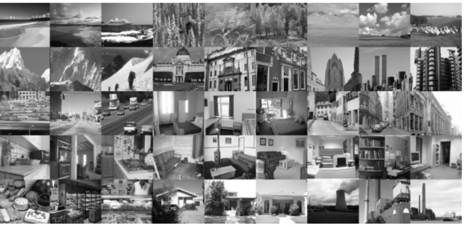
 15-category dataset [Lab06a], which is an extension of dataset described above by adding 7 new scene categories: bedroom (216 images), kitchen (210 images), living room (289 images), office (215 images), suburb (241 images), industrial (311 images) and store (315 images). This dataset contains 4,486 gray-values images in total. The image size is approximately 300 x 250. Fig. 3 depicts the samples from this dataset

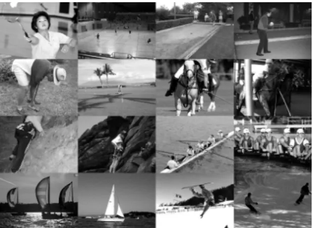
 8-class sports event [Li07a]. This dataset contains 1,579 images of eight sports: badminton, bocce, croquet, polo, rock climbing, rowing, sailing and snowboarding. The number of images in each category varies from 137 to 250. Fig. 4 depicts the samples from this dataset.

 67-class indoor scene recognition [Qua09a]. This dataset contains 15,620 images. The scenes varies from corridor to bakery. This dataset poses a challenging classification problem [Qua09a].

In the experiment, each dataset category is split randomly into a training set and a test set. The random splitting is repeated 5 times, and the average accuracy is reported, as adopted by [Wu11a]. All color images were converted to gray scale. For

Figure 4. Two images from each 8 sports events categories. The categories are: badminton, bocce,

croquet, polo, rock climbing, rowing,sailing and snowboarding (from top to bottom and left to

(5)

training and classification, we adopted SVM (Support Vector Machine) and used the libSVM [Cha11a] package modified by [Wu09a], which offers the option of choose the estimated multi-class probability as output [Wu04a].

Besides that in all experiments performed, we employed Histogram Intersection kernel (HIK) [Wu09a] Support Vector Machine, because the best results were achieved when using this kernel type. For testing gist we used the Lear's gist implementation1_.

4.2 Results on 15-category Dataset

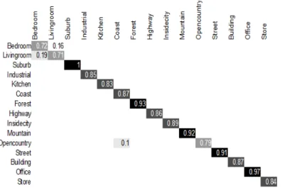
In this dataset an amount of 100 images in each category are used for training and the remaining images constitute the testing set, as in previous researches. When using our approach with product rule, we achieve 86.25 ± 0.51% accuracy in this dataset. Fig. 5 presents the confusion matrix from one run on 15-class scene dataset. We observe that the highest recognition rate was achieved for suburb class. The biggest confusion happens between bedroom and living room, which have similar elements. Humans may confuse them due to the small inter-class variation.

Table 1 presents the classification performance of the proposed method on 15-category dataset compared with existing methods in literature. All approaches in this section used the SVM classifier.

In [Lab06a], it is proposed the spatial pyramid method (SPM), a extension of an orderless bag-of-features image representation. The best performance of SPM is achieved with vocabulary size = 400 and level number = 3 (with leads to a 34000 dimensions final vector). Ergul and Arica [Erg10a] proposed a scene classification method which combines two popular approaches in the literature: Spatial Pyramid

1 _{Available in http://lear.inrialpes.fr/software}

Matching (SPM) and probabilistic Latent Semantic Analysis (pLSA) modeling, the Cascaded pLSA. The results presented here refers to a 5900 dimensions vector.

Method Accuracy(%)

SPM [Lab06a] 81.4 ± 0.5 Cascaded pLSA [Erg10a] 83.31 CENTRIST (3 levels) [Wu11a] 83.88 ±0.76 LDBP [Men12a] 84.10 ± 0.96 CBoW_SL [Li11a] 85.1 LBP + Semantic [Li11b] 85.1

GistCMCT [Gaz13a] 82.72 ± 0.55 Spatial MCT 84.47 ± 0.63

Ours (rule: max) 86.02 ± 0.46

Ours (rule: median) 86.30 ± 0.62

Ours (rule: product) 86.25 ± 0.51 Table 1. Comparison classification results for 15

categories with existent works.

In [Wu11a] the CENTRIST with 3 levels, 40 eigenvectors and 1302 dimensions reached the best result. In [Men12a], the histogram of local transform represents a scene images. This histogram is an extended version of census transform histogram, by applying Local Difference Binary Pattern (LDBP). Besides that, this approach also uses a spatial pyramid representation. In this approach, the final descriptor has 840 dimensions. In [Li11a] a novel contextual Bag-of-Words (CBoW) representation was proposed to model two kinds of typical contextual relations between local patches: a semantic conceptual relation and a spatial neighboring relation. The best performance is achieved when the proposed CBoW is combined with the spatial layout (CboW_SL), with leads to a 2250 dimensions vector. Li and Dewen [Li11b] proposed a

Figure 3. Three images from each 15 scene categories. Thecategories are: coast, forest, open country, mountain, inside city, tall building, highway,bedroom, street, kitchen, living room, office, store, suburb and

(6)

scene classification approach based on combining low-level, by using Local Binary Pattern (LBP), and semantic modeling strategies, local feature extraction and codebook generation. The codebook size was not informed.

As one can see, the proposed approach reached better results than the above methods, including GistCMCT and Spatial MCT separately. With respect to the three combining rules here used, the results were close, despite the max rule achieved the worst result.

4.3 Results on 8-category Dataset

In this dataset an amount of 100 images in each category are used for training and the remaining images constitute the testing set, as in previous researches. In the 8-category scene class our method, with product rule, achieves 88.95 ± 0.49% accuracy. Table 2 shows experimental results for 8-category dataset. As one can see, the proposed method overcomes all aforementioned methods.

Method Accuracy (%)

Gist [Oli01a] 82.60 ± 0.86 Novel Gist [Men10a] 86.60 ± 0.53 CENTRIST (3 levels) [Wu11a] 86.20 ± 1.02 GistCMCT [Gaz13a] 85.82 ± 0.93 Spatial MCT 87.65 ± 0.24

Ours (rule: max) 88.51 ± 0.33

Ours (rule: median) 88.83 ± 0.46 Ours (rule: product) 88.95 ± 0.49

Table 2. Experimental results for 8 scene categories dataset.

The Novel Gist [Men10a] is an extension of census transform and also uses spatial information. In this technique the histograms of upper pattern and lower pattern are computed and then concatenated. The

experiments reported uses SMV classifier and a 1610 dimensions vector.

Once again, the proposed approach reached better results than GistCMCT and Spatial MCT separately. With respect to combining rule, the results were close, but, as in the 15 scene datasets, the max rule reached the worst result.

4.4 Results on 8-class Sports Event

Following [Li07a], in this dataset, we use 70 images per class for training and 60 for testing. Table 3 shows the results for this dataset.

Scene + object [Li07a] 73.4 CENTRIST (3 levels) [Wu11a] 78.25 ± 1.27 GistCMCT [Gaz13a] 74.37 ± 1.34 Spatial MCT 80.63 ± 1.17

Ours (rule: max) 80.96 ± 0.86

Ours (rule: median) 81.33 ± 1.19

Ours (rule: product) 81.54 ± 1.62 Table 3. Experimental results for 8 class sports

event dataset.

In [Li07a], in which the event classification is a result of scene environment classification, object categorization, a manual segmentation and finally, the object labels are used as additional inputs.

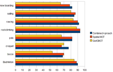
Our classification methods achieves 81.54 ± 1.62% and, so, for this dataset, the difference between the results for the proposed approach and for Spatial MCT is very small, less than 1%. Fig. 6 shows the comparison results among GistCMCT, spatial MCT and the proposed approach for one run experiment. We observe that the recognition rate, in the proposed approach, for the classes Sailing and Bocce are worst

Figure 5. Confusion matrix from one run for 15-class scene recognition experiment. Only rates higher or equal than 0.1 are shown in the figure.

(7)

than spatial MCT. For these cases the information brought from GistCMCT doesn't help at all.

4.5 Results on 67-class Indoor Scene

Recognition

In this dataset, we use 80 images in each category for training and 20 images for testing following [Qua09a]. All approaches presented here use the SVM classifier. Table 4 presents the results for this dataset.

Gist [Oli01a] 21

Global + local [Qua09a] 25

CENTRIST (3 levels) [Wu11a] 36.88 ± 1.10 Hibrid Representation [Niu10a] 40.19 GistCMCT [Gaz13a] 33.60 ± 1.30 Spatial MCT 38.58 ± 1.44

Ours (rule: max) 40.45 ± 1.41

Ours (rule: median) 41.83 ± 1.22

Ours (rule: product) 42.42 ± 1.32

Table 4. Experimental results for 67 class indoor scene categories dataset.

The experiments performed by [Qua09a] used local and global information to represent the scenes and the feature dimensions depends on the number of the Regions of Interest. In [Niu10a], a hybrid image representation by combining the global information with the local structure of the scene was proposed, generating a 34692 dimensions vector.

By using the proposed method we achieve 42.42 ± 1.32% employing the product rule and, as one can see, for this dataset, which contains only indoor scenes, the difference between the results for the

proposed approach and for Spatial MCT is close to 4%.

With respect to combining rule, the max rule achieved the worst results again.

5. CONCLUSION

In this paper, we proposed a new technique for scene classification by combing two classifiers based on different features, GistCMCT and spatial MCT, to improve classification performance. Combining classifiers allows the union of the complementary qualities of the two image descriptors without increasing the size of the feature vector. The experiments presented show the potential applicability of the technique. Nevertheless, when dealing with the recognition of events, the proposed approach did not bring a great vantage, as one can see in the results of events sports dataset, in which the results reached were very close to the spatial MCT approach results.

Besides the performance improvement, GistCMCT and spatial MCT are a holistic and low-dimensional representation of the structure of a scene and, also, don't require quantization of the data, as in the bag-of-features approach, which could be a computational expensive process.

In addition, the proposed approach is flexible and enables the use of different SVM kernels for each descriptor or, even, different kinds of classifiers, which can help to reach performance improvement through the choice of the most appropriate classifiers for each descriptor.

In future work, we plan to obtain contextual information from the different levels in the spatial layout and use other ways for combining classifiers by employing machine learning.

Figure 6. Classification rates by class for GistCMCT, spatial MCT and the combined approach from one run scene recognition experiment in the 8-class

(8)

[Erg10a] Ergul, E. and Arica, N. Scene classiﬁcation using spatial pyramid of latent topics. In Proceedings of the 2010 20th_{International Conference on Pattern}

Recognition, ICPR'10, pages: 3603–3606, 2010. [Fog07a] Foggia, P., Percannella, G., Sansone, C. and

Vento, M. Evaluating classiﬁcation reliability for combining classiﬁers. In Proceedings of the 14th International Conference on Image Analysis and Processing, ICIAP ’07, pages 711–716, 2007.

[Fro04a] Fröba, B. and Ernst, A. Face detection with the modiﬁed census transform. In Proceedings of the Sixth IEEE international conference on Automatic face and gesture recognition, pages 91–96, 2004.

[Gaz12a] Gazolli, K. and Salles, E. A contextual image descriptor for scene classification. In Online Proceedings on Trends in Innovative Computing, pages 66–71, 2012. [Online]. Available:

http://www.mirlabs.net/ict12/download/Paper13.pdf

[Gaz13a] Gazolli, K. and Salles E. Combining holistic descriptors for scene classification. In Proceedings of the International Conference on Computer Vision Theory and Applications (VISAPP 2013), pages 315– 320, 2013.

[Ho94a] Ho, K., Hull, J. J. and Srihari, S. N. Decision combination in multiple classiﬁer systems. IEEE Trans. Pattern Anal. Mach. Intell., pages 66–75, 1994. [Kit98a] Kittler,J., Hatef, M., Duin, R. P. W. and. Matas,

J. On combining classiﬁers. IEEE Trans. Pattern Anal. Mach. Intell., pages 226–239, 1998.

[Lab06a] Lazebnik, S., Schmid, C. and Ponce, J. Beyond bags of features: Spatial pyramid matching for recognizing natural scene categories. In Proceedings of the 2006 IEEE Computer Society Conference on Computer Vision and Pattern Recognition, CVPR ’06, pages 2169–2178, 2006.

[Li07a] Li, L.-J. and Fei-Fei. L. What, where and who? Classifying events by scene and object recognition. In IEEE 11th International Conference on Computer Vision, pages1–8, 2007.

[Li11a] Li, T., Mei, T., Kweon, I.-S. and Hua, X.-S. Contextual bag-of-words for visual categorization. Circuits and Systems for Video Technology, IEEE Transactions on, pages 381 –392, 2011 .

[Li11b] Li, Z. and Dewen, H . Scene classiﬁcation combining low-level and semantic modeling strategies. In Digital Manufacturing and Automation (ICDMA),

25th International Conference of, pages 1 –7, 2010. [Oli05a] Oliva, A. . Gist of the scene. Nature, pages 251–

257, 2005.

[Oli01a] Oliva A. and Torralba, A.. Modeling the shape of the scene: A holistic representation of the spatial envelope. Int. J. Comput.Vision, pages: 145–175, 2001.

[Oli06a] Oliva, A. and Torralba, A.. Building the gist of a scene: The role of global image features in recognition. Progress in Brain Research, page 23–36, 2006.

[Qua09a] Quattoni, A. and Torralba, A. Recognizing indoor scenes. In Proceedings IEEE CS Conf. Computer Vision and Pattern Recognition, pages 413– 420, 2009.

[Vap98a] Vapnik, V. The support vectormethod of function estimation. Nonlinear Modeling advanced blackbox techniques Suykens JAK Vandewalle J Eds, pages 55–85, 1998.

[Wu09a] Wu, J. and Rehg, J.M. Beyond the euclidean distance : Creating effective visual codebooks using the histogram intersection kernel. In Computer Vision, 2009 IEEE 12th International Conference on, pages 630–637, 2009.

[Wu11a] Wu, J. and Rehg, J. M. Centrist: A visual descriptor for scene categorization. IEEE Trans. Pattern Anal. Mach. Intell., pages 1489–1501, 2011. [Wu04a] Wu, T.-F., Lin, C.-J. and Weng. R. C.

Probability Estimates for Multi-class Classiﬁcation by Pairwise Coupling. Journal of Machine Learning Research 5, pages 975-1005, 2004.

[Zab94a] Zabih, R. and Woodﬁll, J. Non-parametric local transforms for computing visual correspondence. In Proceedings of the third European conference on Computer Vision - Volume 2, ECCV ’94, pages 151– 158, 1994.