Metaheuristics
Th´
e Van Luong, Nouredine Melab, El-Ghazali Talbi
To cite this version:
Th´
e Van Luong, Nouredine Melab, El-Ghazali Talbi. GPU Computing for Parallel Local Search
Metaheuristics. IEEE Transactions on Computers, Institute of Electrical and Electronics
En-gineers, 2013, 62 (1), pp.173-185.
<
inria-00638805
>
HAL Id: inria-00638805
https://hal.inria.fr/inria-00638805
Submitted on 7 Nov 2011
HAL
is a multi-disciplinary open access
archive for the deposit and dissemination of
sci-entific research documents, whether they are
pub-lished or not.
The documents may come from
teaching and research institutions in France or
abroad, or from public or private research centers.
L’archive ouverte pluridisciplinaire
HAL
, est
destin´
ee au d´
epˆ
ot et `
a la diffusion de documents
scientifiques de niveau recherche, publi´
es ou non,
´
emanant des ´
etablissements d’enseignement et de
recherche fran¸cais ou ´
etrangers, des laboratoires
publics ou priv´
es.
GPU Computing for Parallel Local Search
Metaheuristic Algorithms
Th ´e Van Luong, Nouredine Melab, El-Ghazali Talbi
Abstract—Local search metaheuristics (LSMs) are efficient methods for solving complex problems in science and industry. They allow
significantly to reduce the size of the search space to be explored and the search time. Nevertheless, the resolution time remains prohibitive when dealing with large problem instances. Therefore, the use of GPU-based massively parallel computing is a major complementary way to speed up the search. However, GPU computing for LSMs is rarely investigated in the literature. In this paper, we introduce a new guideline for the design and implementation of effective LSMs on GPU. Very efficient approaches are proposed for CPU-GPU data transfer optimization, thread control, mapping of neighboring solutions to GPU threads and memory management. These approaches have been experimented using four well-known combinatorial and continuous optimization problems and four GPU configurations. Compared to a CPU-based execution, accelerations up to×80are reported for the large combinatorial problems and up to×240for a continuous problem. Finally, extensive experiments demonstrate the strong potential of GPU-based LSMs compared
to cluster or grid-based parallel architectures.
Index Terms—Parallel Metaheuristics, Local Search Metaheuristics, GPU Computing, Performance Evaluation.
✦
1
I
NTRODUCTIONR
EAL-WORLD optimization problems are often com-plex and NP-hard. Their modeling is continu-ously evolving in terms of constraints and objectives, and their resolution is CPU time-consuming. Although near-optimal algorithms such as metaheuristics (generic heuristics) make it possible to reduce the temporal com-plexity of their resolution, they fail to tackle large prob-lems satisfactorily. GPU computing has recently been re-vealed effective to deal with time-intensive problems [1]. Our challenge is to rethink the design of metaheuristics on GPU for solving large-scale complex problems with a view to high effectiveness and efficiency. Metaheuristics are based on the iterative improvement of either single solution (e.g. Simulated Annealing or Tabu Search) or a population of solutions (e.g. evolutionary algorithms) of a given optimization problem. In this paper, we focus on the first category i.e. local search metaheuristics. This class of algorithms handles a single solution which is iteratively improved by exploring its neighborhood in the solution space. The neighborhood structure depends on the solution encoding which could mainly be a binary encoding, a vector of discrete values, a permutation or a vector of real values.For years, the use of GPU accelerators was devoted to graphics applications. Recently, their use has been extended to other application domains [2] (e.g. compu-tational science) thanks to the publication of the CUDA [3] (Compute Unified Device Architecture) development toolkit that allows GPU programming in C-like lan-guage. In some areas such as numerical computing [4],
• T.V. Luong, N. Melab and E-G. Talbi are from both INRIA Lille Nord Europe and CNRS/LIFL Labs, Universit´e de Lille1, France (e-mail: [email protected]; [email protected]; [email protected])
we are now witnessing the proliferation of software libraries such as CUBLAS for GPU. However, in other areas such as combinatorial optimization, the spread of GPU does not occur at the same pace. Indeed, there only exists few research works related to evolutionary algorithms on GPU [5]–[7].
Nevertheless, parallel combinatorial optimization on GPU is not straightforward and requires a huge effort at design as well as at implementation level. Indeed, several scientific challenges mainly related to the hier-archical memory management have to be achieved. The major issues are efficient distribution of data processing between CPU and GPU, thread synchronization, opti-mization of data transfer between the different memo-ries, the capacity constraints of these memomemo-ries, etc. The main purpose of this paper is to deal with such issues for the re-design of parallel LSM models in order to solve large scale optimization problems on GPU architectures. We propose a new generic guideline for building efficient parallel LSMs on GPU.
Different contributions and salient issues are dealt with: (1) defining an effective cooperation between CPU and GPU, which requires to optimize the data trans-fer between the two components; (2) GPU computing is based on hyper-threading (massively parallel multi-threading), and the order in which the threads are exe-cuted is not known. Therefore, on the one hand, an effi-cient thread control must be applied to meet the memory constraints. On the other hand, an efficient mapping has to be defined between each neighboring candidate solution and a thread designated by a unique identifier assigned by the GPU runtime; (3) the neighborhood has to be placed efficiently on the different memories taking into account their sizes and access latencies.
prob-lems with different encodings have been considered on GPU: the quadratic assignment problem (QAP) [8], the permuted perceptron problem (PPP) [9], the trav-eling salesman problem (TSP) [10], and the continuous Weierstrass function [11]. QAP and TSP are permutation problems; PPP is based on the binary encoding, and the Weierstrass function is represented by a vector of real values. The proposed work has been experimented on the four problems using four GPU configurations. These latter have different performance capabilities in terms of threads that can be created simultaneously and memory caching.
The remainder of the paper is organized as follows: Section 2 highlights the principles of parallel LSMs. Sec-tion 3 describes generic concepts for designing parallel LSMs on GPU. In Section 4, parallelism control through efficient mappings between state-of-the-art LSM struc-tures and GPU threads model is performed. A thorough examination of the GPU memory management adapted to LSMs is conducted in Section 5. Section 6 reports the performance results obtained for the implemented problems. Finally, a discussion and some conclusions of this work are drawn in Section 7.
2
P
ARALLELL
OCALS
EARCHM
ETAHEURIS-TICS
2.1 Principles of Local Search Metaheuristics LSMs are search techniques that have been successfully applied for solving many real and complex problems. They could be viewed as “walks through neighbor-hoods” meaning search trajectories through the solutions domains of the problems at hand. The walks are per-formed by iterative procedures that allow to move from one solution to another (see Algorithm 1).
A LSM starts with a randomly generated solution. At each iteration of the algorithm, the current solution is replaced by another one selected from the set of its neighboring candidates, and so on. An evaluation func-tion associates a fitness value to each solufunc-tion indicating its suitability to the problem. Many strategies related to the considered LSM can be applied in the selection of a move: best improvement, first improvement, random selection, etc. A survey of the history and a state-of-the-art of LSMs can be found in [12].
Algorithm 1Local search pseudo-code
1: Generate(s0); 2: Specific LSM pre-treatment 3: t:=0; 4: repeat 5: m(t):= SelectMove(s(t)); 6: s(t+ 1) := ApplyMove(m(t), s(t)); 7: Specific LSM post-treatment 8: t:=t+ 1;
9: untilTermination criterion(s(t))
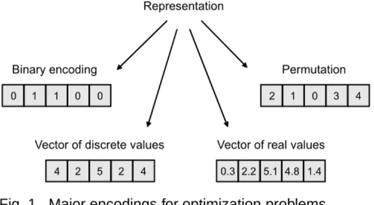
Fig. 1. Major encodings for optimization problems.
2.2 Solution Representation
Designing any iterative metaheuristic requires an encod-ing of a solution. The representation plays a leadencod-ing role in the efficiency and effectiveness of any LSM. It must be suitable and relevant to the optimization problem at hand. Moreover, the quality of a representation has a considerable influence on the efficiency of the search operators applied on this representation (neighborhood). Four main encodings in the literature can be highlighted: binary encoding (e.g. Knapsack, SAT), vector of discrete values (e.g. location problem, assignment problem), per-mutation (e.g. TSP, scheduling problems) and vector of real values (e.g. continuous functions). Fig. 1 illustrates an example of each representation.
2.3 Parallel Models of Local Search Metaheuristics Various algorithmic issues are being studied to design efficient LSMs. These issues commonly consist in defin-ing new move operators, parallel models, and so on. Parallelism naturally arises when dealing with a neigh-borhood, since each of the solutions belonging to it is an independent unit. Performance of LSMs is thus remarkably improved when running in parallel.
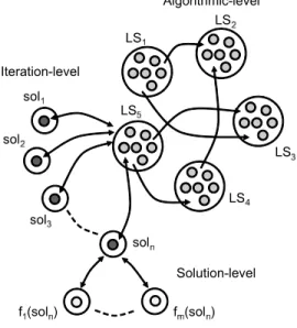
Three major parallel models for LSMs can be distin-guished: solution-level, iteration-level and algorithmic-level (see Fig. 2).
• Solution-level Parallel Model. The focus is on the parallel evaluation of a single solution. This model is particularly appealing when the evaluative func-tion can itself be parallelized as it is CPU time-consuming and/or IO intensive. In that case, the function can be viewed as an aggregation of partial functions.
• Iteration-level Parallel Model. This model is a low-level Master-Worker model that does not alter the behavior of the heuristic. Evaluation of the neigh-borhood is made in parallel. At the beginning of each iteration, the master duplicates the current solution between parallel nodes. Each of them man-ages a number of candidates, and the results are returned back to the master.
• Algorithmic-level Parallel Model. Several LSMs are simultaneously launched for computing robust solu-tions. They may be heterogeneous or homogeneous,
Fig. 2. Parallel models of local search metaheuristics.
independent or cooperative, started from the same or different solution(s) and configured with the same or different parameters.
2.4 GPU Computing for Local Search Metaheuristics During these two last decades, different parallel ap-proaches and implementations have been proposed for LSM algorithms using Massively Parallel Processors [13], Clusters of Workstations (COWs) [14]–[16] and Shared Memory or SMP machines [17], [18]. These contributions have been later revisited for large-scale computational grids [19].
These architectures often exploit the coarse-grained asynchronous parallelism based on work-stealing. This is particularly the case for computational grids. To over-come the problem of network latency, the grain size is often increased, limiting the degree of parallelism.
Recently, GPU accelerators have emerged as a pow-erful support for massively parallel computing. Indeed, these architectures offer a substantial computational horsepower and a remarkably high memory bandwidth compared to CPU-based architectures. Since more tran-sistors are dedicated to data processing rather than data caching and flow control, GPU is reserved for compute-intensive and highly parallel computations. Reviews of GPU architectures can be found in [1], [20].
The parallel evaluation of the neighborhood (iteration-level) is a Master-Worker and a problem-independent, regular data-parallel application. Therefore, GPU com-puting is highly efficient in executing such synchronized parallel algorithms that involve regular computations and data transfers.
In general, for distributed architectures, the global performance in metaheuristics is limited by high com-munication latencies whilst it is just bounded by mem-ory access latencies in GPU architectures. Indeed, when evaluating the neighborhood in parallel, the main
draw-back in distributed architectures is the communication efficiency. GPUs are not that versatile.
However, since the execution model of GPUs is purely SIMD, it may not be well-adapted for few irregular problems in which the execution time cannot be pre-dicted at compile time and varies during the search. For instance, this happens when the evaluation cost of the objective function depends on the solution. When dealing with such problems in which the computations or the data transfers become irregular or asynchronous, parallel and distributed architectures such as COWs or computational grids may be more appropriated.
3
D
ESIGN OFP
ARALLELL
OCALS
EARCHM
ETAHEURISTICS ONGPU
In this section, the focus is on the re-design of the iteration-level parallel model presented in Section 2.3. 3.1 Generation of the Neighborhood
The GPU has its own memory and processing ele-ments that are separate from the host computer. Thereby, CPU/GPU communication might be a serious bottleneck in the performance of GPU applications. One of the crucial issues is to optimize the data transfer between the CPU and the GPU. Regarding LSMs, these copies represent the solutions to be evaluated. In other words, one has to say where the neighborhood must be gener-ated. For doing that, there are basically two approaches:
• Generation of the neighborhood on CPU and its evalua-tion on GPU. At each iteration of the search process, the neighborhood is generated on the CPU side. Its associated structure storing the solutions is copied on GPU. Thereby, the data transfers are essentially the set of neighboring solutions copied from the CPU to the GPU. This approach is straightforward since a thread is automatically associated with its physical neighbor representation.
• Generation of the neighborhood and its evaluation on GPU. In the second approach, the neighborhood is generated on GPU. It implies that no explicit structure needs to be allocated. This is achieved by considering a neighbor as a slight variation of the candidate solution which generates the neigh-borhood. Thereby, only the representation of this candidate solution must be copied from the CPU to the GPU. The benefit of such an approach is to reduce drastically the data transfers since the whole neighborhood does not have to be copied. However, finding a mapping between a thread and a neighbor might be challenging. Such an issue will be discussed in Section 4.2.
The first approach is easier, but it will end in a lot of data transfers for large neighborhoods, leading to a great loss of performance. That is the reason why, in the rest of the paper, we will consider the second approach. An experimental comparison of the two approaches is broached in Section 6.
3.2 The Proposed GPU-based Algorithm
Adapting traditional LSMs to GPU is not an easy task. We propose a methodology to adapt LSMs on GPU in a generic way (see Algorithm 2).
Algorithm 2Local Search Template on GPU
1: Choose an initial solution
2: Evaluate the solution
3: Specific LSM initializations
4: Allocate problem inputs on GPU memory
5: Allocate a solution on GPU memory
6: Allocate a fitnesses structure on GPU memory
7: Allocate additional structures on GPU memory
8: Copy problem inputs on GPU memory
9: Copy the initial solution on GPU memory
10: Copy additional structures on GPU memory
11: repeat
12: foreach neighbor in paralleldo
13: Incremental evaluation of the candidate solution 14: Insert the resulting fitness into the fitnesses
structure
15: end for
16: Copy the fitnesses structure on CPU memory
17: Specific LSM selection strategy on the fitnesses structure
18: Specific LSM post-treatment
19: Copy the chosen solution on GPU memory
20: Copy additional structures on GPU memory
21: untila stopping criterion satisfied
First of all, at initialization stage, memory allocations on GPU are made: data inputs and candidate solution of the given problem (lines 4 and 5). A structure has to be allocated for storing the results of the evaluation of each neighbor (fitnesses structure) (line 6). Addi-tional structures, which are problem-dependent, might be allocated to facilitate the computation of neighbors evaluations (line 7). Second, problem data inputs, initial candidate solution and additional structures associated with this solution have to be copied onto the GPU (lines 8 to 10). Third, comes the parallel iteration-level on GPU, in which each neighboring solution is generated (parallelism control), evaluated (memory management) and copied into the fitnesses structure (from lines 12 to 15). Fourth, the order in which candidate neighbors are evaluated is undefined, then the fitnesses structure has to be copied to the host CPU (line 16). Then a solution selection strategy is applied to this structure (line 17): the exploration of the neighborhood fitnesses structure is carried out by the CPU in a sequential way. Finally, after a new candidate has been selected, this latter and its additional structures are copied to the GPU (lines 19 and 20). The process is repeated until a stopping criterion is satisfied.
This methodology is well-adapted to any deterministic LSMs. Its applicability does not stand on any assump-tion.
3.3 Additional Data Transfer Optimization
In some LSMs such as Hill Climbing or Variable Neigh-borhood Descent, the selection operates on the minimal fitness for finding the best solution. Therefore, only one value of the fitnesses structure has to be copied from the GPU to the CPU. However, finding the proper minimal fitness in parallel on GPU is not direct. To deal with this issue, adaptation of parallel reduction techniques [21] for each thread block must be considered. Thus, by using local synchronizations between threads in a given block via the shared memory, one can find the minimum of a given structure. The complexity of such an algorithm is inO(log2(n)), wherenis the size of each threads block.
The benefits of such a technique for LSMs will be pointed out in Section 6.
4
P
ARALLELISMC
ONTROL OFL
OCALS
EARCHM
ETAHEURISTICS ONGPU
In this section, the focus is on the neighborhood gener-ation to control the threads parallelism.
4.1 Thread Control
From an hardware point of view, GPU multiproces-sor is based on thread-level parallelism to maximize the exploitation of its functional units. Each processor device on GPU supports the single program multiple data (SPMD) model, i.e. multiple autonomous processors simultaneously execute the same program on different data. For achieving this, the kernel is a function callable from the CPU host and executed on the specified GPU device. It defines the computation to be performed by a large number of threads, organized in thread blocks. The multiprocessor executes threads in groups of32threads calledwarps. Blocks of threads are partitioned into warps that are organized by a scheduler at runtime.
Hence, one of the key points to achieve high per-formance is to keep the GPU multiprocessors as active as possible. Latency hiding depends on the number of active warps per multiprocessor, which is implicitly determined by the execution parameters along with reg-ister constraints. That is the reason why, it is necessary to use threads and blocks in a way that maximizes hardware utilization. This is achieved with two param-eters: the number of threads per block and the total number of threads. In general, threads per block should be a multiple of the warp size (i.e.32 threads) to avoid wasting computation on under-populated warps.
Regarding the execution of a LSM on GPU, it consists in launching a kernel with a large number of threads. In this case, one thread is associated with one neighbor. However, for an extremely large neighborhood set, some experiments might not be conducted. The main issue is then to control the number of threads to meet the memory constraints like the limited number of registers to be allocated to each thread. As a result, on the one hand, having an efficient thread control will prevent
GPU programs from crashing. On the other hand, it will allow to find an optimal number of threads required at launch time to obtain the best multiprocessor occupancy. Different works [22], [23] have been investigated for parameters auto-tuning. The heuristics are a priori ap-proaches which consist in enumerating all the different values of the two parameters (threads per block and number of threads). Such approaches are too much time-consuming and are not well-adapted to LSMs.
We propose in Algorithm 3 a dynamic heuristic for parameters auto-tuning. The main idea of this approach is to send threads by “waves” to the GPU kernel to perform the parameters tuning during the first LSM iterations. Thereby, the time measurement for each se-lected configuration, according to a certain number of trials (lines 5 to 14), will deliver the best configuration parameters. Regarding the number of threads per block, as quoted above, it is set as a multiple of the warp size (see line 19). The starting total number of threads is set as the nearest power of two of the solution size, as well. For decreasing the total number of configurations, the algorithm terminates when the logarithm of the neighborhood size is reached. In some cases, the kernel execution will fail since too many threads are requested. Therefore, a fault-tolerance mechanism is provided to detect such a situation (from lines 8 to 12). In this case, the heuristic terminates and returns the best configura-tion parameters previously found.
Algorithm 3Dynamic parameters tuning heuristic
Require: nb trials;
1: nb threads := nearest power of 2 (solution size);
2: whilenb threads<=neighborhood sizedo
3: nb threads block := 32;
4: whilenb threads block<=512do
5: repeat
6: LSM iteration pre-treatment on host side
7: Generation and evaluation kernel on GPU
8: ifGPU kernel failurethen
9: Restore (best nb threads);
10: Restore (best nb threads block);
11: Exit procedure
12: end if
13: LSM iteration post-treatment on host side
14: untilTime measurements of nb trials
15: ifBest time improvementthen
16: best nb threads := nb threads;
17: best nb threads block := nb threads block;
18: end if
19: nb threads block := nb threads + 32; 20: end while
21: nb threads := nb threads * 2;
22: end while
23: Exit procedure
Ensure: best nb threads and best nb threads block;
The only parameter to determine is the number of
Fig. 3. A neighborhood for binary representation.
trials per configuration. The more this value is, the more will be accurate the overall tuning at the expense of an extra computational time. The benefits of the thread control will be presented in Section 6.
4.2 Efficient Mapping of Neighborhood Structures on GPU
The neighborhood structures play a crucial role in the performance of LSMs and are problem-dependent. As quoted above, a kernel is launched with a large number of threads which are provided with a unique id. As a consequence, the main difficulty is to find an efficient mapping between a GPU thread and LSM neighboring solutions. The answer is dependent of the solution rep-resentation. In the following, we provide a methodology to deal with the main structures of the literature. 4.3 Binary Encoding
In a binary representation, a solution is coded as a vec-tor of bits. The neighborhood representation for binary problems is usually based on Hamming distance (see Fig. 3). A neighbor of a given solution is obtained by flipping one bit of the solution.
Mapping between LSM neighborhood encoding and GPU threads is fairly trivial. Indeed, on the one hand, for a binary vector of sizen, the size of the neighborhood is exactlyn. On the other hand, threads are provided with a uniqueid. That way, a thread is directly associated with at least one neighbor.
4.4 Discrete Vector Representation
Discrete vector representation is an extension of binary encoding using a given alphabet Σ. In this representa-tion, each variable acquires its value from the alphabet
Σ. Assuming that the cardinality of the alphabet Σ is
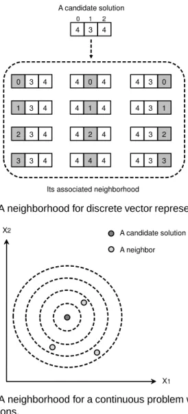
k, the size of the neighborhood is (k −1) ×n for a discrete vector of lengthn. Fig. 4 illustrates an example of discrete representation withn= 3and k= 5.
Let id be the identity of the thread corresponding to a given candidate solution of the neighborhood. Com-pared to the initial solution which allowed to generate
Fig. 4. A neighborhood for discrete vector representation.
Fig. 5. A neighborhood for a continuous problem with two dimensions.
the neighborhood, id/(k −1) represents the position which differs from the initial solution and id%(k−1)
is the available value from the ordered alphabet Σ. Therefore, such a mapping is possible.
4.5 Vector of Real Values
For continuous optimization, a solution is coded as a vector of real values. A usual neighborhood for such a representation consists in discretizing the solution space. The neighborhood is defined in [24] by using the concept of “ball”. A ball B(s, r) is centered on s with radiusr; it contains all points s0
such that ||s0
−s|| ≤ r. A set of balls centered on the current solution sis considered with radiush0,h1, . . . ,hm.
Thus, the space is partitioned into concentric “crowns” Ci(s, hi−1, hi) such that Ci(s, hi−1, hi) =
s0
|hi−1≤ ||s0−s|| ≤hi. Themneighbors ofsare chosen
by random selection of one point inside each crown Ci
forivarying from1tom(see Fig. 5). This can be easily done by geometrical construction. The mapping consists in associating one thread with at least one neighbor corresponding to one point inside each crown.
Fig. 6. A neighborhood for permutation representation.
4.6 Permutation Representation
4.6.1 2-exchange Neighborhood
Building a neighborhood by pair-wise exchange opera-tions is a typical way for permutation problems. For a permutation of lengthn, the size of the neighborhood is
n×(n−1)
2 . Fig. 6 illustrates a permutation representation
and its associated neighborhood.
Unlike the previous representations, in the case of a permutation encoding, the mapping between a neighbor and a GPU thread is not straightforward. Indeed, on the one hand, a neighbor is composed of two indexes (a swap in a permutation). On the other hand, threads are identified by a unique id. Consequently, one mapping has to be considered to transform one index into two ones. In a similar way, another one is required to convert two indexes into one.
Proposition 1: Two-to-one index transformation
Given i and j the indexes of two elements to be exchanged in the permutation representation, the corresponding index f(i, j) in the neighborhood representation is equal toi×(n−1) + (j−1)−i×(i+1)
2 ,
wherenis the permutation size.
Proposition 2: One-to-two index transformation
Given f(i, j) the index of the element in the neighborhood representation, the corresponding indexi
is equal ton−2− b √ 8×(m−f(i,j)−1)+1−1 2 candj is equal to f(i, j)−i×(n−1) +i×(i+1) 2 + 1 in the permutation
representation, where n is the permutation size andm
the neighborhood size.
The proofs of two-to-one and one-to-two index transfor-mations can be found in Appendix A.1 and Appendix A.2. Another well-known neighborhood for permutation problems is a neighborhood built by exchanging three values. Its full details and mappings are discussed in Appendix A.3.
5
M
EMORYM
ANAGEMENT OFL
OCALS
EARCHM
ETAHEURISTICS ONGPU
Task repartition between the CPU and the GPU and efficient parallelism control in LSMs have been pre-viously proposed. In this section, the focus is on the memory management. Understanding the GPU memory organization and its related issues is useful to provide an efficient implementation of parallel LSMs.
5.1 Memory Coalescing Issues
From an hardware point of view, at any clock cycle, each processor of the multiprocessor selects a half-warp (16 threads) that is ready to execute the same instruction on different data. Global memory is conceptually organized into a sequence of 128-byte segments. The number of memory transactions performed for a half-warp will be the number of segments having the same addresses as used by that half-warp.
For more efficiency, global memory accesses must be coalesced, which means that a memory request per-formed by consecutive threads in a half-warp is strictly associated with one segment. If per-thread memory accesses for a single half-warp establish a contiguous range of addresses, accesses will be coalesced into a sin-gle memory transaction. Otherwise, accessing scattered locations results in memory divergence and requires the processor to produce one memory transaction per thread.
Regarding LSMs, global memory accesses in the eval-uation function have a data-dependent unstructured pat-tern (especially for permutation representation). There-fore, non-coalesced memory accesses involve many memory transactions, which lead to a significant per-formance decrease for LSMs. Appendix B.1 exhibits a pattern of coalescing transformation for dealing with intermediate structures used in combinatorial problems. Notice that, in the Fermi based GPUs, global memory is easier to access. This is due to the relaxation of the coalescing rules and the presence of L1 cache memory. It means that applications developed on GPU get a better global memory performance on this card.
5.2 Texture Memory
The use of texture memory is a solution for reduc-ing memory transactions due to non-coalesced accesses. Texture memory provides a surprising aggregation of capabilities including the ability to cache global memory. Indeed, each texture unit has some internal memory that buffers data from global memory. Therefore, texture memory can be seen as a relaxed mechanism for the threads to access the global memory. Indeed, the coa-lescing requirements do not apply to texture memory accesses. Thereby, the use of texture memory is well-adapted for LSMs for the following reasons:
• Data accesses are repeated in the computation of LSM evaluation functions.
TABLE 1
Kernel memory management. Summary of the different memories used in the evaluation function.
Type of memory LSM structure
Texture memory problem inputs, solution representation Global memory fitnesses structure, large structures
Registers additional variables Local memory small structures Shared memory partial fitnesses structure
• This memory is adapted to LSMs since the problem data and the solution representation are read-only values.
• Since optimization problem inputs are mostly 2D matrices or 1D solution vectors, cached texture data is laid out so as to give the best performance for 1D/2D access patterns.
The use of textures in place of global memory accesses is a totally mechanical transformation. Details of texture coordinate clamping and filtering is given in [3], [21]. 5.3 Memory Management
Table 1 summarizes the memory management in accor-dance with the different LSM structures. The inputs of the problem (e.g. matrix in TSP) and the solution which generates the neighborhood are associated with the tex-ture memory. The fitnesses structex-ture which stores the obtained results for each neighbor is declared as global memory (only one writing operation). Declared variables for the computation of each neighbor are automatically associated with registers by the compiler. Additional complex structures, which are private to a neighbor, will reside in local memory. In the case where these structures are too large to fit into local memory, they are stored in global memory using the coalescing transformation mentioned above. Finally, the shared memory may be used to perform additional reduction operations on the fitness structure to collect the minimal/maximal fitness. A discussion, which explains why its use is not adapted for LSMs, is proposed in Appendix B.2.
6
E
XPERIMENTATIONIn order to validate the approaches presented in this paper, the four problems presented in the introduction have been implemented. As the iteration-level parallel model does not change the semantics of the sequential algorithm, the effectiveness in terms of quality of solu-tions is not addressed here. Only execution times and acceleration factors are reported in comparison with a single-core CPU.
For the four problems, a Tabu Search has been im-plemented on GPU. This algorithm enhances the perfor-mance of the search by using memory structures. Indeed, the main memory structure called the tabu list represents the history of the search trajectory. In this way, using this list allows to avoid cycles during the search process.
Experiments have been carried out on top of four different configurations. The GPU cards have a different number of cores (respectively 32, 128, 240 and 448), which determines the number of active threads being executed. The three first cards are relatively modest and old, whereas the last one is a modern Fermi card. The number of global iterations of the Tabu Search is set to 10000 which corresponds to a realistic scenario in accordance with the algorithm convergence. For the different problems, a single-core CPU implementation, a CPU-GPU, and a CPU-GPU version using texture mem-ory (GP Utex) are considered for each configuration. The number of threads per block has been arbitrary chosen to 256(multiple of32), and the total number of threads created at run time is equal to the neighborhood size. The additional thread control to adjust parameters will be specifically applied to some problems. The average time has been measured in seconds for 30 runs. For the sake of clarity, the CPU time is not represented in most tables since it can be deduced. Statistical analysis of all the produced results can be found in Appendix D. 6.1 Application to the Quadratic Assignment Prob-lem
The QAP arises in many applications such as facility location or data analysis. Let A = (aij) and B = (bij)
be n×n matrices of positive integers. Finding a solu-tion of the QAP is equivalent to finding a permutasolu-tion
π= (1,2, . . . , n)that minimizes the objective function:
z(π) = n X i=1 n X j=1 aijbπ(i)π(j)
The problem has been implemented using a permu-tation represenpermu-tation. The neighbor evaluation function has a time complexity of O(n), and the number of created threads is equal to n×(n−1)
2 . The considered
instances are the Taillard instances proposed in [8]. They are uniformly generated and are well-known for their difficulty. Results are shown in Table 2 for the four configurations. Non-coalescing memory drastically re-duces the performance of GPU implementation on both G80 cards. This is due to high-misaligned accesses to global memories (flows and distances in QAP). Bind-ing texture on global memory allows to overcome the problem. Indeed, from the instance tai30a, using texture memory starts providing positive acceleration factors for both configurations (respectively ×1.8, ×1.9, ×2.0
and ×2.8). GPU keeps accelerating the search as long as the size grows. Regarding the GTX 280, this card provides twice as many multiprocessors and registers. As a consequence, hardware capability and coalescing rules relaxation lead to a significant speed-up (from
×10.9 to ×16.5 for the biggest instance tai100a). The same goes on for the Tesla M2050 where the acceleration factor varies from ×15.7 to ×18.6. However, since this last card provides on-chip memory for L1 cache memory, the benefits of texture memory are less pronounced.
6.2 Application to the Permuted Perceptron Problem
In [9], Pointcheval introduced a cryptographic identifi-cation scheme based on the perceptron problem, which seems to be suited for resource-constrained devices such as smart cards. An -vector is a vector with all entries being either +1 or -1. Similarly, an-matrix is a matrix in which all entries are either +1 or -1. The PPP is defined as follows:
Definition 1: Given an -matrix A of size m × n
and a multi-set S of non-negative integers of size m, find an -vector V of size n such that
{{(AV)j/j={1, . . . , m}}}=S.
PPP has been implemented using a binary encoding. Part of the full evaluation of a solution can be seen as a matrix-vector product. Therefore, the evaluation of a neighbor can be performed in linear time. Experimental results for a Hamming neighborhood of distance one are depicted in Table 3 (m-ninstances). From m= 401and
n= 417, the GPU version using texture memory starts to be faster than the CPU one for both configurations (from
×1.7 to ×3.6). Since accesses to global memory in the evaluation function are minimized, the GPU implemen-tation is not much affected by non-coalescing memory operations. Indeed, from m = 601 and n = 617, the GPU version without any texture memory use starts to provide better results (from×1.1 to ×4). The speed-up grows with the problem size augmentation (up to ×12
for m = 1301, n = 1317). The acceleration factor for this implementation is significant but not spectacular. Indeed, since the neighborhood is relatively small (n
threads), the number of threads per block is not enough to cover fully the memory access latency.
To validate this point, a Hamming neighborhood of distance two has been implemented. The evaluation kernel is executed by n×(n2−1) threads. The obtained results from experiments are reported in Table 4. For the first instance (m = 73, n = 73), acceleration factors of the texture version are already significant (from×3.6 to
×12.3). As long as the instance size increases, the ac-celeration factor grows accordingly (from×3.6to×8for the first configuration). Since a large number of cores are available on both 8800 and GTX 280, efficient speed-ups can be obtained (from×10.1 to ×44.1). The application also scales well when performing on the Tesla Fermi card (speed-ups varying from×11.7 to×73.3).
Details about the benefits of coalescing transformation for this problem are discussed in Appendix C.3.
A conclusion from these experiments indicates that parallelization on top of GPU provides a highly efficient way for handling large neighborhoods. The same goes on with a neighborhood based on a Hamming distance three (see Appendix C.2).
TABLE 2
Measures in terms of efficiency for the QAP using a pair-wise-exchange neighborhood.
Instance
Core 2 Duo T5800 Core 2 Quad Q6600 Xeon E5450 Xeon E5620
GeForce 8600M GT GeForce 8800 GTX GeForce GTX 280 Tesla M2050
32 GPU cores 128 GPU cores 240 GPU cores 448 GPU cores
GPU GPUTex GPU GPUTex GPU GPUTex GPU GPUTex
tai30a 4.2×0.5 1.3×1.8 2.3×0.8 1.0×1.9 1.1×1.4 0.8×2.0 0.5×2.2 0.4×2.8 tai35a 6.5×0.5 1.6×2.1 2.9×0.9 1.2×2.3 1.2×1.9 0.9×2.6 0.6×2.4 0.5×3.8 tai40a 9.7×0.5 1.8×2.6 3.7×1.1 1.5×2.9 1.3×2.7 1.1×3.3 0.7×3.2 0.5×4.4 tai50a 16×0.6 3.0×3.2 5.7×1.4 1.8×4.6 1.7×4.1 1.3×5.3 0.8×5.4 0.6×7.2 tai60a 28×0.6 4.9×3.4 8.4×1.6 2.0×7.1 2.0×5.6 1.6×7.3 1.1×8.4 0.9×10.2 tai80a 63×0.7 10×4.2 19×1.9 4.5×8.1 3.2×9.1 2.8×10.8 1.9×12.4 1.7×13.5 tai100a 139×0.8 19×5.6 33×2.3 8.7×8.8 5.5×10.9 3.7×16.5 3.1×15.7 2.6×18.6 TABLE 3
Measures in terms of efficiency for the PPP using a neighborhood based on a Hamming distance of one.
Instance
Core 2 Duo T5800 Core 2 Quad Q6600 Xeon E5450 Xeon E5620
GeForce 8600M GT GeForce 8800 GTX GeForce GTX 280 Tesla M2050
32 GPU cores 128 GPU cores 240 GPU cores 448 GPU cores
GPU GP UT ex GPU GP UT ex GPU GP UT ex GPU GP UT ex 73-73 6.1×0.2 5.0×0.3 3.3×0.3 3.0×0.4 3.5×0.3 2.8×0.5 1.8×0.6 1.7×0.7 81-81 6.7×0.3 5.3×0.3 3.9×0.4 3.5×0.4 3.8×0.3 3.1×0.5 2.1×0.6 2.0×0.7 101-117 8.9×0.4 6.6×0.5 4.8×0.5 4.3×0.6 4.9×0.4 3.9×0.6 2.2×1.1 2.1×1.2 201-217 19×0.6 12×0.9 10×0.8 8.1×1.1 8.8×0.9 7.7×1.1 4.9×2.1 4.6×2.2 401-417 53×0.8 24×1.7 28×1.2 18×1.8 16×1.9 13×2.2 8.9×3.4 8.4×3.6 601-617 169×1.1 98×1.9 96×1.6 68×2.2 47×2.2 43×2.4 26×4.0 25×4.1 801-817 244×1.4 120×3.1 120×2.4 84×3.4 54×3.6 49×4.2 31×6.3 28×6.9 1001-1017 345×1.8 147×4.1 145×3.1 100×4.5 63×5.3 60×5.7 45×8.5 42×9.1 1301-1317 571×2.2 273×4.3 227×3.6 169×4.8 93×7.4 82×8.1 62×11.2 58×12.0 TABLE 4
Measures in terms of efficiency for the PPP using a neighborhood based on a Hamming distance of two.
Instance
Core 2 Duo T5800 Core 2 Quad Q6600 Xeon E5450 Xeon E5620
GeForce 8600M GT GeForce 8800 GTX GeForce GTX 280 Tesla M2050
32 GPU cores 128 GPU cores 240 GPU cores 448 GPU cores
GPU GPUTex GPU GPUTex GPU GPUTex GPU GPUTex
73-73 3.9×0.7 0.8×3.6 1.3×1.7 0.2×10.1 0.2×9.9 0.2×10.9 0.2×11.7 0.2×12.3 81-81 5.2×0.8 1.1×3.8 1.7×1.7 0.3×10.4 0.3×10.3 0.2×12.2 0.2×12.8 0.2×13.4 101-117 12×0.9 2.5×4.4 4.1×1.8 0.6×12.4 0.6×11.8 0.4×18.1 0.4×21.1 0.3×22.0 201-217 75×0.9 15×4.7 25×2.0 3.3×15.4 3.0×16.3 1.9×25.3 1.7×28.7 1.6×30.6 401-417 570×1.0 103×5.4 123×3.5 24×18.3 20×20.1 14×28.8 11×37.4 10×38.3 601-617 1881×1.7 512×6.3 351×7.1 89×28.3 67×30.5 51×40.1 37×55.2 35×58.4 801-817 4396×2.0 1245×6.9 817×8.5 212×32.8 154×35.3 128×42.3 86×63.2 81×67.1 1001-1017 8474×2.1 2421×7.2 1474×9.8 409×35.2 292×37.9 252×43.9 162×68.3 154×71.9 1301-1317 17910×2.2 4903×8.0 3041×10.9 911×36.2 651×38.5 568×44.1 362×69.2 342×73.3
6.3 Application to the Weierstrass Continuous Function
The Weierstrass functions belong to the class of con-tinuous optimization problems. These functions have been widely used for the simulation of fractal surfaces. According to [11], Weierstrass-Mandelbrot functions are defined as follows:
Wb,h(x) =
∞ X
i=1
b−ihsin(bix) with b >1and0< h <1
(1) The parameter h has an impact on the irregularity (“noisy” local perturbation of limited amplitude) and these functions possess many local optima. The problem has been implemented using a vector of real values. The domain definition has been set to −1 ≤ xk ≤ 1,
h has been fixed to 0.25, and the number of iterations to compute the approximation to 100 (instead of ∞). Such parameters are in accordance with the one dealt with in [11]. The complexity of the evaluation function is quadratic. The texture optimization is not applied since there are no data inputs in continuous optimization problem.
10000 neighbors are considered with a maximal ra-dius equals to 1
n where n is the problem dimension.
The results obtained for the different configurations are reported in Table 5 for single precision floating-point. In comparison with the previous experiments, the first thing that is highlighted concerns the impressive ob-tained speed-ups. They alternate from ×39.2 to ×243
according to the different configurations, and they grow with the instance size augmentation. This can be clarified
by the fact that there are no data inputs thus no addi-tional memory access latencies. Table 4 in Appendix C.4 confirms a similar observation of the performance results when increasing the neighborhood size.
Regarding the quality of solutions, a preliminary study has been investigated in Appendix C.4.1. It points out the accuracy difference of produced solutions, when using single or double precision floating-point.
6.4 Application to the Traveling Salesman Problem Given n cities and a distance matrix dn,n, where each element dij represents the distance between the cities i
andj, the TSP consists in finding a tour which minimizes the total distance. A tour visits each city exactly once.
The chosen representation is a permutation structure. A swap operator for the TSP has been implemented on GPU. The considered instances have been selected among the TSPLIB instances presented in [10]. Table 6 presents the results for the TSP implementation. On the one hand, even if a large number of threads are executed (n×(n−1)
2 neighbors), the values for the first configuration
are not significant (acceleration factor from×1.2to×1.5
for the texture version). Indeed, the neighbor evaluation function consists of replacing two to four edges of a solution. As a result, this computation can be given in constant time, which is not enough to hide the memory latency. Regarding the other configurations, using more cores overcomes the issue, and yields a better global performance. Indeed, for the GeForce 8800, with the use of texture memory, accelerations start from ×1.5 with the eil101 instance and grows up to ×4.4 for pr2392. In a similar manner, GTX 280 starts from×2.3and goes up to an acceleration factor of ×11for the fnl4461 instance. Nevertheless, for the three first configurations, for larger instances such as pr2392, fnl4461 or rl5915, the program has provoked an execution error because of the hardware register limitation.
6.5 Thread Control
Since the GPU may fail to execute large neighborhoods on large instances, the next experiment consists in high-lighting the benefits of thread control presented in Sec-tion 4.1. The corresponding heuristic based on thread “waves” has been applied for the TSP previously seen. The value of the tuning parameter (number of trials) has been fixed to10. Table 7 presents the obtained results.
The first observation concerns the robustness provided by the thread control version for large instances pr2392, fnl4461 and rl5915. Indeed, one can clearly see the bene-fits of such control since the execution of these instances on GPU has been successfully terminated whatever the used card. Indeed, according to some execution logs, the heuristic detects kernel errors at run time. Regarding the acceleration factors using the thread control, they alternate between ×1.3 and ×19.9 according to the in-stance size. Performance improvement in comparison with the standard texture version varies between1%and
5%. This modest improvement comes from the instances size, which is too large. Indeed, the number of iterations for tuning is directly linked to the neighborhood size. Hence, the algorithm may take too many iterations to get a suitable parameters tuning.
Table 6 in Appendix C.5 confirms this point for the PPP. Indeed, the instances dealt with in this problem are smaller leading to a smaller neighborhood size. Therefore, performance improvement varies between5%
and20%, which is quite remarkable. A peak performance of×81.4 is even obtained for the Tesla Fermi card.
6.6 Analysis of the Data Transfers
To validate the performance of our algorithms, we intend to do an analysis of the time consumed by each major operation in two different approaches: 1) the generation of the neighborhood on CPU and its evaluation on GPU; 2) the generation of the neighborhood and its evaluation on GPU (see Section 3.1 for more details).
For the experiments, only the third configuration with the GTX 280 card and the texture optimization are considered in both versions. Table 8 details the time spent by each operation in the two approaches by using a neighborhood based on a Hamming distance of two.
For the first approach, most of the time is devoted to data transfer. Indeed, it accounts for nearly 75% of the execution time. As a consequence, such an approach is terribly worthless since the time spent on the data transfers dominates the whole algorithm. The produced measures of the speed-up repeat the previous observa-tions. Indeed, since the amount of data transferred tends to grow as the size increases, the acceleration factors diminish with the instance size (from ×3.3 to ×0.6). Furthermore, the algorithm could not be executed for larger instances since it exceeds the maximal amount of global memory.
A conclusion to this analysis highlights that the neigh-borhood should be generated on GPU. The same goes on for a Hamming distance of one (Table 7 in Appendix C.6).
6.7 Additional Data Transfer Optimization
Another point concerns the data transfer from the GPU to the CPU. Indeed, in some LSMs such as Hill Climb-ing, there is no need to transfer the entire fitnesses structure and further optimization is possible. The next experiment consists in comparing two GPU-based ap-proaches of the Hill Climbing algorithm. This latter LSM iteratively improves a solution by selecting the best neighbor. The algorithm terminates when it cannot see any improvement anymore.
In the first approach, the standard GPU-based algo-rithm is considered i.e. the fitnesses structure is copied back from the GPU to the CPU. In the second one, at each iteration, a reduction operation is iterated on GPU to find the minimum of all the fitnesses.
TABLE 5
Measures in terms of efficiency for the Weierstrass function (10000neighbors).
Instance
Core 2 Duo T5800 Core 2 Quad Q6600 Xeon E5450 Xeon E5620
GeForce 8600M GT GeForce 8800 GTX GeForce GTX 280 Tesla M2050
32 GPU cores 128 GPU cores 240 GPU cores 448 GPU cores
CPU GPU CPU GPU CPU GPU CPU GPU
1 3848 98×39.2 2854 27×105.7 2034 16×127.1 1876 11×170.5 2 10298 247×41.7 5752 52×110.6 4088 32×127.8 3871 18×215.1 3 15776 354×44.6 8538 77×110.9 6113 47×130.0 6001 27×222.3 4 20114 440×45.7 11405 102×111.8 8137 61×133.4 7990 36×228.3 5 23294 501×46.5 14245 127×112.1 10225 76×134.5 10031 43×233.3 6 28244 603×46.8 17370 151×115.0 12193 90×135.5 11254 47×239.4 7 33461 712×47.0 20321 173×117.4 14319 104×137.7 13201 55×240.1 8 36540 774×47.2 23957 203×118.0 16699 120×139.2 15752 66×242.2 9 42319 889×47.6 27100 229×118.3 19008 134×141.9 18212 75×242.8 10 51156 1063×48.1 30709 259×118.6 21095 148×142.5 20166 83×243.0 TABLE 6
Measures in terms of efficiency for the TSP using a pair-wise-exchange neighborhood.
Instance
Core 2 Duo T5800 Core 2 Quad Q6600 Xeon E5450 Xeon E5620
GeForce 8600M GT GeForce 8800 GTX GeForce GTX 280 Tesla M2050
32 GPU cores 128 GPU cores 240 GPU cores 448 GPU cores
GPU GPUTex GPU GPUTex GPU GPUTex GPU GPUTex
eil101 3.5×0.6 1.8×1.2 1.8×0.9 1.1×1.5 0.7×2.1 0.6×2.3 0.4×3.9 0.4×4.2 d198 12×0.8 6.9×1.4 5.1×1.4 3.2×2.3 1.5×3.9 1.3×4.4 0.8×7.0 0.8×7.5 pcb442 87×0.6 36×1.5 24×1.3 14×2.2 6.7×4.0 6.0×4.5 3.7×7.2 3.5×7.6 rat783 315×0.6 144×1.4 75×1.6 42×2.8 22×4.1 20×4.7 12×7.4 11×7.8 d1291 881×0.8 503×1.4 227×2.2 140×3.5 82×4.5 71×5.1 46×8.1 43×8.5 pr2392 . . 874×2.6 531×4.4 304×7.9 286×8.4 169×14.2 161×14.9 fnl4461 . . . . 1171×10.0 1125×11.0 651×18.0 616×18.9 rl5915 . . . 859×19.2 837×19.7 TABLE 7
Measures of the benefits of applying thread control. The TSP is considered.
Instance
Core 2 Duo T5800 Core 2 Quad Q6600 Xeon E5450 Xeon E5620
GeForce 8600M GT GeForce 8800 GTX GeForce GTX 280 Tesla M2050
32 GPU cores 128 GPU cores 240 GPU cores 448 GPU cores
GPU GPUTex GPU GPUTex GPU GPUTex GPU GPUTex
eil101 1.8×1.2 1.7×1.3 1.1×1.5 0.9×1.8 0.6×2.3 0.6×2.4 0.4×4.2 0.4×4.3 d198 6.9×1.4 6.8×1.5 3.2×2.3 3.0×2.4 1.3×4.4 1.3×4.5 0.8×7.5 0.8×7.6 pcb442 36×1.5 34×1.6 14×2.2 13×2.4 6.0×4.5 5.8×4.7 3.5×7.6 3.4×7.8 rat783 144×1.4 141×1.4 42×2.8 39×3.0 20×4.7 19×4.9 11×7.8 10×8.3 d1291 503×1.4 498×1.4 140×3.5 133×3.7 71×5.1 68×5.4 43×8.5 41×8.9 pr2392 . 1946×1.7 531×4.4 519×4.5 286×8.4 278×8.6 161×14.9 157×15.3 fnl4461 . 7133×2.1 . 1789×6.6 1125×11.0 1110×11.2 616×18.9 609×19.1 rl5915 . 9142×3.1 . 2471×8.5 . 1461×14.2 837×19.7 828×19.9 TABLE 8
Measures of the benefits of generating the neighborhood on GPU on the GTX 280. The PPP is considered.
Instance CPU GP U Evaluation on GPU Generation and evaluation on GPU
T ex process transfers kernel GP UT ex process transfers kernel 73-73 2.1 0.2×3.2 4.8% 73.7% 21.5% 0.2×10.9 19.0% 11.2% 69.8% 81-81 2.7 0.8×3.3 4.9% 74.6% 20.6% 0.2×12.2 18.8% 10.7% 70.5% 101-117 7.0 2.1×3.3 5.2% 74.1% 20.7% 0.4×18.1 18.7% 10.1% 71.2% 201-217 48 23×2.1 4.7% 74.3% 21.0% 1.9×25.3 18.5% 7.3% 74.2% 401-417 403 311×1.3 4.4% 75.6% 20.0% 14×28.8 18.2% 6.3% 75.5% 601-617 2049 3047×0.6 3.5% 75.8% 20.7% 51×40.1 17.7% 4.5% 77.8% 801-817 5410 - - - - 128×42.3 13.3% 2.5% 84.2% 1001-1017 11075 - - - - 252×43.9 12.7% 1.5% 85.8% 1301-1317 25016 - - - - 568×44.1 10.9% 1.5% 87.6%
Since the Hill Climbing heuristic rapidly converges, a global sequence of 100 Hill Climbing algorithms have been considered. Results for the PPP considering two
different neighborhoods are reported in Table 9. Regard-ing the version usRegard-ing a reduction operation (GP UtexR), significative improvements in comparison with the
stan-dard version (GP Utex) are observed. For example, for the instance m = 73 and n = 73, in the case of
n×(n−1)
2 neighbors, the speed-up is equal to ×15.1 for
the version using reduction and×12.6for the other one. Such improvement between10%and20%is maintained for most of the instances. A peak performance is reached with the instance m = 1301 and n = 1317 (×53.7 for
GP UT exR against×49.5for GP Utex).
An analysis on the average percentage of the time con-sumed by each operation can clarify this improvement (see Table 8 in Appendix C.7).
6.8 Comparison with Other Parallel and Distributed Architectures
During the last decade, COWs and computational grids have been largely deployed to provide standard high-performance computing platforms. Hence, it will be interesting to compare the performance provided by GPU computing with such heterogeneous architectures in regards with LSMs. For the next experiments, we propose to compare each GPU configuration with COWs then with computational grids. For doing a fair compar-ison, the different architectures should have the same computational power. Table 9 in Appendix C.8 presents the different machines used for the experiments.
From an implementation point of view, an hybrid OpenMP/MPI version has been produced to take advan-tage of both multi-core and distributed environments. Such a combination has widely proved in the past its effectiveness for multi-level architectures [25]. The PPP using a neighborhood based on a Hamming distance of two is considered on the two architectures. A Myri-10G gigabit ethernet connects the different machines of the COWs. For the workstations distributed in a grid organization, experiments have been carried out on the high-performance computing Grid’5000 respectively involving two, five and seven French sites. The acceler-ations factors are established from the single-core CPU used for the previous experiments.
Table 10 presents the produced results for this architec-ture. Whatever the used configuration, the acceleration factors keeps growing up until reaching a particular instance, then it immediately decreases with the instance size. For example, for the second configuration, the ac-celeration factors begin from×1.6until reaching a peak value of ×11.3 for the instance m = 401 and n = 417. After, the speed-ups start decreasing until reaching the value ×8.4. This behaviour can be elucidated by the following reason: a performance improvement can be made as long as the part reserved to the partitions evaluation (worker) is not too much dominated by the communication time. An analysis of the time spent to transfers including synchronizations confirms this fact (see Table 10 in Appendix C.8.2 for the three first con-figurations).
Regarding the overall performance, whatever the in-stance size, acceleration factors are less important than
their GPU counterparts. For COWs, these acceleration factors diversify from ×0.4 to×21.2 whereas for GPUs they alternate from ×3.6 to×73.3.
All the previous observations made for COWs are valid when dealing with workstations distributed in a grid organization. In general, the overall performance is less significant than COWs for a comparable com-putational horsepower. Indeed, the acceleration factors vary from ×0.3 to×16.1. This performance diminution is explained by the growth of the communication time since clusters are distributed among different sites. An analysis of the time dedicated to transfers in Table 11 in Appendix C.8.3 (for the three first configurations) con-firms this observation. A conclusion of these experiments indicates that parallelization of LSMs on top of GPUs is much more efficient for dealing with parallel regular applications.
7
D
ISCUSSION ANDC
ONCLUSIONHigh-performance computing based on the use of GPUs has been recently revealed to be a good way to pro-vide an important computational power. However, the exploitation of parallel models is not trivial and many issues related to the GPU memory hierarchical man-agement of this architecture have to be considered. To the best of our knowledge, GPU-based parallel LSM approaches have never been deeply and widely inves-tigated.
In this paper, a new guideline has been established to design and implement efficiently LSMs on GPU. In this methodology, efficient mapping of the iteration-level parallel model on the hierarchical GPU is proposed. First, the CPU manages the whole search process and allows the GPU to be used as a coprocessor dedicated to intensive calculations. Then, the purpose of the par-allelism control is 1) to control the generation of the neighborhood to meet the memory constraints; 2) to find efficient mappings between neighborhood candidate so-lutions and GPU threads. Finally, code optimization based on texture memory and memory coalescing is applied to the evaluation function kernel. The re-design of the parallel LSM iteration-level model on GPU is a good fit for deterministic LSMs such as Hill Climbing, Tabu Search, Variable Neighborhood Search and Iterated Local Search.
Apart from being generic, we proved the effectiveness of our methodology through extensive experiments. In particular, we showed that it enables to gain up on modest GPU cards to a factor of ×50in terms of accel-eration (compared with a single-core architecture) when deploying it for well known combinatorial instances and up to ×140 for a continuous problem. In addition to this, experiments indicate that the approach performed on these problems scales well with last GPU cards (respectively up to ×80 and up to ×240 with a Tesla Fermi card).
For a same computational power, GPU computing is much more efficient than COWs and grids for dealing
TABLE 9
Measures of the benefits of using the reduction operation on the GTX 280. The PPP is considered for two different neighborhoods using100Hill Climbing algorithms.
Instance nneighbors
n×(n−1)
2 neighbors
CPU GP UT ex GP UT exR CPU GP UT ex GP UT exR 73-73 0.08 0.22×0.4 0.25×0.3 5.29 0.42×12.6 0.35×15.1 81-81 0.13 0.29×0.4 0.32×0.4 9.47 0.65×14.6 0.52×18.2 101-117 0.27 0.42×0.6 0.47×0.6 28.4 1.2×23.7 1.1×25.9 201-217 1.5 1.4×1.1 1.5×1.0 94.7 3.1×30.5 2.8×33.8 401-417 12.1 5.4×2.2 4.8×2.5 923 27.3×33.8 25×36.9 601-617 102 32.1×3.2 29.4×3.5 4754 110×43.2 103×46.1 801-817 199 49.3×4.0 45.7×4.4 13039 270×48.3 251×51.9 1001-1017 395 67.4×5.9 62.2×6.3 29041 593×48.9 551×52.7 1301-1317 1132 141×8.0 125×9.0 74902 1512×49.5 1395×53.7 TABLE 10
Measures in terms of efficiency for a cluster of workstations. The PPP is considered.
Instance
Intel Xeon E5440 4 Intel Xeon E5440 11 Intel Xeon E5440 13 Intel Xeon E5440
8 CPU cores 32 CPU cores 88 CPU cores 104 CPU cores
GPUTex COW GPUTex COW GPUTex COW GPUTex COW
73-73 0.8×3.6 0.9×3.5 0.2×10.1 1.4×1.6 0.2×10.9 5.4×0.4 0.2×12.3 5.9×0.4 81-81 1.1×3.8 1.2×3.6 0.3×10.4 1.6×1.8 0.2×12.2 5.6×0.5 0.2×13.4 6.3×0.4 101-117 2.5×4.4 2.9×3.8 0.6×12.4 1.9×3.8 0.4×18.1 6.0×1.2 0.3×22.0 6.7×1.1 201-217 15×4.7 18×3.9 3.3×15.4 6.2×8.2 1.9×25.3 7.6×6.3 1.6×30.6 7.0×6.8 401-417 103×5.4 139×4.1 24×18.3 39×11.3 14×28.8 21×19.2 10×38.3 19×21.2 601-617 512×6.3 966×3.3 89×28.3 258×9.8 51×40.1 115×17.8 35×58.4 108×19.0 801-817 1245×6.9 2828×3.0 212×32.8 737×9.4 128×42.3 322×16.8 81×67.1 311×17.4 1001-1017 2421×7.2 6307×2.8 409×35.2 1708×8.5 252×43.9 793×14.0 154×71.9 778×14.3 1301-1317 4903×8.0 15257×2.6 911×36.2 3968×8.4 568×44.1 1807×13.8 342×73.3 1789×14.0 TABLE 11
Measures in terms of efficiency for workstations distributed in a grid organization. The PPP is considered.
Instance
2 Intel Xeon QC E5440 5 machines 12 machines 14 machines
8 CPU cores 40 CPU cores 96 CPU cores 112 CPU cores
GPUTex Grid GPUTex Grid GPUTex Grid GPUTex Grid
73-73 0.8×3.6 1.1×2.6 0.2×10.1 1.8×1.2 0.2×10.9 7.3×0.3 0.2×12.3 7.9×0.3 81-81 1.1×3.8 1.4×3.0 0.3×10.4 2.0×1.4 0.2×12.2 7.6×0.4 0.2×13.4 8.3×0.4 101-117 2.5×4.4 3.5×3.1 0.6×12.4 2.4×3.0 0.4×18.1 8.1×0.9 0.3×22.0 8.8×0.8 201-217 15×4.7 22×3.2 3.3×15.4 7.8×6.5 1.9×25.3 10×4.7 1.6×30.6 9.5×4.9 401-417 103×5.4 167×3.4 24×18.3 49×9.0 14×28.8 28×14.4 10×38.3 25×16.1 601-617 512×6.3 1159×2.8 89×28.3 323×7.8 51×40.1 155×13.2 35×58.4 148×13.8 801-817 1245×6.9 3394×2.5 212×32.8 922×7.5 128×42.3 425×12.7 81×67.1 411×13.1 1001-1017 2421×7.2 7568×2.3 409×35.2 2135×6.8 252×43.9 1071×10.3 154×71.9 1043×10.6 1301-1317 4903×8.0 18308×2.2 911×36.2 4960×6.7 568×44.1 2439×10.2 342×73.3 2405×10.3
with data-parallel regular applications. Indeed, the main issue in such parallel and distributed architectures is the communication cost. This is due to the synchronous nature of the parallel LSM iteration-level model. How-ever, since GPUs follow a SIMD execution model, it might not be well-adapted for few irregular problems (e.g. [26]). When dealing with such problems in which the computations become asynchronous, using COWs or computational grids might be more relevant.
With the arrival of GPU resources in COWs and grids, the next objective is to investigate the conjunction of GPU computing and distributed computing to exploit fully and efficiently the hierarchy of parallel models of metaheuristics. The challenge is to find the best mapping in terms of efficiency and effectiveness of the hierarchy of parallel models on the hierarchy of CPU-GPU resources
provided by heterogeneous architectures. Heterogeneous computing with OpenCL [27] will be the key to address a range of fundamental parallel algorithms on multiple platforms.
We are currently integrating the GPU-based re-design of LSMs in the ParadisEO platform [28]. This framework was developed for the reusable and flexible design of parallel metaheuristics dedicated to the mono and mul-tiobjective optimization. The Parallel Evolving Objects module of ParadisEO includes the well-known parallel and distributed models for metaheuristics such as LSMs. This module will be extended with multi-core GPU-based implementations.
A
CKNOWLEDGMENTSSome experiments presented in this paper were carried out using the Grid’5000 experimental testbed, being developed under the INRIA ALADDIN development action with support from CNRS, RENATER and sev-eral Universities as well as other funding bodies (see https://www.grid5000.fr).
R
EFERENCES[1] S. Ryoo, C. I. Rodrigues, S. S. Stone, J. A. Stratton, S.-Z. Ueng, S. S. Baghsorkhi, and W. mei W. Hwu, “Program optimization carving for gpu computing,”J. Parallel Distribributed Computing, vol. 68, no. 10, pp. 1389–1401, 2008.
[2] S. Che, M. Boyer, J. Meng, D. Tarjan, J. W. Sheaffer, and K. Skadron, “A performance study of general-purpose applica-tions on graphics processors using cuda,” J. Parallel Distributed Computing, vol. 68, no. 10, pp. 1370–1380, 2008.
[3] J. Nickolls, I. Buck, M. Garland, and K. Skadron, “Scalable parallel programming with cuda,”ACM Queue, vol. 6, no. 2, pp. 40–53, 2008.
[4] C. Tenllado, J. Setoain, M. Prieto, L. Piuel, and F. Tirado, “Parallel implementation of the 2d discrete wavelet transform on graphics processing units: Filter bank versus lifting,”IEEE Transactions on Parallel and Distributed Systems, vol. 19, no. 3, pp. 299–310, 2008. [5] J.-M. Li, X.-J. Wang, R.-S. He, and Z.-X. Chi, “An efficient
fine-grained parallel genetic algorithm based on gpu-accelerated,” in
Network and Parallel Computing Workshops, 2007. NPC Workshops. IFIP International Conference, 2007, pp. 855–862.
[6] D. M. Chitty, “A data parallel approach to genetic programming using programmable graphics hardware,” inGECCO, 2007, pp. 1566–1573.
[7] T.-T. Wong and M. L. Wong, “Parallel evolutionary algorithms on consumer-level graphics processing unit,” inParallel Evolutionary Computations, 2006, pp. 133–155.
[8] ´E. D. Taillard, “Robust taboo search for the quadratic assignment problem,”Parallel Computing, vol. 17, no. 4-5, pp. 443–455, 1991. [9] D. Pointcheval, “A new identification scheme based on the
per-ceptrons problem,” inEUROCRYPT, 1995, pp. 319–328.
[10] M. Dorigo and L. M. Gambardella, “Ant colony system: a cooper-ative learning approach to the traveling salesman problem,”IEEE Trans. on Evolutionary Computation, vol. 1, no. 1, pp. 53–66, 1997. [11] E. Lutton and J. L. V´ehel, “Holder functions and deception
of genetic algorithms,”IEEE Trans. on Evolutionary Computation, vol. 2, no. 2, pp. 56–71, 1998.
[12] E.-G. Talbi,Metaheuristics: From design to implementation. Wiley, 2009.
[13] J. Chakrapani and J. Skorin-Kapov, “Massively Parallel Tabu Search for the Quadratic Assignment Problem,”Annals of Opera-tions Research, vol. 41, pp. 327–341, 1993.
[14] T. Crainic, M. Toulouse, and M. Gendreau, “Parallel Asyn-chronous Tabu Search for Multicommodity Location-Allocation with Balancing Requirements,” Annals of Operations Research, vol. 63, pp. 277–299, 1995.
[15] B.-L. Garcia, J.-Y. Potvin, and J.-M. Rousseau, “A parallel imple-mentation of the tabu search heuristic for vehicle routing prob-lems with time window constraints,”Computers & OR, vol. 21, no. 9, pp. 1025–1033, 1994.
[16] T. D. Braun, H. J. Siegel, N. Beck, L. B ¨ol¨oni, M. Maheswaran, A. I. Reuther, J. P. Robertson, M. D. Theys, B. Yao, D. A. Hensgen, and R. F. Freund, “A comparison of eleven static heuristics for map-ping a class of independent tasks onto heterogeneous distributed computing systems,”J. Parallel Distrib. Comput., vol. 61, no. 6, pp. 810–837, 2001.
[17] T. James, C. Rego, and F. Glover, “A cooperative parallel tabu search algorithm for the quadratic assignment problem,”European Journal of Operational Research, vol. 195, pp. 810–826, 2009. [18] A. Bevilacqua, “A methodological approach to parallel simulated
annealing on an smp system,”J. Parallel Distrib. Comput., vol. 62, no. 10, pp. 1548–1570, 2002.
[19] A.-A. Tantar, N. Melab, and E.-G. Talbi, “A comparative study of parallel metaheuristics for protein structure prediction on the computational grid,” inIPDPS. IEEE, 2007, pp. 1–10.
[20] J. Nickolls and W. J. Dally, “The gpu computing era,”IEEE Micro, vol. 30, no. 2, pp. 56–69, 2010.
[21] NVIDIA,CUDA Programming Guide Version 4.0, 2011.
[22] J. W. Choi, A. Singh, and R. W. Vuduc, “Model-driven autotuning of sparse matrix-vector multiply on gpus,”SIGPLAN Not., vol. 45, pp. 115–126, January 2010.
[23] A. Nukada and S. Matsuoka, “Auto-tuning 3-d fft library for cuda gpus,” inProceedings of the Conference on High Performance Computing Networking, Storage and Analysis, ser. SC ’09. New York, NY, USA: ACM, 2009, pp. 30:1–30:10.
[24] R. Chelouah and P. Siarry, “Tabu search applied to global opti-mization,”European Journal of Operational Research, vol. 123, no. 2, pp. 256–270, 2000.
[25] G. Jost, H. Jin, D. A. Mey, and F. F. Hatay, “Comparing the openmp, mpi, and hybrid programming paradigm on an smp cluster,” NASA Technical Report, 2003.
[26] N. Melab, S. Cahon, and E.-G. Talbi, “Grid computing for parallel bioinspired algorithms,”J. Parallel Distributed Computing, vol. 66, no. 8, pp. 1052–1061, 2006.
[27] K. Group,OpenCL 1.1 Quick Reference Card, 2011.
[28] S. Cahon, N. Melab, and E.-G. Talbi, “Paradiseo: A framework for the reusable design of parallel and distributed metaheuristics,”J. Heuristics, vol. 10, no. 3, pp. 357–380, 2004.
Th ´e Van Luong received the Master’s degree
(2008) in Computer Science from the University of Nice Sophia-Antipolis. He is currently finishing his Ph.D. within the DOLPHIN research group from both Lille’s Computer Science Laboratory (LIFL, Universit ´e de Lille 1) and INRIA Lille Nord Europe. His major research interests include combinatorial optimization algorithms, parallel and GPU computing. He is the author of about 10 international publications including journal papers and conference proceedings.
Nouredine Melab received the Master’s, Ph.D.
and HDR degrees in Computer Science from the Lille’s Computer Science Laboratory (LIFL, Universit ´e Lille 1). He is a Full Professor at the University of Lille and a member of the DOL-PHIN research group at LIFL and INRIA Lille Nord Europe. He is the head of the Grid’5000 French Nation-Wide grid project and the EGI grid at Lille. His major research interests include par-allel, GPU and grid/cloud computing, combinato-rial optimization algorithms and software frame-works. Professor Melab has more than 80 international publications including journal papers, book chapters and conference proceedings.
El-Ghazali Talbi received the Master and Ph.D.
degrees in Computer Science from the Institut National Polytechnique de Grenoble in France. He is a full Professor at the University of Lille and the head of DOLPHIN research group from both the Lille’s Computer Science laboratory (LIFL, Universit ´e Lille 1) and INRIA Lille Nord Europe. His current research interests are in the field of multi-objective optimization, parallel algorithms, metaheuristics, combinatorial optimization, clus-ter and grid computing, hybrid and cooperative optimization, and applications to logistics/transportation, bioinformat-ics and networking. Professor Talbi has to his credit more than 100 international publications including journal papers, book chapters and conferences proceedings.