Effects of Email Marketing Campaigns
The Harvard community has made this
article openly available.
Please share
how
this access benefits you. Your story matters
Citation Wu, Jiexing, Kate J. Li, and Jun S. Liu. 2016. “Bayesian
Inference for Assessing Effects of Email Marketing Campaigns.” Journal of Business & Economic Statistics (January 20): 1–40. doi:10.1080/07350015.2016.1141096.
Published Version doi:10.1080/07350015.2016.1141096
Citable link http://nrs.harvard.edu/urn-3:HUL.InstRepos:28552972
Terms of Use This article was downloaded from Harvard University’s DASH repository, and is made available under the terms and conditions applicable to Open Access Policy Articles, as set forth at http:// nrs.harvard.edu/urn-3:HUL.InstRepos:dash.current.terms-of-use#OAP
Bayesian Inference for Assessing E
ff
ects of Email
Marketing Campaigns
Jiexing Wu
Department of Statistics, Harvard University
Kate J. Li
Department of Information Systems and Operations Management
Sawyer Business School, Su
ff
olk University
Jun S. Liu
Department of Statistics, Harvard University
Abstract
Email marketing has been an increasingly important tool for today’s businesses. In this paper, we propose a counting-process-based Bayesian method for quantifying the eff ective-ness of email marketing campaigns in conjunction with customer characteristics. Our model explicitly addresses the seasonality of data, accounts for the impact of customer characteristics on their purchasing behavior, and evaluates effects of email offers as well as their interactions with customer characteristics. Using the proposed method, together with a propensity-score-based unit-matching technique for alleviating potential confounding, we analyze a large email marketing data set of an online ticket marketplace to evaluate the short- and long-term eff ec-tiveness of their email campaigns. It is shown that email offers can increase customer purchase rate both immediately and during a longer term. Customers’ characteristics such as length of shopping history, purchase recency, average ticket price, average ticket count, and number of genres purchased also affect customers’ purchase rate. A strong positive interaction is un-covered between email offer and purchase recency, suggesting that customers who have been inactive recently are more likely to take advantage of promotional offers.
Keywords: Hazard function, Markov chain Monte Carlo, Normal approximation, Propensity score
matching, Purchase rate, Survival process
1
Introduction
Email marketing is to directly market a commercial message to people using email. It is signifi-cantly cheaper and faster than traditional marketing vehicles and is widely used today. U.S. firms spent $400 million on email marketing in 2006, and $1.5 billion in 2012, compared to $64 billion on TV, $34 billion on print ads, and $39 billion on Internet advertising. The estimated return on investment (ROI) is 4325% (VanBoskirk 2007). Due to the increasing popularity of email mar-keting, various surveys have been conducted to understand consumers’ response to it. In a survey conducted by Direct Marketing Association, 66% of consumers have made online purchases as a result of an email marketing message. According to a ChoozOn Corporation survey, 70% of con-sumers made use of a discount coupon from a marketing email in the week prior to the survey. It is well-established that email marketing is useful at the overall level. However, evaluating the ef-fectiveness of an individual company’s email marketing campaigns is crucial and still challenging.
The effectiveness of promotions has been evaluated at both aggregate and individual levels.
At the aggregate level, sales response models are widely used (e.g., Kamakura and Kang (2007) and Osinga et al. (2010)). Our data set contains the information of individual customers of an online ticket marketplace; therefore, we focus on individual-level analysis and use purchase rate as the response variable. In the literature, three basic types of models have been proposed to model purchase rate or purchase time. The first type uses a probability distribution to directly model purchase time. Allenby et al. (1999) developed a dynamic model, assuming that purchase time follows a generalized gamma distribution whose parameters are specified to allow for both cross-sectional heterogeneity and temporal dynamics. Boatwright et al. (2003) proposed a hierarchical Bayes approach that assumes the Conway-Maxwell-Poisson distribution for purchase time and models the distribution of purchase quantity conditional on purchase time. Such models are not suitable for our data because there are no known dynamic distributional models that can account for seasonality and time-dependent individual-specific covariates simultaneously.
The second type of models employs logit or probit models and their extensions to treat the
buy/not buy decision during a time interval (e.g., a week). Bucklin and Lattin (1991) developed
and tested a two-state, probabilistic model of purchase incidence and brand choice for frequently-purchased consumer products. Chintagunta (1993) developed a joint model of purchase
bility, brand choice and purchase quantity to assess the impact of marketing variables, including feature advertisement, special display and temporary price cut. Similar models were applied to study various marketing issues of frequently-purchased products (e.g., Ailawadi and Neslin (1998), Zhang and Krishnamurthi (2004), Chan et al. (2008)). This type of models is appropriate for sit-uations where customers make regular and frequent purchases. However, in our context event ticket purchases are much less frequent and therefore the number of periods with no purchases is considerably higher.
The third type of models utilizes survival processes and hazard functions to take advantage of their capability of handling right-censored data, which is prevalent in duration times data, and time-dependent covariates. Gupta (1988) studied the impact of marketing variables on consumer decisions about when, what, and how much to buy, using an Erlang-2 purchase time model, a multinomial logit model of brand choice, and a cumulative logit model of purchase quantity, re-spectively. Following Gupta (1988), many studies used the proportional hazard model (PHM) to characterize household purchase time. In these studies the construct of interest is a household’s instantaneous probability of making a purchase in a product category, conditional on the elapsed time since the household’s previous purchase in that category. This conditional probability is the hazard function. Jain and Vilcassim (1991) was the first to formally decompose the hazard function into the baseline hazard, which captures a household’s intrinsic temporal purchase pattern, a
co-variate function, which represents the influence of marketing variables, and effects of unobserved
heterogeneity. Empirical studies showed that purchase time could not be adequately described by probability distributions such as exponential, Erlang-2, or Weibull; and the capture of unob-served heterogeneity was essential. Studies built upon Jain and Vilcassim (1991) include Gonul and Srinivasan (1993), Chintagunta and Haldar (1998), Seetharaman and Chintagunta (2003), and Manchanda et al. (2006), among many others.
The goal of our study is to evaluate the effectiveness of email marketing and to understand
factors that impact a customer’s purchase rate using transaction and email marketing data from an online ticket marketplace. The survival process framework serves our purpose well for mod-eling customer purchase rate. However, existing models such as those based on PHMs and those summarized by Bijwaard et al. (2006) cannot be applied directly to adequately reflect important
characteristics of our data. In order to accommodate our data, we employ the following strategies. First, because event ticket purchase exhibits strong seasonality, we model the baseline hazard as a periodic function. Thus, the partial likelihood approach employed by Bijwaard et al. (2006) is not applicable. We express this periodic function by a Fourier series with up to M terms, where
M can be determined by the Bayes factor computation or Bayesian information criterion (BIC).
Second, instead of employing the EM algorithm described in Bijwaard et al. (2006), we conduct
a full Bayesian analysis of the data. By integrating over all individual-specific random effects, we
greatly reduce the dimension of the posterior distribution (from tens of thousands to fewer than
20), which results in an efficient Markov chain Monte Carlo (MCMC) algorithm. We have also
developed a robust Normal approximation method, which is used to estimate the Bayes factor ef-fectively. Third, we employ a propensity-score-based unit-matching method to eliminate potential biases and confounding factors in the analysis.
Using the aforementioned approach, we evaluate short- and long-term effectiveness of the
com-pany’s email marketing campaigns. We also examine how customer characteristics affect their
purchase rate and investigate whether certain customer segments are more responsive to email pro-motions than others. We find that among the five major event genres (e.g., concerts, Major League Baseball (MLB), National Basketball Association (NBA), National Football Association (NFL),
and National Hockey League (NHL)), NHL purchases are the most responsive to email offers both
immediately and during a longer term. Email offers also show a certain degree of effectiveness
on MLB and NFL purchases. As regards customer characteristics, we discover that customer pur-chase rate decreases as the length of shopping history or purpur-chase recency increases, indicating that customer retention is a serious challenge to the company. Average ticket price reflects whether a customer is a value or a budget customer; while the average ticket count per order suggests the
size of group with whom a customer attends events. These two attributes affect purchase rate of
different genres differently. Another customer characteristic that we consider is the number of
gen-res that a customer has purchased from the company. Consistent with the cross-selling literature, we find that the more genres bought, the higher the purchase rate. Last but not least, we find that
offer and purchase recency has positive interaction for NBA and NHL purchases, which suggests
that offers are more effective for encouraging NBA and NHL customers who have been inactive
for a longer time to purchase again.
The rest of the paper is organized as follows. Section 2 provides a detailed description of the data set and the propensity-score-based unit-matching mechanism. Section 3 formally introduces the model and its Bayesian inference procedure. Section 4 reports estimation and prediction results, and discusses the managerial implications. Section 5 concludes with some comments. Technical details are presented in the Appendix.
2
The Email Marketing Campaign Data
The data set was provided by a large online ticket marketplace (“the company”) that offers tickets
of all major sports and live entertainment events. During each month from February 2007 to February 2011, a random sample of 2,000 customers were selected from those who made their first purchase in that month. Starting from July 2009, the company successively conducted promotional
offer campaigns, in which coupon codes were sent to customers via email. Each coupon entitled
customers to a certain discount towards their purchases made before the expiration date of the coupon, which normally was two to four weeks after the coupon was issued. The discounts were
in the form of percentage-off(ranging from 10-15%) or free-shipping. Due to the homogeneous
nature of the coupons, we do not distinguish among them; instead, we focus on analyzing the
average effect of email offers.
The data set contains the entire transaction and email offer history of the randomly-selected
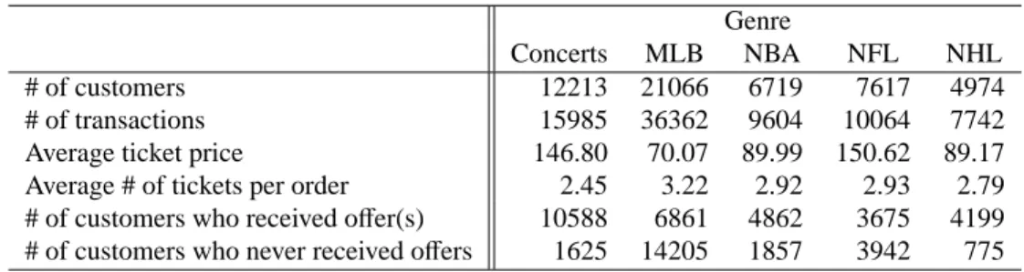
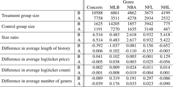
customers. Each transaction record includes customer ID, purchase time, event, number of tickets, and ticket price. Additional information about the customers includes their zip codes, genre pref-erences, and email preference. A customer has the option to opt out of email communication. We include only opted-in customers accounting for 45.7% of the customers in our data set. Table 1 provides key summary statistics for the five major genres with a total of 79,757 transactions. The data also exhibits cross-genre purchasing behavior of the customers. Numbers of customers who
have purchased two, three, four, and five different genres are 5,319, 996, 209, and 28, respectively,
representing 14.7% of all customers.
When launching an offer campaign, the company intended to target at a specific group of
tomers and randomly assigned customers from the group to treatment or control group. However, the data reveals that the randomized design was not properly implemented: customers in the
treat-ment and control groups differ significantly and the sizes of treatment and control groups of each
campaign are severely imbalanced (with control groups having fewer than 200 customers while
treatment groups having 2∼3,000 customers). As a remedy, we define a treatment group to include
all customers who received offers from the company during the time period under consideration,
whereas all other opted-in customers belong to the corresponding control group. In order to ensure the robustness of statistical inference to model misspecification, we match customers in the two groups to improve covariate balance so that the resulting data set resembles one generated from a properly randomized experiment (Imbens and Rubin, 2015).
Customer behavior, including customers’ transaction records, responses to marketing activi-ties, and Internet browsing records are commonly used in quantitative models for direct marketing (Venkatesan et al., 2007). It has also been shown that customers’ cross-genre purchasing behavior is an important aspect of customer relationship management (Ngobo, 2001; Kumar et al., 2008). Hence, given literature support and data availability, we use four main aspects of customer behav-ior as covariates in our analysis: (1) length of shopping history, which measures the length of time since a customer’s first purchase; (2) average price of tickets purchased, which suggests whether a customer is a value- or budget-customer; (3) average number of tickets per order, which indi-cates the size of group with whom a customer usually attends events; and (4) number of genres purchased, which captures a customer’s cross-genre purchasing behavior. We employ a propensity score matching approach by modeling treatment status as a logistic function of the four covariates (Rosenbaum and Rubin, 1985). The unit-matching approach consists of the following steps.
• Step 1: Estimate the propensity score of each customer, find the overlapping range R of
scores of treatment and control groups, and remove customers whose propensity scores lie
out of the range. Let Nt and Ncdenote the numbers of remaining customers in treatment and
control groups, respectively.
• Step 2: Stratify the range R into 5 strata and determine the maximum number of customers
from each group within each stratum under the constraint that the size ratio is Nt : NC.
Ran-domly select the determined number of customers from each group when needed. Combine
all the selected data.
As shown in Table 2, covariate imbalance has been significantly reduced for most of the co-variates after the matching. For the rest of the analysis, we use data of the matched groups and
consider that the two groups differ only in whether they have received an email offer from the
company. We also conducted the same analysis using all data without matching and the results were consistent with that from the matched data. Note that the full-data analysis is only valid if our specified analysis model is completely correct.
3
The Model For Purchase Events
3.1
Model formulation
Let ti j, i = 1,2, . . . ,I and j = 1,2, . . . ,Ni represent the time of the ith customer’s jth purchase.
We use a survival process to model each customer’s purchase history, in which a “death” event corresponds to a purchase. Conditioning on the previous transaction time, the occurrence of the
next purchase is governed by a hazard rate functionλi(t), so thatλi(t)Δt is the probability of having
the next purchase during the infinitesimal time period (t,t + Δt] conditional on having had no
purchases till time t. We emphasize that λi(t) is allowed to depend on all available information
up to time t, including the transaction time before. For simplicity, we omit all the conditioning
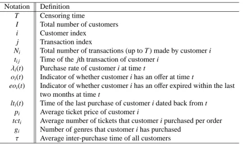
information in the notation of λi(t). Table 3 lists the main notations. Throughout the paper, we
use “hazard rate” and “purchase rate” interchangeably. Since each customer enters the company’s
database after his/her first purchase, we model subsequent transactions conditioning on the first one
by concatenating a series of survival processes. The occurrence of one purchase symbolizes the termination of the current process and initiation of a new one. All customers’ purchase processes
are censored at time T . Note that, ifR λi(t)dt is bounded, the probability that one will never make
another purchase is nonzero, and can be estimated from the data.
Conditioning on the time of the first purchase ti1 and the censoring time T , the probability
distribution function for intermediate purchases{ti j}Nj=i2 can be written as (Fleming and Harrington
(2011)): fi({ti j}Nj=i2|ti1,T )= exp − Z T ti1 λi(t)dt !YNi j=2 λi(ti j). (1)
When Ni =1, Equation (1) is reduced to only the exponential part. For simplicity, we suppress the
explicit dependence ofλi(t) on the purchase history before t.
As discussed in Section 1, survival process has been used in the marketing literature to model transaction data. These models usually allow the rate function to depend on covariates, but do not model seasonality explicitly. Our hazard function consists of three multiplicative components:
λi(t)=λ10(t)λ2i(t)λ3i(t), (2)
whereλ10(t) is a periodic function that depicts seasonality and serves as a baseline purchase rate,
λ2i(t) is an individual-specific factor that uses covariates to explain purchase rate, andλ3i(t) is the
random effects term that captures unobserved heterogeneity.
3.2
Three components of the purchase rate function
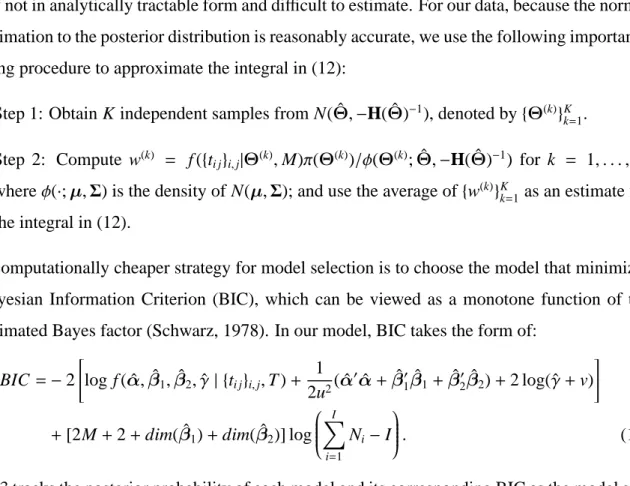
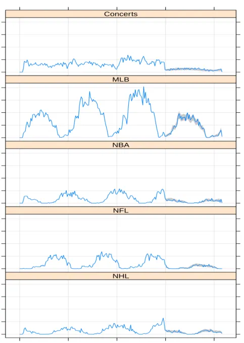
Seasonal effectλ10(t). Figure 1 plots the empirical purchase rates for the five genres that
demon-strate the need of a periodic function to model seasonality. These empirical purchase rates were estimated as follows. Each year was partitioned into 52 equal-length time window. For each
win-dow w of year n, we let Inwdenote the number of customers whose first purchase occurred before
the time window, and record ynw, the number of transactions made by those Inwcustomers during
this time window. Then the customers’ annual purchase rate for that time interval is estimated as
52(ynw/Inw). Its confidence interval can be obtained by assuming that ynwfollows a Poisson
distri-bution with the estimated purchase rate. Although less apparent for concerts, the sales of sports tickets display strong periodic patterns that match well with their corresponding sports seasons.
To reflect the strong seasonal effect, we letλ10(t) be a nonnegative periodic function that serves
as the baseline purchase rate for all customers. Since any periodic function can be approximated
well by its Fourier expansion up to M’th term, we expressλ10(t) as:
λ10(t)= max 0, α0+ M X m=1 [α2m−1sin(mωt)+α2mcos(mωt)] , (3)
whereωis 2πsince we use one year as the time unit for the function, and M typically ranges from 1 to 15, whose exact value will be determined by our full Bayesian model detailed in Section 4.2.
Although modeling logλ10(t) directly can ensure nonnegative rate, we choose the current form to
allowλ10(t) to be zero and for easier theoretical derivations.
Covariate effect λ2i(t). Taking into account the four covariates used for propensity score
matching and information about email offers, we postulate the following model to capture the
impact of customer characteristics and email offer on purchase rate:
logλ2i(t)= β1oi(t)+β2eoi(t)+β3(t−ti1)+β4(t−lti(t)−τ)+β5pi
+β6tcti+β7gi+β8oi(t)(t−ti1)+β9oi(t)(t−lti(t)−τ)
+β10oi(t)pi+β11oi(t)tcti+β12oi(t)gi, (4)
where oi(t) indicates whether customer i has a valid offer at time t, which reflects the immediate
offer effect, and eoi(t) indicates whether customer i has an offer that expired less than two months
ago at time t , which reflects the longer term effect of an offer. To avoid double-counting of offer
exposure, we set eoi(t) =0 when oi(t)=1.
β3captures the effect of shopping history. lti(t) is the time of customer i’s most recent purchase
andτ is the average interpurchase time of all customers up to time t, which will be estimated by
the sample mean a priori. There are two reasons for subtractingτfrom t to centralize the term
rep-resenting recency. First, it reduces the collinearity between main effect terms and their interaction
terms to almost zero. Second, after subtractingτ,β1 reflects the “average” offer effect, whereasβ9
represents additional offer effect when a customer’s purchase recency is distinct from the
popula-tion average. Nonlinear relapopula-tionship between recency and purchase rate has been examined in the literature. For example, Gonul and Shi (1998) and Gonul and Hofstede (2006) include a quadratic and a logarithmic term of recency, respectively. Our preliminary analysis showed that such nonlin-ear terms were insignificant and added computational burden substantially. Therefore, only linnonlin-ear
effect of recency is considered in the model. β5,β6, andβ7 represent the effects of average ticket
prices, average ticket count per order, and cross-genre purchase on purchase rate, respectively. β8
toβ12are the coefficients of the interaction terms that indicate the types of customers who are more
responsive to promotional offers.
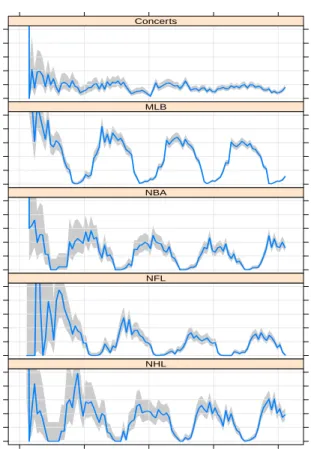
Random effectsλ3i(t). Figure 2 shows distributions of inter-purchase time for the five genres,
all exhibiting a wide range of values. A random effects term, λ3i(t), is necessary for capturing
unobserved heterogeneity among customers, which may include age, gender, income level,
occu-pation, marriage status, etc. We assume thatλ3i(t) is person-specific and time-invariant and will be
estimated from the data:λ3i(t)= δi.
4
Posterior Inference With the Model
4.1
The posterior distribution and marginalization
Functions oi(t) and eoi(t) in λ2i(t) are step functions of t. Their switching points, together with
purchase time {ti j}Nj=i1, partition the entire shopping history of customer i into a set of disjoint
intervals, denoted by Li1,Li2, . . . ,LiSi, where Si is the total number of such intervals of customer i
and∪Si
s=1Lis=[ti1,T ). Within each interval Lis, time of the last purchase, offer status, and post-offer
status are all constants. Let btis, etis, ltis, ois, and eois denote the beginning time (left boundary),
ending time (right boundary), last purchase time, offer status, and post-offer status associated with
interval Lis, respectively.
Within time interval Lis = [btis,etis), we replace time of the last purchase, offer status, and
post-offer status in Equation (4) by their corresponding interval-specific constants. Equation (4)
can be rewritten as
logλ2i(t)= β1ois+β2eois+β3(ltis−ti1+τ)+β5pi+β6tcti+β7gi+β8ois(ltis−ti1+τ)
+β10oispi+β11oistcti+β12oisgi+(β3+β4)(t−ltis−τ)
+(β8+β9)ois(t−ltis−τ). (5) More succinctly, we have
logλ2i(t)=Yis0β1+Zis0β2(t−ltis−τ)
for customer i at t∈Lis, and the customer’s overall purchase rate for t∈Lisis:
λis(t)≡ λi(t)|{t∈Lis} =max(0,X(t)
0α) exp(Y0
isβ1+Zis0β2(t−ltis−τ))δi, (6)
whereα= (α0, α1, . . . , α2M)0, β1 = (β1, β2, β3, β5, β6, β7, β8, β10, β11, β12)0,β2 = (β3+β4, β8+β9)0,
and
X(t)=(1,sin(ωt),cos(ωt), . . . ,sin(Mωt),cos(Mωt))0,
Yis=(ois,eois,ltis−ti1+τ,pi,tcti,gi,ois(ltis−ti1+τ),oispi,oistcti,oisgi)0,
Zis=(1,ois)0.
Using si j to index the unique interval among{Lis}sS=i1that covers transaction time ti j, i.e., ti j ∈Lisi j,
we can write the likelihood function for customer i as:
fi({ti j}Nj=i2|ti1,T )=exp − Si X s=1 Z Lis λis(t)dt Ni Y j=2 λisi j(ti j). (7)
In light of the left-skewedness of the log-inter-purchase time distributions shown in Figure 2,
we assume that random effectsδi’s follow a Gamma distribution and are independent of each other
a priori:
δi iid
∼ Gamma(γ, γ), i=1, . . . ,I. (8)
This distribution has mean 1 and variance 1/γ, implying that the random effect does not impact
the expected purchase rate but contributes to the population variance. Another advantage of the
Gamma prior is that it enables us to integrate out δi analytically.We assume that π(γ) ∝ (γ +
v)−21
γ>0.
We further assume a Gaussian prior for other parameters: (α,β1,β2)T ∼ N(0,u2I).
Hyper-parameters u=100 and v=1 are so chosen that the prior distributions are sufficiently diffuse, making
the inference sufficiently dependent on data. Combining the likelihood function and the priors, the
posterior distribution of all parameters of interest is: log f (α,β1,β2, γ,{δi}iI=1 | {ti j}i,j,T )= −α0 I X i=1 δi Si X s=1 exp(Yis0β1) Ais(Zis0β2)− Ris X r=1 ˜ Aisr(α,Zis0β2) + I X i=1 Ni X j=2 log(X(ti j)0α)+ I X i=1 Ni X j=2 Yis0i j β1+ I X i=1 Ni X j=2 Zis0i j(ti j−ltisi j) β2 + I X i=1 (Ni−1) log(δi)− 1 2u2(α 0α+β0 1β1+β20β2)+(γ−1) I X i=1 log(δi) −γXI
i=1δi+Iγlog(γ)−I logΓ(γ)−2 log(γ+v)+Const (9)
Integrating out all {δi}Ii=1 yields the posterior distribution of main parameters of interest that has
much lower dimensions:
log f (α,β1,β2, γ| {ti j}i,j,T )= − I X i=1 (Ni+γ−1) log γ+α0 Si X s=1 exp(Yis0β1) Ais(Zis0β2)− Ris X r=1 ˜ Aisr(α,Zis0β2) + I X i=1 Ni X j=2 log(X(ti j)0α)+ I X i=1 Ni X j=2 Yis0i j β1+ I X i=1 Ni X j=2 Zis0i j(ti j−ltisi j) β2 − 1 2u2(α 0α+β0 1β1+β20β2) +XI
i=1logΓ(Ni+γ−1)+Iγlog(γ)−I logΓ(γ)−2 log(γ+v)+Const (10)
4.2
Bayesian computation via Markov chain Monte Carlo
To draw inferences, we implement a Markov chain Monte Carlo (MCMC) algorithm to sample
from the posterior distribution f (Θ). In order to improve computational efficiency, we first use a
modified Newton-Raphson algorithm to find the posterior mode ˆΘand the corresponding inverse
Hessian matrix H( ˆΘ)−1 (see Appendix 7.3 for details). We then initialize the sampler withΘ(0) =
ˆ
Θand implement a random-walk Metropolis (RWM) algorithm (Liu, 2008): At step t+1, generate
Θ(t+1)
prop =Θ
(t)
+, where ∼ N0,−σ2
H( ˆΘ)−1, (11)
then let Θ(t+1) = Θ(t+1)
prop with probability pa ≡ min
n
1, f (Θ(tprop+1))/f (Θ(t)) o
and Θ(t+1) = Θ(t) with
probability 1− pa.
Importance sampling and independent Metropolis-Hastings (IMH) algorithm can take advan-tage of Normal approximation to the posterior distribution as well (Liu, 1996, 2008). However, even when normal approximation is reasonably close to the true posterior, the RWM proposal de-scribed by (11) can still lead to very sticky algorithm in high-dimensions, and the corresponding importance sampling and IMH algorithms can only be worse – leading to unstable approximations (Liu, 1996). A good alternative is to combine Gibbs sampling with Metropolis type moves, es-pecially given that we have observed from the inverse-Hessian matrix that no pair of parameters
are too highly correlated. More precisely, since Θ can be represented as {α,β1,β2, γ}, we
cy-cle through each of the four elements with conditional updates, i.e., updating Θd by draws from
f (Θd |Θ(t)[−d]) for d = 1,2,3,4. Although at a lower dimension, each conditional distribution still
evades exact sampling. We thus make l=10 steps of RWM moves within each conditional move,
with the proposal covariance matrix beingΣd =2.382(−Hdd)−1/dim(Θd), where Hdd stands for the
sub-matrix of H corresponding toΘd. The step size was recommended by Gelman et al. (1996)
for Gaussian-like target distributions to achieve maximum efficiency. As shown in Section 5, for
our data set the posterior samples obtained by the MCMC strategy coincide very well with the asymptotic normal distribution derived in the Supplementary Materials.
4.3
Bayesian model selection
As discussed in Section 3.2, we model the baseline hazard as a periodic function with M Fourier expansion terms. To find a proper M for each genre, we employ a Bayesian model selection
strategy in which we give each model a prior, compute model likelihood (i.e., P(data | M), where
M represents a model), and choose the model with the highest posterior probability. The posterior
probability of a model M can be written as
p(M|{ti j}i,j)∝ p0(M)
Z
f ({ti j}i,j|ΘM,M)π(ΘM)dΘM, (12)
where p0(M) is a prior belief of M that is assumed to be uniform.
The model likelihood, also known as the normalizing constant for the posterior distribution, is
usually not in analytically tractable form and difficult to estimate. For our data, because the normal approximation to the posterior distribution is reasonably accurate, we use the following importance sampling procedure to approximate the integral in (12):
• Step 1: Obtain K independent samples from N( ˆΘ,−H( ˆΘ)−1), denoted by{Θ(k)}K
k=1.
• Step 2: Compute w(k) = f ({t
i j}i,j|Θ(k),M)π(Θ(k))/φ(Θ(k); ˆΘ,−H( ˆΘ)−1) for k = 1, . . . ,K,
whereφ(∙;μ,Σ) is the density of N(μ,Σ); and use the average of{w(k)}kK=1as an estimate for
the integral in (12).
A computationally cheaper strategy for model selection is to choose the model that minimizes the Bayesian Information Criterion (BIC), which can be viewed as a monotone function of the approximated Bayes factor (Schwarz, 1978). In our model, BIC takes the form of:
BIC=−2 " log f ( ˆα,βˆ1,βˆ2,γˆ | {ti j}i,j,T )+ 1 2u2( ˆα 0αˆ +βˆ0 1βˆ1+βˆ20βˆ2)+2 log( ˆγ+v) #
+[2M+2+dim( ˆβ1)+dim( ˆβ2)] log
I X i=1 Ni−I . (13)
Figure 3 tracks the posterior probability of each model and its corresponding BIC as the model size grows. The two model selection criteria clearly agree on the same optimal model for all genres except NFL, whose optimal and sub-optimal models are however quite close in terms of either criterion. For concerts, the optimal M is found at 1, which is consistent with the fact that the periodic pattern of concert ticket sales is the weakest among the five genres. MLB requires a much
larger M (M =10), while the other three genres all favor a moderate M of around 5.
4.4
Prediction of future events
Predicting customers’ future purchase behavior is of practical interest of the company. Specifically, given customer l’s purchase history up to time T , we want to forecast the number of orders that she
will place in the nextΔT years. It can be answered via Monte Carlo simulation of her purchases
during (T,T+ΔT ] given that her offer status during (T,T+ΔT ] is known. First we sample{Θ(k)}K
k=1
as described in Section 4.3 using the MCMC algorithm. For each k, we drawδ(k)l from Gamma(Nl+
γ(k)−1,(α(k))0PSl
s=1B (k)
is +γ
(k)) and sample new purchases iteratively. Given the customer’s latest
transaction time tl j (either recorded or sampled) for the period (tl j,min{T + ΔT,tl,j+1}], we can construct intervals {L( j)ls}S ( j) l s=1 and {L˜ ( j)(α(k))} ls} S( j)l s=1, and vectors Y ( j) ls and Z ( j)
ls in the same way as
described before. The next purchase time tl,j+1is governed by the hazard rate:
λ(k j)ls (t)= max(0,X(t)0α(k)) exp((Y( j) ls )0β (k) 1 +(Z ( j) ls )0β (k) 2 (t−tlNl −τ))δ (k) l .
The process of tl,j+1can be simulated accordingly. An algorithm to sample from a survival process
with an inhomogeneous hazard rate is provided by Cinlar (2013). Every time after a new purchase time is sampled, the rate function is updated by treating the current purchase as the last purchase input for the new process. We repeat the procedure until the newest sampled purchase time
sur-passes T + ΔT . Then we estimate the expected sales by taking the average of the resulting number
of purchases for each simulated process. The prediction result is discussed in Section 5.3.
5
Results and Interpretations
5.1
O
ff
er e
ff
ects
Employing the model discussed in Section 3, we assess the effects of email offer, customer
char-acteristics, and their interactions on customers’ purchase rate of event tickets. Table 4 summarizes
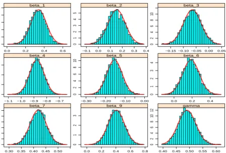
posterior means and standard deviations for coefficients of interest for the five genres. Figure 4
shows histograms of posterior samples obtained via the MCMC algorithm described in Section 4.2 overlaid with their normal approximations.
NHL goers appear to be the most responsive to promotional offers. On average, an offer
in-creases the purchase rate of NHL tickets by 34.0% and 15.3% in the short and long terms,
re-spectively. The purchase rate of NFL tickets increases by 24.2% when an offer is valid; while the
purchase rate of MLB tickets increases by 17.2% during the two months after a customer receives
an offer. Although the promotional offers do not show significant immediate effect on genres other
than NFL and NHL, the data reveal that the offer campaigns launched by the company did
suc-cessfully promote sales to some extent. It is worth noting that the offers exhibit long-term effect
as well, i.e., the customer purchase rate is elevated even after an offer expires. This may be due to
the situation where a customer does not have an immediate need to buy tickets, but receiving an
offer reminds the customer about the company and then the customer recalls and purchases from it when a need arises. The company can benefit from such behaviors because it increases purchase rate without compromising the profit margin.
We also investigate interactions between the promotional offer and customer characteristics.
Except the one between offer and recency, we do not discover other significant interactions. A
positive interaction exists between offer and recency for NBA and NHL. NHL has shown positive
immediate and long-term effects of promotional offers. This positive interaction further reveals
that customers who have been inactive for a while are more inclined to take advantage of an offer.
When recency is large, offers serve as an effective catalyst for attracting customers back to make a
purchase.
5.2
Customer characteristics e
ff
ects
Customer characteristics have some interesting impacts on purchase rate. Length of shopping his-tory, defined as the length of time from a customer’s first purchase until the time point under con-sideration, has a negative impact on the purchase rates of all genres except concerts. For instance,
the purchase rate of an MLB ticket buyer decreases by 1−exp(−0.041)= 4.0% each year from the
time she joins the company when the other covariates stay unchanged. The percentage decreases
are 10.9%, 9.2% and 6.3% for NBA, NFL and NHL, respectively. The result suggests that
cus-tomers lose interest in purchasing from the company over time. Recency, defined as time elapsed since the last purchase, has been studied extensively in the literature and is shown to be a good predictor of customers’ purchase behavior (Elsner et al. (2004)). For regularly-consumed
prod-ucts, such as clothes, food, and office supplies, empirical data showed that customers with smaller
recency are more likely to respond to marketing activities, i.e., recency has a negative impact on response rate (e.g., Bitran and Mondschein (1996), Gonul and Shi (1998)). This phenomenon can be explained by the dynamics that when considering frequently-purchased products, the fact that a customer does not buy in a period time usually means that she is buying elsewhere. The longer the time a customer has not purchased from a company, the lower the probability that she will
come back to the company. On the other hand, positive effect of recency is observed as well. For
example, the purchase probability of durable goods may increase with recency because consumers
need to replace their product when approaching the end of the product’s life cycle (e.g., Roberts
and Berger (1989) and Ansari et al. (2008)). Our result shows that recency negatively affects the
purchase rates of all genres. It suggests that in terms of recency’s impact, event ticket purchase resembles the behavior of frequently-purchased products, although its purchase frequency is much lower. In essence, the likelihood of a customer making another purchase decreases as time passes.
This, along with the effect of the length of shopping history, makes customer retention a
challeng-ing task for the company, which in fact validates the company’s concern over it. In order to keep customers interested and active, the company needs to engage customers as early and frequent as possible by using a variety of marketing activities.
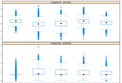
Average ticket price significantly affects the purchase rate of all genres except NBA. However,
the signs are inconsistent: it is positive for concerts and NFL, while negative for MLB and NHL.
The opposite signs may be explained by the price level and fan base of different genres. Figure 5
provides box plots showing the differences in average ticket prices of the five genres. Also as shown
in Table 1, the average ticket prices of concerts and NFL are $146.80 and $150.62, respectively, while those of MLB and NHL are $70.07 and $89.17, respectively. The result indicates that at a higher price level, customers who buy more expensive tickets tend to buy more often; while at a lower price level, it is the opposite: customers who buy cheaper tickets tend to buy more often.
The effect of average ticket count per order on purchase rate is significant for all genres, except
concerts. The signs are also mixed: NBA, NFL, and NHL have positive coefficients, while MLB
has a negative one. The former three genres have smaller average ticket count per order (2.92, 2.93, and 2.79, respectively) than MLB (3.22), which is statistically significant (see Figure 5). In
essence, when ticket count per order is small, purchase rate increases with ticket count; the effect
reverses when ticket count is large. Notably low ticket count per order may imply that a person attends an event alone to try it out. An increasing ticket count suggests that a stable group of people attend events together, which tend to make it a more regular activity. When ticket count is considerably high, it may indicate a one-time gathering with a large group which does not happen often. This implies that there is a certain range of average ticket count that leads to the highest purchase rate.
Summarizing the effects of average ticket price and average ticket count per order by genre
provides useful insights on customer segmentation. For concerts and NFL, characterized by high ticket price and low ticket count per order, customers who highly value good seats (reflected by more expensive tickets) and attend with a relatively large group (reflected by higher ticket count per order) are the ones who have high purchase rate, which may be the most valuable customers to the company. These customers are devoted fans to the genre who are likely to enjoy it with their
family and/or close friends. For MLB, characterized by low ticket price and high ticket count per
order, its customers exhibit opposite behavior: the ones who buy cheaper tickets and attend with a relatively small group tend to purchase more frequently. This seems to suggest that people who enjoy MLB games as a small-scale social event (evidenced by attending with an extended, but not too large, group of family and friends) and do not care too much about having good seats, tend to go more often. Lastly, for NBA and NHL, characterized by low ticket price and low ticket count per order, customers who buy less expensive tickets and attend with a larger group are likely to purchase frequently.
Number of genres that a customer has purchased from the company represents the degree of cross-buying of the customer, which has been associated with higher levels of customer reten-tion, revenue generareten-tion, and loyalty (Reinartz et al. (2008)). Our result clearly shows that as the purchased number of genres increases, purchase rate increases for all five genres. It is consistent with the findings in the literature and accentuates the importance of promoting cross-selling to the company. Although the observed association may not imply causation, it is worthwhile for the company to send targeted informational or promotional emails introducing multiple genres to a new customer to raise her awareness and stimulate cross-buying behavior.
5.3
Prediction results
To validate model fitting and illustrate the prediction power of our proposed model, we choose an
intermediate time point t0 and use transaction records prior to t0 to predict transactions occurred
after it. We set t0 to be January 1, 2010. Figure 6 illustrates the comparison between our model
prediction and the actual sales for the five genres. The apparent shape difference between training
and test periods is because only existing customers’ purchases are predicted during the test period. We evaluate the prediction accuracy by root mean squared errors (RMSE) of the total predicted
sales on the logarithm scale during the test period, which is calculated as: RMS E = v t 1 H H X h=1 (log pcd (h)−log pc)2
where log pcd (h) = PKk=1log pcd (hk)
/n and pc is the actual purchase count during the test period.
That is, we replicate H independent predictions of log-purchase count and each predictionlog pcd (h)
is estimated by the average of K simulated purchase counts as explained in Section 4.4 (aggregated
over all customers and on the logarithmic scale). RMSEs with K =1000 for concerts, MLB, NBA,
NFL, and NHL are 0.134, 0.071, 0.104, 0.048 and 0.057, respectively, which indicates satisfactory prediction capability.
6
Concluding Remarks
We have employed the survival analysis framework developed in biostatistics and adopted recently by marketing researchers to model recurring purchase events and to examine how email marketing
campaigns and personal characteristics affect customers’ purchasing behaviors. Our model is a
generalized proportional hazard model that enables us to accomplish two goals. First is to connect an individual customer’s purchase likelihood to a variety of factors, including customer character-istics and marketing variables. Second is to predict future purchases made by existing customers
based on their historical transactions and email offer information.
In our Bayesian model, a customer’s purchase rate is characterized by a hazard rate function consisting of three components: a baseline function, a function of covariates, and a random
ef-fect term capturing unobserved heterogeneity. Different from existing models in the literature, for
the baseline function, we postulate a periodic function to model the seasonality of event ticket purchases. Our approach is fully Bayesian, making the inference less dependent on asymptotic approximations. We are able to analytically integrate over the hazard rate function and the random
effects so as to derive a workable posterior distribution with much lower dimensions, for which
both a Newton-Raphson mode-finding algorithm and an efficient MCMC algorithm are
imple-mented. Another attractive aspect of our Bayesian approach is that it can be conveniently used to provide purchase predictions via Monte Carlo simulations.
Our results reveal that email offers have different degrees of effectiveness for different event
genres. Therefore, a one-size-fits-all email marketing strategy is unlikely to be effective. Instead,
the use of genre-specific offers should be encouraged and explored. The effects of email offers,
purchase recency, and their positive interaction suggest that there is an optimal timing for using
offers to revive inactive customers. Examining the impact of average ticket price and average
ticket count per order on purchase rate allows customer segmentation based on the two factors.
Email offers can then be used to shape customer behavior and habit into the types that are the most
valuable to the company.
7
Appendix
7.1
Deriving the log-likelihood function
Define D(α) = {t ∈ (−∞,∞) : X(t)0α <= 0}. The region D(α)∩[ti1,T ) can be decomposed
into Ri disjoint sets{L(˜ α)is}Ss=i1 where ˜L(α)is = D(α)∩Lis. The boundary points of ˜L(α)is are
either ones of Lisor roots of the equationX(t)0α=0 within [ti1,T ). Apparently values of the offer
status, post-offer status and last purchase time within ˜L(α)isremain the same of those of Lis.
It is easy to see that ˜L(α)is is a set of disconnected intervals (also can be empty set). Let
˜
L(α)is= ∪Rr=is1[ ˜bt(α)isr,et(˜ α)isr].
Expand the exponent part of equation (7). Si X s=1 Z Lis λis(t)dt= Si X s=1 Z Lis max(0,X(t)0α) exp(Yis0β1+Zis0β2(t−ltis−Δt))δidt = Si X s=1 Z Lis X(t)0αexp(Yis0β1+Zis0β2(t−ltis−Δt))δidt − Si X s=1 Z ˜ L(α )is X(t)0αexp(Yis0β1+Zis0β2(t−ltis−Δt))δidt = δi hXSi s=1 Z etis btis X(t)0αexp(Yis0β1+Zis0β2(t−ltis−Δt))dt − Si X s=1 Ris X r=1 Z et(˜ α )isr ˜ bt(α )isr X(t)0αexp(Yis0β1+Zis0β2(t−ltis−Δt))dt i
The integration ofλis(t)dt over interval [a,b] is
Z b a λis(t)dt = Z b a δiexp(Yis0β1)α0X(t) exp(Zis0β2(t−ltis−Δt))dt =δiexp(Yis0β1)α0 Z b a X(t) exp(Zis0β2(t−ltis−Δt))dt =δiexp(Yis0β1)α0 Z b−ltis−Δt a−ltis−Δt X(t+ltis+ Δt) exp(Zis0β2t)dt
Define Aba(ω, φ, θ)= Z b a sin(ωt+φ) exp(θt)dt = (b1−a) sinφ ifω=θ= 0 θ2+ω2 θsin(ωt+φ)−ωcos(ωt+φ) exp(θt)bt=a otherwise And define Ais(θ)= Aetis−ltis−Δt btis−ltis−Δt (0, π/2, θ), Aetis−ltis−Δt btis−ltis−Δt (ω, ω∙(ltis+ Δt), θ),Abtetis−ltis−Δt is−ltis−Δt (ω, ω∙(ltis+ Δt)+π/2, θ), Aetis−ltis−Δt btis−ltis−Δt (2ω,2ω∙(ltis+ Δt), θ),Aetis−ltis−Δt btis−ltis−Δt (2ω,2ω∙(ltis+ Δt)+π/2, θ), ∙ ∙ ∙ , Aetis−ltis−Δt btis−ltis−Δt (Mω,Mω∙(ltis+ Δt), θ),Aetis−ltis−Δt btis−ltis−Δt (Mω,Mω∙(ltis+ Δt)+π/2, θ) 0 ˜ Aisr(α, θ)= Aet(˜ α )isr−ltis−Δt ˜ bt(α )isr−ltis−Δt (0, π/2, θ), Aet(˜ α )isr−ltis−Δt ˜ bt(α )isr−ltis−Δt (ω, ω(ltis+ Δt), θ),A ˜ et(α )isr−ltis−Δt ˜ bt(α )isr−ltis−Δt (ω, ω(ltis+ Δt)+π/2, θ), Aet(˜ α )isr−ltis−Δt ˜ bt(α )isr−ltis−Δt (2ω,2ω(ltis+ Δt), θ),A ˜ et(α )isr−ltis−Δt ˜ bt(α )isr−ltis−Δt (2ω,2ω(ltis+ Δt)+π/2, θ), ∙ ∙ ∙ , Aet(˜ α )isr−ltis−Δt ˜ bt(α )isr−ltis−Δt (Mω,Mω(ltis+ Δt), θ),A ˜ et(α )isr−ltis−Δt ˜ bt(α )isr−ltis−Δt (Mω,Mω(ltis+ Δt)+π/2, θ) 0
We obtain a simplified form of log fi:
log fi({ti j}Nj=i2|α,β1,β2, γ,{δi}iI=1,ti1,T )= −δiα0 Si X s=1 exp(Yis0β1) Ais(Zis0β2)− Ris X r=1 ˜ Aisr(α,Zis0β2) + Ni X j=2 log(X(ti j)0α)+ Ni X j=2 Yis0i j β1+ Ni X j=2 Zis0i j(tij−ltisi j) β2 +(Ni−1) log(δi)
Aggregating log fi for all i’s yields the total density function for all observations. log f ({ti j}Nj=i2iI=1α,β1,β2, γ,{δi}iI=1,T )= −α0 I X i=1 δi Si X s=1 exp(Yis0β1) Ais(Zis0β2)− Ris X r=1 ˜ Aisr(α,Zis0β2) + I X i=1 Ni X j=2 log(X(ti j)0α)+ I X i=1 Ni X j=2 Yis0i j β1+ I X i=1 Ni X j=2 Zis0i j(ti j−ltisi j) β2 + I X i=1 (Ni−1) log(δi)
7.2
Gradient and Hessian matrix of the log-posterior
Gradient: ∇log f = ∂log f
∂α , ∂log f ∂β1 ,∂log f ∂β2 ,∂log f ∂γ ! , Hessian Matrix: H= ∂2log f ∂α ∂α 0 ∂2log f ∂α ∂β 01 ∂2log f ∂α ∂β 02 ∂2log f ∂α ∂γ ∂2log f ∂β 1∂α 0 ∂2log f ∂β 1∂β 01 ∂2log f ∂β 1∂β 02 ∂2log f ∂β 1∂γ ∂2log f ∂β 2∂α 0 ∂2log f ∂β 2∂β 01 ∂2log f ∂β 2∂β 02 ∂2log f ∂β 2∂τ ∂2log f ∂γ∂α 0 ∂2log f ∂γ∂β 10 ∂2log f ∂γ∂β 20 ∂2log f ∂γ∂γ . Define Bis =exp(Yis0β1) Ais(Zis0β2)− Ris X r=1 ˜ Aisr(α,Zis0β2) , Bis(1) =exp(Yis0β1) ∂∂θAis(Zis0β2)− Ris X r=1 ∂A˜isr ∂θ (α,Z 0 isβ2) , Bis(2) =exp(Yis0β1) ∂ 2A is ∂θ2 (Z 0 isβ2)− Ris X r=1 ∂2A˜ isr ∂θ2 (α,Z 0 isβ2) .
Then ∂log f ∂α =− I X i=1 (Ni+γ−1)PSs=i1Bis γ+α0PSi s=1Bis + I X i=1 Ni X j=2 X(ti j) X(ti j)0α − α u2 ∂log f ∂β1 =− I X i=1 (Ni+γ−1)α0PSs=i1BisYis γ+α0PSi s=1Bis + I X i=1 Ni X j=2 Yisi j− β1 u2 ∂log f ∂β2 =− I X i=1 (Ni+γ−1)α0PSs=i1B (1) is Zis γ+α0PSi s=1Bis + I X i=1 Ni X j=2 Zis0i j(ti j−ltisi j)− β2 u2 ∂log f ∂γ =− I X i=1 log γ+α0 Si X s=1 Bis − I X i=1 Ni+γ−1 γ+α0PSi s=1Bis +XI i=1ϕ(Ni+γ−1)−Iϕ(γ)+I log(γ)+I− 2 γ+v,
whereϕ(x)= d logdxΓ(x) is the digamma function.
∂2log f ∂α∂α0 =− I X i=1 (Ni+γ−1) " 1 γ+α0PSi s=1Bis ∙ Si X s=1 X r:α 0X( ˜et(α )isr)=0
exp(Yis0β1+( ˜et(α)isr −ltis−Δt)Zis0β2)
α0∂X
∂t ( ˜et(α)isr)
X( ˜et(α)isr)X( ˜et(α)isr)0
− Si X s=1 X r:α 0X( ˜bt(α )isr)=0 exp(Yis0β1+( ˜bt(α)isr−ltis−Δt)Zis0β2) α0∂X ∂t ( ˜bt(α)isr) X( ˜bt(α)isr)X( ˜bt(α)isr)0 ! − PSi s=1Bis γ+α0PSi s=1Bis PSi s=1Bis γ+α0PSi s=1Bis 0# − I X i=1 Ni X j=2 X(ti j)X(ti j)0 X(ti j)0α 2 − 1 u2Idim(α ) ∂2log f ∂β1∂β10 =− I X i=1 (Ni+γ−1) α0PSi s=1BisYisYis0 γ+α0PSi s=1Bis − α0 PSi s=1BisYis γ+α0PSi s=1Bis α0PSi s=1BisYis γ+α0PSi s=1Bis 0 − 1 u2Idim(β 1) ∂2log f ∂β2∂β20 =− I X i=1 (Ni+γ−1) α0PSi s=1B (2) is ZisZis0 γ+α0PSi s=1Bis − α0 PSi s=1B (1) is Zis γ+α0PSi s=1Bis α0PSi s=1B (1) is Zis γ+α0PSi s=1Bis 0 − u12Idim(β 2)
∂2log f ∂γ∂γ =− I X i=1 γ+α0P2Si s=1Bis − Ni+γ−1 γ+α0PSi s=1Bis 2 + I X i=1 ϕ1(Ni+γ−1)−Iϕ1(γ)+ I γ + 2 (γ+v)2
whereϕ1(x)= dϕdx(x) is the trigamma function.
∂2log f ∂α∂β10 =− I X i=1 (Ni+γ−1) PSi s=1BisYis0 γ+α0PSi s=1Bis − PSi s=1Bis γ+α0PSi s=1Bis α0PSi s=1BisYis γ+α0PSi s=1Bis 0 ∂2log f ∂α∂β20 =− I X i=1 (Ni+γ−1) PSi s=1B (1) is Zis0 γ+α0PSi s=1Bis − PSi s=1Bis γ+α0PSi s=1Bis α0PSi s=1B (1) is Zis γ+α0PSi s=1Bis 0 ∂2log f ∂α∂γ − I X i=1 PSi s=1Bis γ+α0PSi s=1Bis − (Ni+γ−1) PSi s=1Bis γ+α0PSi s=1Bis 2 ∂2log f ∂β1∂β20 =− I X i=1 (Ni+γ−1) α 0PSi s=1BisYisZis0 γ+α0PSi s=1Bis − α 0PSi s=1BisYis γ+α0PSi s=1Bis α 0PSi s=1BisZis γ+α0PSi s=1Bis 0 ∂2log f ∂β1∂γ =− I X i=1 α 0PSi s=1BisYis γ+α0PSi s=1Bis − (Ni+γ−1)α0 PSi s=1BisYis γ+α0PSi s=1Bis 2 ∂2log f ∂β2∂γ =− I X i=1 α 0PSi s=1B (1) is Zis γ+α0PSi s=1Bis − (Ni +γ−1)α0 PSi s=1B (1) is Zis γ+α0PSi s=1Bis 2
7.3
Posterior mode finding and normal approximation
LetΘ= {α,β1,β2, γ}. For convenience, we abbreviate the posterior distribution in (10) as f (Θ).
Note that log f (Θ) is differentiable everywhere and twice-differentiable almost everywhere. We
thus adopt a modified Newton-Raphson (NR) algorithm with adaptive step-size in each iteration so as to avoid the chaotic behavior of the classic NR update (Amrein and Wihler (2014)). Formulas for the gradient and Hessian matrix of (10) are provided in Appendix 7.2.
We initialize β1 andβ2with vectors of zeros, andγwith a small value, say 0.01, to allow for
a large heterogeneity. The initial value of the seasonal effectα is most crucial, and is set to be
a preliminary estimate from the following procedure, which applies the Fourier transform to an
empirically estimated purchase rate function:
1. Partition each year into W = 52 equal-length time windows. With a simple Poisson model,
we estimate the average purchase rate ˆμwof the wth interval as Wyw/Iwand its standard error
s( ˆμw) as W√yw/Iw, where yw is the total number of purchases that occurred within the wth
interval of all years and Iw the number of potential buyers aggregating over all years for that
interval. The empirical purchase rate function ˆP(t) is estimated as being equal to ˆμw in the
wth time window of the year.
2. Compute the Fourier transform of the empirical purchase rate function to obtain: ˆ α0 = PW w=1μˆw/s( ˆμw)2 PW w=11/s( ˆμw)2 =W PW w=1Iw PW w=1Iw2/yw ˆ α2m−1 = 2W PW w=1Iw2/yw W X w=1 sin 2πmw−.5 W ! Iw, m= 1, . . . ,M; ˆ α2m = 2W PW w=1Iw2/yw W X w=1 cos 2πmw−.5 W ! Iw, m= 1, . . . ,M.
3. Check if the resulting ˆαsatisfiesX(ti j)0αˆ > 0 for all i and j’s. Otherwise, increase ˆα0 by
0.001−mini,jX(ti j)0αˆ to satisfy this requirement.
With these initial values, the modified NR algorithm converges typically in fewer than 20
iter-ations for all the five datasets. Around its mode ˆΘ, the posterior distribution f (Θ) can be
approxi-mated well by a normal distribution N( ˆΘ,−H( ˆΘ)−1) when sample size is large enough (O’Hagan
et al. (2004)), where H(Θ) is the Hessian matrix.
8
Supplemental Material
It details the MCMC posterior sampling procedures introduced in Section 4.2, together with the results for our ticket transaction data (a PDF file), available at the journal’s website.
References
Ailawadi, K. L. and Neslin, S. A. (1998). The effect of promotion on consumption: Buying more
and consuming it faster. Journal of Marketing Research, 35(3):390–8.
Allenby, G., Leone, R., and Jen, L. (1999). A dynamic model of purchase timing with application to direct marketing. Journal of the American Statistical Association, 94(446):365–74.
Amrein, M. and Wihler, T. P. (2014). An adaptive newton-method based on a dynamical systems approach. Communications in Nonlinear Science and Numerical Simulation, 19(9):2958–2973. Ansari, A., Mela, C., and Neslin, S. (2008). Customer channel migration. Journal of Marketing
Research, 45(February):60–76.
Bijwaard, G. E., Franses, P. H., and Paap, R. (2006). Modeling purchases as repeated events.
Journal of Business and Economic Statistics, 24(4):487–502.
Bitran, G. R. and Mondschein, S. V. (1996). Mailing decisions in the catalog sales industry.
Management Science, 42(9):1364–81.
Boatwright, P., Borle, S., and Kadane, J. (2003). A model of the joint distribution of purchase quantity and timing. Journal of the American Statistical Association, 98(463):564–72.
Bucklin, R. E. and Lattin, J. M. (1991). Two-state model of purchase incidence and brand choice.
Marketing Science, 10(1):24–39.
Chan, T., Narasimhan, C., and Zhang, Q. (2008). Decomposing promotional effects with a dynamic
structural model of flexible consumption. Journal of Marketing Research, 45(4):487–98. Chintagunta, P. and Haldar, S. (1998). Investigating purchase timing behavior in two related
prod-uct categories. Journal of Marketing Research, 35(1):45–53.
Chintagunta, P. K. (1993). Investigating purchase incidence, brand choice and purchase quantity decisions of households. Marketing Science, 12(2):184–208.
Cinlar, E. (2013). Introduction to stochastic processes. Courier Dover Publications.
Elsner, R., Krafft, M., and Huchzermeier, A. (2004). Optimizing rhenania’s direct marketing business through dynamic multilevel modeling (dmlm) in a multicatalog-brand environment.
Marketing Science, 23(2):192–206.
Fleming, T. R. and Harrington, D. P. (2011). Counting processes and survival analysis, volume 169. John Wiley & Sons.
Gelman, A., Roberts, G., and Gilks, W. (1996). Efficient metropolis jumping rules. Bayesian
Statistics 5, JM Bernardo, JO Berger, AP Dawid, and AFM Smith (eds), pages 599–607.
Gonul, F. and Shi, M. Z. (1998). Optimal mailing of catalogs: A new methodology using estimable structural dynamic programming models. Management Science, 44(9):1249–62.
Gonul, F. and Srinivasan, K. (1993). Consumer purchase behavior in a frequently bought product category. Journal of the American Statistical Association, 88(88):1219–27.
Gonul, F. F. and Hofstede, F. T. (2006). How to compute optimal catalog mailing decisions.
Marketing Science, 25(1):65–74.
Gupta, S. (1988). Impact of sales promotions on when, what, and how much to buy. Journal of
Marketing Research, 25(4):342–55.
Imbens, G. W. and Rubin, D. B. (2015). Causal Inference for Statistics, Social, and Biomedical
Sciences. Cambridge University Press.
Jain, D. and Vilcassim, N. J. (1991). Investigating household purchase timing decisions: A condi-tional hazard function approach. Marketing Science, 10(10):1–23.
Kamakura, W. and Kang, W. (2007). Chain-wide and store-level analysis for cross-category man-agement. Journal of Retailing, 83(2):159–70.
Kumar, V., George, M., and Pancras, J. (2008). Cross-buying in retailing: Drivers and conse-quences. Journal of Retailing, 84(1):15–27.
Liu, J. S. (1996). Metropolized independent sampling with comparisons to rejection sampling and importance sampling. Statistics and Computing, 6(2):113–119.
Liu, J. S. (2008). Monte Carlo strategies in scientific computing. Springer Science & Business Media.
Manchanda, P. J. D., Goh, K., and Chintagunta, P. (2006). The effect of banner advertising on
internet purchasing. Journal of Marketing Research, 43(1):98–108.
Ngobo, P. (2001). Drivers of customers’ cross-buying intentions. European Journal of Marketing,
38(9/10):1129–57.
O’Hagan, A., Forster, J., and Kendall, M. G. (2004). Bayesian inference. Arnold London.
Osinga, E. C., Leeflang, P. S., and Wieringa, J. E. (2010). Early marketing matters: A time-varying parameter approach to persistence modeling. Journal of Marketing Research, 47(February):173– 85.
Reinartz, W., Thomas, J. S., and Bascoul, G. (2008). Investigating cross-buying and customer loyalty. Journal of Interactive Marketing, 22(1):5–20.
Roberts, M. L. and Berger, P. D. (1989). Direct Marketing Management. Prentice-Hall, Inc,
Englewood Cliffs, New Jersey.
Rosenbaum, P. R. and Rubin, D. B. (1985). Constructing a control group using multivariate matched sampling methods that incorporate the propensity score. The American Statistician, 39(1):33–38.
Schwarz, G. (1978). Estimating the dimension of a model. The Annals of Statistics, 6(2):461–464. Seetharaman, P. B. and Chintagunta, P. K. (2003). The proportional hazard model for purchase timing: A comparison of alternative specifications. Journal of Business and Economic Statistics, 21(3):368–82.
VanBoskirk, S. Us interactive marketing forecast, 2007 to 2012. https://member-west.
express-scripts.com/images/pdf/Previewtest.pdf.