HAL Id: hal-00786098
https://hal-enpc.archives-ouvertes.fr/hal-00786098
Submitted on 12 Feb 2018HAL is a multi-disciplinary open access archive for the deposit and dissemination of sci-entific research documents, whether they are pub-lished or not. The documents may come from teaching and research institutions in France or abroad, or from public or private research centers.
L’archive ouverte pluridisciplinaire HAL, est destinée au dépôt et à la diffusion de documents scientifiques de niveau recherche, publiés ou non, émanant des établissements d’enseignement et de recherche français ou étrangers, des laboratoires publics ou privés.
Quantifying the impact of small scale unmeasured
rainfall variability on urban runoff through multifractal
downscaling: A case study
Auguste Gires, C. Onof, C. Maksimovic, D Schertzer, Ioulia Tchiguirinskaia,
N. Simoes
To cite this version:
Auguste Gires, C. Onof, C. Maksimovic, D Schertzer, Ioulia Tchiguirinskaia, et al.. Quantifying the impact of small scale unmeasured rainfall variability on urban runoff through multifractal downscaling: A case study. Journal of Hydrology, Elsevier, 2012, 442-443, pp.117. �10.1016/j.jhydrol.2012.04.005�. �hal-00786098�
Title:
Quantifying the impact of small scale unmeasured rainfall variability on urban runoff through multifractal downscaling: a case study.
Authors:
Gires A(1)., Onof C(2)., Maksimovic C.(2), Schertzer D.(1), Tchiguirinskaia I.(1), Simoes N.(2,3)
(1) Université Paris-Est, Ecole des Ponts ParisTech, LEESU, 6-8 Av Blaise Pascal Cité Descartes, Marne-la-Vallée, 77455 Cx2, France,
(2) Imperial College London, Dept of Civil and Environmental Engineering, London, United Kingdom
(3) Department of Civil Engineering, University of Coimbra, Coimbra, Portugal
* Corresponding author : auguste.gires@leesu.enpc.fr, 6-8 Av Blaise Pascal Cité Descartes, Marne-la-Vallee, 77455 Cx2, France Tèl : +33 1 64 15 36 48
Abstract:
This paper aims at quantifying the uncertainty on urban runoff associated with the unmeasured small scale rainfall variability, i.e at a resolution finer than 1 km * 1 km * 5 min which is usually available with C-band radar networks. A case study is done on the 900 ha urban catchment of Cranbrook (London). A frontal and a convective rainfall event are analyzed. An ensemble prediction approach is implemented, that is to say an ensemble of realistic downscaled rainfall fields is generated with the help of universal multifractals, and the corresponding ensemble of hydrographs is simulated. It appears that the uncertainty on the simulated peak flow is significant, reaching for some conduits 25 and 40 % respectively for the frontal and the convective events. The flow corresponding the 90 % quantile, the one simulated with radar distributed rainfall, and the spatial resolution are power law related.
Key words:
Rainfall variability, downscaling, multifractals, ensemble predictions, urban runoff
1) Introduction
As the process driving runoff, rainfall is an essential input to hydrological modelling. Thus, the uncertainty that exists on the measured rainfall results in uncertainty on the simulated hydrographs. Unfortunately rain is complex to measure because it is a phenomenon that is extremely variable over a wide range of scales. The first difficulty is to accurately estimate the rain rate especially during extreme events, where the range of possible values is huge. This is a sensitive issue since as pointed out by Vieux and Bedient (2004), who worked on a 260 km2 mainly urban catchment with radar data, a systematic linear bias in rainfall
measurement leads to non-linear effects on the modelled outlet’s hydrograph. The second issue deals with the spatial distribution of rainfall. Numerous studies (Arnaud et al., 2002; Dodov and Foufoula-Georgiou, 2005; Faurès et al., 1995; de Lima and Singh, 2002; Rebora et al., 2006b; Singh, 1997; Smith et al., 2004) were performed on rural catchments to assess the impact of rainfall variability on runoff modelling. Despite contrasted results depending on the rainfall event, as well as the catchment size and characteristics, the overall conclusion suggests a significant impact. In an urban context, with smaller catchments and a higher proportion of rain becoming effective because of greater impervious areas, the effects are enhanced (Aronica and Cannarozzo, 2000; Segond et al., 2007).
The rainfall resolution provided by the standard radar networks is 1 km. This paper aims at quantifying the uncertainty due to the unknown smaller scale variability on a semi-distributed urban model. To achieve that, the following ensemble prediction approach is adopted:
(i) Ensembles of realistic downscaled rainfall fields are generated with the help of universal multifractal cascades
(ii) Ensembles of hydrographs in sewer conduits are then simulated
(iii) The variability among the simulated hydrographs is estimated to quantify the uncertainty This approach is implemented on the Cranbrook catchment, which is a 900 ha urban area situated in the east of London, near the 2012 Olympic facilities. A winter and a convective summer rainfall events are analysed. This paper focuses on the impact of small scale rainfall variability, and addresses neither the issue of the rainfall-runoff model spatial resolution (Aronica and Cannarozzo, 2000; Lhomme et al., 2004) nor the errors inherent to the model.
The paper is organized as follows. The rainfall input and especially the downscaling techniques implemented are described in section 2. The semi-distributed rainfall-runoff model of the Cranbrook catchment is presented in section 3. The results of the ensemble prediction approach are discussed in section 4.
2) Rainfall input
2.1) Data description
Two rainfall events are analysed in this paper: a winter frontal one that occurred on February 9th, 2009, and a summer convective one that occurred on July 7th, 2009. The data are
obtained from the Nimrod mosaics, a radar product of the UK Meteorological Office. A radar mosaic is a map of the rain rate obtained by interpolating the rain rate measured by all the C-band radars of the UK network. In the Nimrod processing (Harrisson et al., 2000) the variations in the vertical reflectivity profile are corrected by considering an ideal profile for each radar pixel that takes into account the freezing level height (from UK Met. Office mesoscale model) and cloud top height (from Meteosat IR imagery and mesocale model). An adjustment with hourly rain gauge data is also performed. The data resolution is 1 km in space and 5 minutes in time, and square areas of size 64 km2 during 21 hours are studied in this
paper. Fig. 1 displays the total rainfall depth for both events. The convective nature of the July event is clearly visible with very localized rainfall cells. The northerly coordinates are slightly different for both events because the studied areas are selected to capture the heaviest rainfall. The temporal evolutions of the average rain rate over the studied areas are shown in fig. 2.
Figure 1: Map of the total rainfall depth (mm) of the studied area for the February (left) and the July (right) events. The coordinate system is the British National Grid (units: m).
Figure 2: Time evolution of the average rain rate over the studied area for the February and the July events.
2.2) Multifractal analysis
Rainfall is extremely variable over a wide range of scales. It is becoming rather standard to understand and simulate this variability with the help of multifractals (for recent reviews respectively in geophysics and hydrology see Schertzer and Lovejoy (2011) and Schertzer et al. 2010) , which rely on the concept of multiplicative cascade (Deidda, 2000; Gupta and Waymire, 1993; Schertzer and Lovejoy, 1987a, 1987b). It should be mentioned here that the details of the multifractal model used in this study are not the main focus of this paper and will therefore be presented succinctly. In that framework, the statistical moments of arbitrary q-th power of the rainfall field R at the resolution (=L/l, the ratio between the
outer scale of the phenomenon and the observation scale) exhibit a scaling behaviour (< > denotes ensemble average):
q K q qR
R
( ) 1 (1)where K(q) is the scaling moment function. K(q) quantifies the scaling variability of rainfall. The statistical moments are the Mellin transform of the probability distribution which has two consequences (Schertzer and Lovejoy, 2002, 2011). Firstly, the scaling of the former implies the scaling of the latter and the other way around, i.e. Eq. 1 is equivalent to:
( ) 1Pr R R c (2)
c() being the codimension function of the singularity Secondly, their respective scaling exponents K(q) and c() are related by a Legendre transform (Parisi and Frish, 1985). Eq. 1 is a priori valid only on average on an infinite sample of realisation. Here the 2D map of each time step is upscaled independently, and the 256 time steps are taken into account in the ensemble average. We chose the specific framework of universal multifractals (UM) (Schertzer et al., 1987a), because they correspond to the stable and attractive limits of nonlinearly interacting multifractal processes (i.e. a multiplicative generalization of the limit theorem) and are therefore defined with the help of only a few parameters having a strong physical meaning (Schertzer et al., 1997). Due to these properties, they has been extensively used (Desaulnier-Soucy et al., 2001; Harris et al., 1996; de Lima and Grasman, 1999; Lovejoy and Schertzer, 2007 for a review; Marsan, et al., 1996; Nykanen, 2008; Olsson and Niemczynowicz, 1996; Royer et al., 2008), K(q) can be described with the help of only three scale independent parameters (UM parameters):
- H, the degree of non-conservation, which measures the scale dependency of the average field (H=0 for a conservative field);
- C1, the mean intermittency co-dimension, which measures the average sparseness of the
field (e.g. rain rate). More precisely, C1 is the fractal co-dimension of the portion of the field
exceeding 1, the singularity corresponding to q=1. A homogeneous field fills the embedding
space and has C1=0;
- 0 2, the multifractality index of the field measures the variability of the intermittency, i.e. its dependence with respect to the considered level of activity. When =0, there is no such a dependency: all activity levels have the same intermittency and the field is fractal, i.e. it is defined with the help of a unique fractal dimension.
A more rigorous, but less intuitive description of these parameters, is given in section 2.3.1. In this framework, K(q) has the following analytical expression:
q q
Hq C q K 1 ) ( 1 (3)It can then be shown that larger values of parameters and C1 corresponds to stronger
extremes. The Double Trace Moment (DTM) technique (Lavallée et al., 1993) is used to estimate these UM parameters.
Fig. 3 displays eq. 1 in a log-log plot for the July event. The straight lines (the coefficient of determination R2 is equal to 0.98 on average), whose slope is K(q), indicates a
good scaling behaviour on scales ranging from 1 to 64 Km. Similar curves (with average R2
equal to 0.96) are found for the February event. The estimates (which are used in the downscaling of the field) of UM parameters C1, and H are respectively 0.14, 1.62 and 0.56
for the February event and 0.49, 0.92 and 0.57 for the July event. The differences between the parameters reflect a stronger intermittency and a lower multifractality for the convective than for the frontal event. The zero values (either real or associated with a threshold of detection of the radar) could influence the estimates of UM parameters (Gires et al., 2010). Nevertheless, this is not the case for these two selected rainfall events. This was checked by simulating a UM field, truncating it to reproduce the same percentage of zeros, and analysing the new field. It appeared that is slightly underestimated (by roughly 6 and 12 % for respectively the February and the July event) and C1 is properly retrieved. Concerning H, we find it to be
different from 0, which reflects a non-conservative, smoother and more correlated field. A physical explanation of this is a complex issue which we are currently investigating, and will be the topic a future paper as the focus here is not the multifractal model. A possible
interpretation is that the conserved quantity might not be directly the rainfall rate but another quantity such as the total water amount in the atmosphere. There are also indications that the estimated value of H might be partially affected by the presence of numerous zeros (i.e. non rainy areas). It should be mentioned that numerous authors found H≠0 for rainfall. For instance de Montera et al. (2009) analyzed high resolution rainfall time series for different French rainfall events and found H roughly equal to 0.5. Tessier et al. (1993) analysed daily times series of 30 French rain gauges and found H=-0.35 for large scale (16-4096 days). Verrier et al. (2010) did multifractal space analysis on radar data for African monsoon rainfall event and found H roughly equal to 0.4. Nykanen (2008) and Nykanen and Harris (2003) analysed radar data of 5 heavy rainfall events in the Rocky Mountains. In these papers they computed the time evolution of H, which ranges from 0.31 to 0.61.
Figure 3: Illustration of the definition of the scaling moment function for the July event. The coefficient of determination of the linear regressions are all greater than 0.98.
2.3) Rainfall downscaling implemented in this paper
2.3.1) Presentation of the downscaling techniques
Multifractal cascades models are intrinsically downscaling models (Schertzer and Lovejoy, 1987a; Schertzer et al., 2010). At their earlier stages, they were essentially used to analyze and simulate precipitations. However, they were progressively applied to precipitation downscaling (Biaou et al. 2003, Deidda, 2000; Ferraris et al., 2002; Olsson et al., 2001; Rebora et al., 2006a; Royer et al., 2008). In this paper, the rainfall variability is studied in the framework of universal multifractals which is well suited to the problem of downscaling (Biaou et al., 2003). Indeed, the downscaling implemented here basically consists in continuing the cascade beyond the scale of observation. The underlying assumption here is that the scaling features identified over the range of scales 1 km – 64 km also hold for higher resolutions. This assumption has extensive support in the literature (Mandapaka et al., 2009; Menabde et al., 1997).
More precisely, the UM parameters and C1 are estimated for each event based on the
available radar data with a resolution ranging from 1 to 64 km (see previous section). Then in the spatial downscaling (left part of fig. 4) three steps of a random discrete multiplicative cascade with the same UM parameters are performed. One step consists in dividing the pixels
into xy2 pixels (here xy = 2). The value affected to the new “child” pixel is the one of the
“father” pixel multiplied by a random factor. As a consequence, after 3 steps the value of a given pixel is the product of the random factor of each 3 previous steps of the cascade multiplied by the value of the corresponding radar pixel. The final resolution of the field is 125 m in space and 5 min in time. To respect the constraints of universal multifractal statistics (i.e. eq. 1), which enable the generation of realistic small scale variability, the random factor
must be set equal to 0 1 / 1 0 1 ( ) / 1 1 ) ln( exp C L C . L()is a an extremal Lévy-stable
random variable of Lévy stability index ( i.e. exp
qL()
exp
q ), which corresponds to a mathematical definition of the multifractality index presented in section 2.2. This index characterizes the family of the cascade generator. The Lévy-stable variable L() is easilygenerated with the help of the algorithm given by Chambers et al. (1976).
/ 1 0 1 1 ) ln( C
rescales the amplitude of the Lévy variables to obtain the desired C1, which is therefore a
measure of the fluctuations of the cascade generator . More details about generating multifractal fields can be found in Lovejoy and Schertzer (2010) and Pecknold et al. (1993). Apart from the spatial downscaling which serves rather as a first brush approach to downscaling, a spatio-temporal one is also tested (right part of fig. 4). It relies on the same principle as the spatial one, except that the temporal and spatial resolutions are improved at the same time. In the framework of the simplest space-time scaling model that relies on a scaling anisotropy coefficient Ht (Deidda, 2000; Gires et al., 2011; Macor et al., 2007; Marsan
et al., 1996; Radkevich et al., 2008,), when lengths are divided by xy, then durations should
be divided by t =xy1-Ht . Relying on Kolmogorov theory (1962) and assuming that rain cells
have the same lifetime like eddies, it is possible to show that Ht is expected to be equal to 1/3
(Marsan et al., 1996), which means (Biaou et al., 2003) the length will be divided by 3 and durations by 2 (211/3 2.08). Here for each pixel, two steps of spatio-temporal downscaling
are implemented, which means that the final resolution (which will be used in the hydrological model) of the field is 111 m in space and 1.25 min in time.
For both spatial (2D) and spatio-temporal (3D) downscaling, we tested whether or not to normalize the sub-cascade associated to each radar pixel. If normalization is implemented the exact rain rate measured by the radar is retrieved after aggregating the downscaled field up to the radar observation scale of 1 km and 5 min. If the normalization is not implemented this property is true only on average. There has been a long lasting debate over the respective virtues of implementing (corresponding to a micro-canonical conservation) or not (canonical conservation) normalization. The normalized field is likely to be preferred by practitioners, but is less consistent with the theoretical framework of multifractals as it will impact the correlation structure for distance larger than the radar pixel size and more importantly may limit the appearance of large singularity at small scales. Furthermore Schertzer and Lovejoy (1989) pointed out that the micro-canonical assumption combined to scaling rather corresponds in fact to a “pico-conservation”, which is at the same time too demanding (strict conservation at all scales) and limited to a unique dimension (an intersection of the process with a lower dimension is not micro-canonical, e.g. the 1D components of a 2D microcanonical process are not microcanonical). As a consequence, 4 types of downscaling are implemented and tested: 2D, 2D_n, 3D and 3D_n (where the _n means that it is normalized). Since the downscaled rainfall fields are generated randomly, ensembles of 100 samples for each type of downscaling will be used in the following.
It should be mentioned here that whereas the elementary generators and corresponding multiplicative factors of the downscaling of two consecutive time steps are independent, i.e.
the cascades over each pixel are independent, the downscaled variables are interdependent because the these factors were applied to common larger scale structures from which they are generated. In this paper, we used the pedagogical and simplistic discrete cascades, instead of the more adequate continuous cascades (Schertzer et al., 1987a). The main advantages of continuous cascades, which are a little bit more involved than discrete ones are that they respect causality (Marsan et al., 1996), as well as the usual metric and Galilean invariance (Schertzer et al., 1997). They therefore do not generate structures with unrealistic straight lines like discrete cascades do. However, the negative consequences of using discrete cascades are not too much drastic over only two or three steps and if we do not perform forecasts.
Fig. 3 displays the definition of the scaling moment function (eq. 1) of the field and one sample of the downscaled field (2D and 2D_n) for different moments q in a log-log plot for the July event. Similar curves are obtained for the February event. The straight lines (the coefficients of determination are all greater than 0.97), whose slope is K(q), indicate a good scaling behaviour. As expected, the downscaling is represented by an extension of these straight lines to finer scales, which shows that the downscaled fields exhibit the same statistical behaviour. No data at higher resolution were available for these events to enable further confirmation of the reliability of the downscaled field
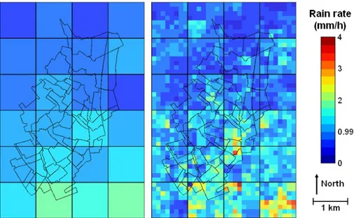
An example of the downscaled field for an arbitrary time step over the studied area of Cranbrook is presented in fig. 5. The same colour palette is used for both the radar and the downscaled field so that they can be compared. The effect of the downscaling that creates greater or smaller rainfall rate inside a given radar pixel is visible, especially in the south.
Figure 5: Illustration of the downscaling of the rainfall field over the Cranbrook area for an arbitrary time step of the February event and a 2D downscaling.
2.3.2) Comparison of the downscaling techniques
Before continuing, the 4 types of downscaling techniques tested should be compared. This involves comparing the fields obtained after 3 steps of spatial cascades (a map of 8 * 8 pixels) and 2 steps of spatio-temporal cascades (4 consecutive maps of 9 * 9 pixels), generated with the help of the same UM parameters. The results are discussed for the parameters of the February event, but similar conclusions are found as with the July event. To achieve the comparison 10 000 samples of 2D and 3D sub-cascades are generated, and the mean and maximum values are retrieved.
The probability distributions of the mean values are rather symmetric and the fluctuations around the average over all the samples are equal to 0.25 and 0.13 for respectively the 2D and the 3D non-normalised cascade schemes. The fluctuations around the average are not negligible, and are lost when normalising the fields. However, it should be mentioned that when a not-normalized cascade scheme is implemented, the total rainfall depth over the whole Cranbrook area (=19.14 mm for the February event) estimated with the radar is retrieved since numerous (256 time steps * 42 radar pixels) sub-cascades are generated,. Indeed, averaging over the 100 samples of downscaled field we find 19.14±0.07 mm and 19.14±0.04 mm respectively for the not-normalized 2D and 3D downscaling techniques. This means that the hydrological consequences observed when using the not-normalized field are due to a change in the spatial distribution of rainfall and not to a change of total rainfall amount.
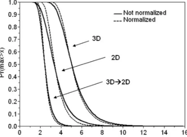
The excess distribution functions of the maximum values for the four cascade schemes are displayed in figure 6. The first conclusion is that, as expected (the ratio between the initial and the final resolution is greater in space and time for the 3D than for the 2D scheme; 9 to 8 in space and 4 to 1 in time) greater values are generated with the 3D scheme, in terms of mm/h over a pixel during a period of time. Nevertheless to actually compare the two schemes in terms of potential hydrological consequences, it seems more relevant to compare the 2D and 3D scheme at the same temporal resolution (the final spatial resolution are similar for both schemes). Therefore we considered the total amount of rain per pixels of the 3D scheme (i.e. the sum of the contribution of the 4 time steps over each pixel). The curve is denoted
3D2D and plotted fig. 6. In that case the maximum values generated are smaller than for the 2D scheme. Given that rainfall is a space-time process, it means that implementing the simpler 2D scheme might lead to extreme values greater than the one obtain with the more realistic 3D scheme. This is due to the fact that even if the extremes are greater for the 3D scheme, they remain valid during only 1.25 min whereas the one in the 2D scheme remain valid during 5 min. In the 3D case the extreme values are indeed not generated over the same spatial pixel. Concerning the differences between the normalized and not normalized field the distributions are quite similar. Nevertheless it can be noted that, for normalized fields this distribution is slightly more concentrated (smaller maximum values and greater minimum values).
Figure 6: Excess distribution function of the maximum value of the field obtained after 2 steps of spatio-temporal cascade and 3 steps of spatial cascade with the UM parameters of the February event.
3) Presentation of the rainfall - runoff model and case study
The case-study area chosen to perform the tests is the Cranbrook catchment in the London Borough of Redbridge. The Cranbrook catchment is a tributary of the Roding River that starts at Molehill Green and discharges into the Thames at Barking Creek. The Cranbrook catchment has a drainage area of approximately 900 ha. It is approximately 5.75 km long, of which 5.69 km is culverted. The catchment is predominantly urban with several parks (it has two lakes) and playing fields. This area has a history of local flooding. The computational rainfall/runoff model used was provided and calibrated by Thames Water Utilities Ltd (2002) and includes the major surface water sewers and associated ancillaries that drain to the River Roding. The area is divided into 51 sub-catchments (with areas ranging from 1 to 62 ha) that are considered homogeneous. The simulations were carried out using the Infoworks CS urban drainage simulation software (Wallingford Software, 2009). The simulation parameters were maintained unchanged for all simulations.
The version of Infoworks CS used here does not accept radar data as rainfall input. Therefore rainfall variability was taken into account by inputting a different time series for each sub-catchment. The average square root of the sub-catchment areas is 380 m, which is greater than the downscaled rainfall resolution of 125 m or 111 m (according to the technique used). This means that some information is lost in the process. Further investigations with a finer rainfall-runoff model and involving a better representation of surface flow (Maksimovic et al., 2009; Schmitt et al., 2004), should be performed to fully take advantage of the rainfall downscaling. In order to evaluate the rainfall time series corresponding to a sub-catchment,
the area of intersection between the sub-catchment and each downscaled pixel (Aij) was
estimated with the help of a GIS. Then for each time step the rainfall rate (R) is estimated as the weighted sum:
j i ij j i ij ijR A A R , , / (4)where Rij is the rainfall rate of the downscaled pixels. The total rainfall depth during the
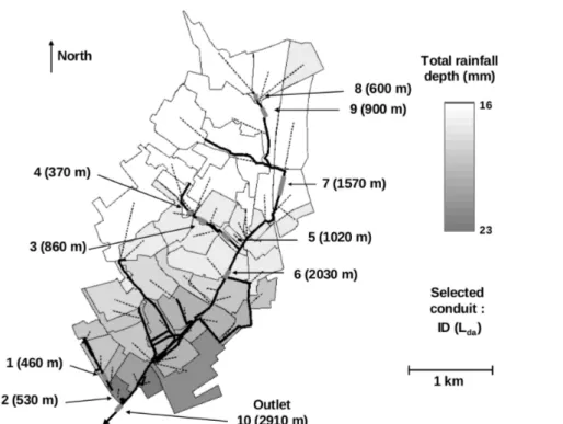
February event for each sub-catchment is displayed in fig. 7. It ranges from 16 to 23 mm. The rainfall distribution exhibits a similar spatial pattern for the July event, but with greater variation between the sub-catchments (from 4 to 14 mm).
The study is done by analysing the hydrographs of ten conduits. They were selected so that they cover a wide range of characteristic lengths (Lda), defined as the square root of the
area drained by the conduit. Lda is small for upstream pipes and larger for downstream pipes.
The relevance of this parameter will appear in section 4. The characteristic lengths of the selected conduits (see fig. 7) range from 370 to 2910 m.
Figure 7: The Cranbrook study case. Total rainfall depth during the February event for the 51 sub-catchments. The black lines represent the modelled underground sewer system.
4) Results and discussion
4.1) Impact of measured rainfall variability
In this section, the hydrographs obtained by using the radar distributed rainfall data (with the index ‘radar’) or the average rainfall over the whole Cranbrook catchment (index ‘avg’) are compared. We focused on the peak flow (PF) and evaluated the relative error:
radar radar avg PF PF PF error Relative (5)
for each selected conduit. Fig. 8 displays the results as a function of the characteristic length of the conduits. It ranges from -30 to +21% for the February event and from -65 to +349% for the July one. These values are large and certainly cannot be neglected, which means that there is a need to generalize the use of radar (see Einfalt et al., 2004, for a roadmap), or dense rain gauge networks, in order to properly simulate and possibly manage flows in sewer systems more efficiently. The relative error is negative for conduits 1, 2 and 10 (the outlet), positive for the others. This is not surprising since the heaviest rainfalls were located in the South during this event, which means that considering the average rainfall corresponds to virtual transfer of water from the South to the North. The absolute value of the relative error has a general tendency (clearer for the February event) to decrease with Lda, which is not surprising
since greater drained areas generally tend to damp the effect of rainfall variability. A deeper analysis of this dependency is performed in section 4.2.2. For the July event the outlet is very sensitive to the rainfall resolution and the damping effect that should be observed is not present because the nearest sub-catchments receive the heaviest rainfall. Finally it should be noted that some differences in terms of total volume are observed. They are due to the fact that the coefficients of imperviousness are not the same for all the sub-catchments (generally smaller in the northern part of the Cranbrook area).
Figure 8: Relative error of PFavg with regards to PFradar as a function of the characteristic
length (Lda) of the conduit.
4.2) Impact of small scale unmeasured rainfall variability
In the previous section, it was found that the error made by considering the average rain over the whole Cranbrook area rather than the radar distributed rainfall could not be neglected. It is expected that the same kind of error will occur between the 1 km radar resolution rainfall and higher resolutions. Unfortunately no rainfall data are available to directly confirm that statement. To overcome this difficulty the field is stochastically downscaled. For each type of downscaling technique, an ensemble of 100 samples was generated. The statistical analysis of the corresponding ensemble of simulated hydrographs enables the quantification of the potential uncertainty due to the unknown small scale rainfall variability.
4.2.1) Analysis of the peak flow
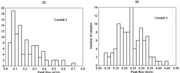
Before analysing the whole hydrograph, we first focus on the peak flow, which is of prime interest in the management of sewer systems. For each sample the peak flow and its occurrence time was estimated. Histograms of the peak flow distribution among the 100 samples with the 2D and 3D downscaling technique are displayed in fig. 9 for conduit 2 and the February events. The patterns of these histograms are representative of the other conduits and event. In order to quantify the variability among the samples, the classical coefficient of variation (i.e. the ratio between the standard deviation and the mean) is typically used. However in that specific case, it is more relevant to define a coefficient of variation CV’ with the help of the 10 and 90 % quantiles (denoted respectively PF0.1 and PF0.9) to take into
account the non gaussianity, in particular the skewness, of the histograms (more pronounced for the spatial than for the spatio-temporal downscaling). CV’ is defined as follows:
radar PF PF PF CV * 2 ' 0.9 0.1 (6)
CV’ quantifies the uncertainty associated to the unknown high resolution rainfall variability. The use of percentages allows for comparison of the results for all the conduits despite the differences in the values of the peak flow.
Figure 9: Histograms of the peak flow of the 100 samples for conduit 2, the February event and the 2D and 2D downscaling.
Fig. 10 shows CV’ vs. Lda for the 4 types of downscaling and both events. The order of
magnitude of CV’ is comparable to the relative error between averaged and radar rainfall (fig. 8), which was expected. Concerning the differences between the downscaling techniques, mainly two points should be highlighted. First, when the field is normalized so that it equals the measured radar rainfall at the observed resolution of 1 km (either in 2D or 3D), the uncertainty is slightly smaller than when it is not. This is expected since the normalization smoothes a little the natural behaviour of the cascade. Second, the uncertainty is greater for the spatial downscaling (2D and 2D_n) than for the spatio-temporal one (3D and 3D_n). This reflects the fact that in the more realistic spatio-temporal downscaling the variability (at similar scale) generated is smaller than in the spatial one (as previously mentioned in section 2.3.2). It means that the greater uncertainty exhibited when implementing the spatial downscaling is likely to be an overestimation. For the February event, CV’ clearly decreases with Lda, which is quite natural since a greater drained area will smooth the effect of small
scale variability. A power law fit to this decrease will be investigated in the next section. This tendency is also observed for the July event, but less clearly, especially for the outlet. This is
likely to be due to the fact that the heaviest rainfalls are very localized and near the outlet, which makes it very reactive. It is interesting to note that despite the coarse resolution of the rainfall-runoff model (the average square root of the sub-catchment area is 380 m) with regards to the downscaled rainfall resolution (125 m or 111 m), the uncertainty due to the unknown small scale rainfall variability cannot be neglected. It suggests that this type of ensemble prediction approach should be implemented in real time monitoring of sewer systems.
Finally, it should be mentioned that the effect on the timing of the peak flow is very limited. Since the order of magnitude of the variability was about few minutes, it was not investigated further.
Figure 10: CV’ as a function of the characteristic length Lda for both events.
4.2.2) Analysis of the hydrographs
In this section a similar approach was developed, not only for the peak flow, but also for the whole hydrograph. Twenty hydrographs, centred on the peak flow, arbitrarily selected among the 100 generated are plotted on fig. 11 for conduit 2, for both events under the 3D downscaling scheme. The variability inside the ensemble of simulated hydrographs is visible. In order to clarify these curves, for each time step the 10, 50 (median) and 90% quantiles were estimated, which enables the generation of the corresponding temporal evolution of the flow (respectively Q0.9(t), Q0.5(t), Q0.1(t)). Fig. 11 displays these curves and Qradar for conduit 2,
both events and the 3D downscaling. Similar curves are obtained for other conduits and types of downscaling. For the February event, it can be seen that the uncertainty observed for the peak flow is also observed for each smaller peak. The median (Q0.5) is also very close to Qradar
(the curves almost cannot be distinguished). For the July event the situation is more complex. First of all, Q0.5 is not always similar to Qradar. This is probably due to the fact that the
histograms of the distribution for each time step are more skewed than for the February event. Moreover Q0.1 and Q0.9 are quite different which means that the range of realistic scenarios
covered with the rainfall downscaling is wide, and that there is a huge uncertainty on the actual flow (the one with a perfectly known rainfall). This result suggests that for this type of convective event, the observed resolution of 1 km is not fine enough.
Figure 11: Twenty samples of the ensemble of hydrographs simulated with a 3D downscaling for conduit 2, February (a) and July events (b). Hydrographs Q0.9 (dash), Q0.5 (dash dot), Q0.1
(dash) and Qradar for conduit 2 and February (c) and July (d) events.
Real time management of sewer systems, including forecasting, could benefit from taking into account the uncertainty associated with the unknown small scale rainfall variability. These applications require short computational time, which is especially critical in times of flooding. Indeed, one of the critical aspects of flood forecast for emergency management purposes is the period of time available between the acquisition of data, such as rainfall, and the results obtained by hydraulic simulations. Therefore, data transmission, rainfall forecast and hydraulic simulation of the drainage system need to be fast, reliable and as accurate as possible in order to get the best possible estimation of inundation extent, depth and peak time with sufficient time to permit successful operational responses (Simões et al, 2010). It is not at the moment possible to generate 100 samples and simulate the corresponding hydrographs in the sewer system in the available time (it takes roughly one hour on a standard laptop). In order to avoid doing these simulations in real time (where computational time is critical), in the following,Q0.9 is investigated as a function of Qradar,
with the aim of determining a standard relation between these variables, which could be directly used for assessing the uncertainty associated with the unknown small scale rainfall variability.
The first step is to look at Q0.9 vs. Qradar in a log-log plot. Fig. 12 shows this plot for
conduit 2 during the February event and for a 3D downscaling. It should be mentioned that only the time steps when Qradar(t)>PFradar/10 are considered, to avoid taking into account small
flow values which are not relevant here. Similar plots are found for other conduits and types of downscaling. The graphs seem to exhibit a linear pattern, which means that Q0.9 and Qradar
are linked by a power law of coefficients a and b defined as follows:
a radar
bQ
Q0.9 (7)
For the February event, the coefficient of determination of these linear regressions is equal to 0.99±0.01 on average (depending on the conduits and the type of downscaling) which means
that the power law relation is appropriate. For the July event this average is equal to 0.95±0.06, which remains good. On some of the log-log plots it should be mentioned that some “loops” appear (slightly visible in fig. 12). They correspond to the increasing or decreasing portion of the same peak, which do not exhibit the same behaviour (the differences between Q0.9 and Qradar are greater for a decreasing flow). The linear regression does not
allow us to model this effect, but rather provides an average measure of the uncertainty.
Figure 12: Log-log plot of Q0.9 vs. Qradar for conduit 2 and the 3D downscaling of the
February event. The coefficient of determination of the linear regression is 0.99, and a and b
are respectively equal to 1.01 and 1.21
The values of exponent a are displayed as a function of Lda in fig. 13. The 95%
confidence intervals are greater for the July event because the coefficients of determination are smaller, and also because fewer points are considered in the linear regression (the peak flow lasts roughly 1 h whereas it lasts 5 h for the February event). The first striking feature is that they basically do not significantly depend on the type of downscaling used. There is also no clear evidence of any dependence on Lda. The average value of a is roughly 1.0 for the
February event and 1.1 for the July one. These values are quite comparable despite the differences in the nature of the events. Note that a is very close to 1, i.e. Q0.9 is almost
linearly related to Qradar. It is likely to be due to the fact that, as already mentioned, the spatial
resolution of the model does not enable one to fully take into account the generated rainfall variability. Similar behaviour is observed on Q0.1.
Figure 13: a vs. Lda for both events. The vertical bars correspond to the confidence interval for
As for the values of b, they are displayed on fig. 14 as a function of Lda in a log-log
plot. The graphs seem to exhibit a linear behaviour which means b would be related to Lda by
a power law of coefficients c and d, defined as follow:
c da
dL
b (8)
For both events, conduits 8 and 9, which are located in the North of the catchment where the rain rates are much lower than elsewhere, are not taken into account in the linear regression because they would significantly worsen it. For the February event the coefficients of determination of the linear regression range from 0.85 to 0.91, which means the power law relation is relevant. It means that Q0.9 exhibits a scaling behaviour with regards to the spatial
resolution (“represented” here by Lda). For the July event the coefficients of determination are
lower (from 0.26 to 0.80) which implies that the 95 % confidence intervals for the intercept and the slope are broad and the values are less accurate for that event. This could be explained by the fact that, as previously mentioned, the outlet is very reactive, and moreover that the radar rainfall resolution of 1 km does not seem to be high enough. Fig. 15.a and 15.b display the values found for respectively c and d. Given the size of the 95 % confidence intervals it is hard to conclude as to the dependency of c and d with regard to the events and the type of downscaling. Nevertheless it appears that the values of c for the July event are slightly greater than for the February event. This indicates a quicker decrease of Q0.9 with larger areas, which
reflects the local nature of convective event. Concerning d, it seems that it is slightly greater for the July event than for the February one, indicating greater uncertainty for convective than for frontal events. d seems be smaller with the spatio-temporal than for the spatial downscaling reflecting smaller (but certainly more realistic) uncertainty.
As a conclusion to this section, it appears that Q0.9which quantifies the uncertainty
due to the unknown small scale rainfall variability follows the double power law relation:
a radar c da Q dL Q0.9 (9)
where a (11.1) depends neither on the type of downscaling nor the event, which means it is quite robust (given the spatial resolution of the model compared to that of the rainfall). On the other hand, c and d depend on the type of downscaling and/or the event, and should therefore be calibrated using the observed rainfall data. Further investigations are required to understand how to calibrate them.
Figure 14: b vs. Lda in a log-log plot for both events. The vertical bars correspond to the
confidence interval for the 2D downscaling. They are representative of the other types of downscaling. Conduit 8 and 9 (pointed in the graphs) are not taken into account in the linear regression.
Figure 15: c (a) and d (b) with 95% confidence interval for both events and the four downscaling techniques.
5) Conclusion
The aim of this paper was to analyse the impact of rainfall variability on the hydrographs of sewer conduits simulated by a semi-distributed urban rainfall-runoff model. The study was performed on the 900 ha urban catchment of Cranbrook in the east of London (United-Kingdom). Two rainfall events were analysed: a convective summer one and a frontal winter one.
The first step of the study consists in comparing the hydrographs obtained by using the radar distributed rainfall field and the average rain over the whole catchment. The relative error produced on the peak flow by using the average rain rather than the radar one is significant. Indeed it ranges from -30 to 21 % for the February event and from -65 to 349 % for the July event.
A kind of ensemble prediction approach was then implemented to quantify the uncertainty due to the unmeasured small scale variability, i.e below the radar resolution. An analysis of the quantiles of the simulated peak flows showed that the uncertainty for the outlet was equal to 3% for the February event and 20% for the July event, and reached respectively 25 % and 40 % for some conduits, with the spatio-temporal downscaling. The uncertainty found with the spatial downscaling is greater but reflects the fact that the spatial downscaling tends to generate stronger rainfall extremes than the more realistic spatio-temporal downscaling. The same features are retrieved on the whole hydrograph. An ensemble prediction approach is too time-consuming to be implemented in real time management of sewer systems. As a consequence, a quick way of estimating the flow corresponding to the 90 % quantile was developed. It was found that the latter, the flow simulated with the radar rainfall and the characteristic length of the sewer conduit (i.e. the square root of the area it drains) are related by a double power law. These results should be confirmed by other studies with a direct modelling of surface flow and a finer resolution of the rainfall-runoff model.
The results of this study show that it is strongly recommended to use radar distributed rainfall in urban hydrology. The use of X-band radar which allows measuring rainfall at a higher resolution than the standard available one of 1 km should also be generalized. This is especially true for convective events for which the limitations of 1 km resolution are clearly exhibited in this study. Moreover, the uncertainty due to the unknown small scale rainfall variability certainly cannot be neglected and should therefore be taken into account in a probabilistic way in the real time management of sewer systems.
A. Gires highly acknowledges the Université Paris-Est, the Chair “Hydrology for Resilient Cities” (sponsored by Veolia) of Ecole des Ponts ParisTech and the EU FP7 SMARTesT project for their financial supports that made possible his visit to Imperial College. A. Gires also acknowledges the EWRE section of Imperial College London, Department of Civil and Environmental Engineering for partial financial support. The research was conducted as part of the Flood Risk Management Research Consortium (FRMRC2, SWP3). The authors would also like to thank the UK Met Office and the universities of Swansea and Bristol for providing the Nimrod data for the study area with which the analysis presented in this article was performed. The authors would like to acknowledge MWH Soft the provision of the software, and Thames Water Utilities Ltd for the runoff model data. N. Simões acknowledges the financial support from the Fundação para a Ciência e Tecnologia - Ministério para a Ciência, Tecnologia e Ensino Superior, Portugal [SFRH/BD/37797/2007].
References
Arnaud, P., Bouvier, C., Cisneros, L., Dominguez, R., 2002. Influence of rainfall spatial variability on flood prediction. J. Hydrol. 260, 216-230.
Aronica, G., Cannarozzo, M., 2000. Studying the hydrological response of urban catchments using a semi-distributed linear non-linear model. J. Hydrol. 238, 35-43.
Biaou, A., Hubert, P., Schertzer, D., Tchiguirinskaia, I., Bendjoudi, H., 2003. Fractals, multifractals et prévision des précipitations. Sud Sciences et Technologies 10, 10-15.
Chambers, J.M., Mallows, C.L., Stuck, B.W., 1976. A method for simulating stable random variables. Journal of the American statistical Association 71, 340-344.
Deidda, R., 2000. Rainfall downscaling in a space-time multifractal framework. Water Resour. Res. 36, 1779-1794.
de Lima, J.L.M.P., Singh V.P., 2002. The influence of moving rainstorms on overland flow, Adv. Water Resour. 25, 817-828.
de Lima, M.I.P., Grasman, J., 1999. Multifractal analysis of 15-min and daily rainfall from a semi-arid region in Portugal. J. Hydrol. 220, 1-11
de Montera, L., Barthes, L., Mallet, C., Gole, P., 2009. The Effect of Rain-No Rain Intermittency on the Estimation of the Universal Multifractals Model Parameters. J. Hydromet. 10(2), 493-506.
Desaulnier-Soucy, N., Lovejoy, S., Schertzer, D., 2001. The continuum limit in rain and the HYDROP experiment. J. Atm. Res. 59-60, 163-197.
Dodov, B., Foufoula-Georgiou, E., 2005. Incorporating the spatio-temporal distribution of rainfall and basin geomorphology into nonlinear analyses of streamflow dynamics. Adv. Water Resour. 28, 711-728.
Einfalt, T., Arnbjerg-Nielsen, K., Golz, C., Jensen, N.-E., Quirmbach, M., Vaes, G., Vieux, B., 2004. Towards a roadmap for use of radar rainfall data in urban drainage. J. Hydrol. 299, 186– 202.
Faurès, J.-M., Goodrich, D.C., Woolhiser, D.A., Sorooshian, S., 1995. Impact of small-scale spatial rainfall variability on runoff modelling. J. Hydrol. 173, 309-326.
Ferraris, L., Gabellani, S., Rebora, N., Provenzale, A., 2003. A comparison of stochastic models for spatial rainfall downscaling. Water Resour. Res. 39, 1368–1384.
Gires, A., Tchiguirinskaia, I., Schertzer, D., Lovejoy, S., 2010. Influence of the zero-rainfall in the multifractal estimates of the extremes. Submitted to Adv. Water Resour.
Gires, A., Tchiguirinskaia, I., Schertzer, D., Lovejoy, S., 2011. Analyses multifractales et spatio-temporelles des précipitations du modèle Méso-NH et des données radar. Hydrol. Sci. J. 56(3), 380-396.
Gupta, V.K., Waymire, E., 1993. A Statistical Analysis of Mesoscale Rainfall as a Random Cascade. J. Appl. Meteor. 32, 251-267.
Harris, D., Menabde, M., Seed, A., Austin, G., 1997. Factors affecting multiscaling analysis of rainfall time series. Nonlin. Processes Geophys. 4, 137-155.
Harrison, D.L., Driscoll, S.J., Kitchen, M., 2000. Improving precipitation estimates from weather radar using quality control and correction techniques. Met. Appl. 7(2), 135–144.
Kolmogorov, A.N., 1962. A refinement of previous hypotheses concerning the local structure of turbulence in viscous incompressible fluid at high Reynolds number. J. Fluid. Mech. 13, 82-85.
Lavallée, D., Lovejoy, S., Ladoy, P., 1993. Nonlinear variability and landscape topography: analysis and simulation, in: De Cola, L., Lam, N. (Eds.), Fractals in geography. Prentice-Hall, New-York., pp. 171-205.
Lhomme, J., Bouvier, C., Perrin, J.-L., 2004. Applying a GIS-based geomorphological routing model in urban catchments. J. Hydrol. 299, 203–216.
Lovejoy, S., Schertzer, D., 2007. Scaling and multifractal fields in the solid earth and topography. Nonlin. Processes Geophys. 14, 465-502.
Lovejoy, S., Schertzer, D., 2010. On the simulation of continuous in scale universal multifractals, part I: spatially continuous processes, in press Computers and Geoscience.
Macor, J., Schertzer, D., Lovejoy, S., 2007. Multifractal Methods Applied to Rain Forecast Using Radar Data. La Houille Blanche 4, 92-98.
Maksimović, Č., Prodanović, D., Boonya-aroonnet, S., Leitão, J. P., Djordjević, S., Allitt, R., 2009. Overland flow and pathway analysis for modelling of urban pluvial flooding. Journal of Hydraulic Research 47(4), 512–523.
Mandapaka, P.V., Lewandowski, P., Eichinger, W.E., Krajewski, W.F., 2009. Multiscaling analysis of high resolution space-time lidar-rainfall. Nonlin. Processes Geophys. 16, 579–586.
Marsan, D., Schertzer, D., Lovejoy, S., 1996. Causal space-time multifractal processes: Predictability and forecasting of rain fields. J. Geophys. Res. 101(26), 333-326.
Menabde, M., Harris, D., Seed, A., Austin, G., Stow, D., 1997. Multi-scaling properties of rainfall and bounded random cascades. Water Resour. Res. 33, 2823–2830.
Nykanen, D.K., 2008. Linkages between Orographic Forcing and the Scaling Properties of Convective Rainfall in Mountainous Regions. J. Hydromet. 9, 327-347.
Nykanen, D.K., Harris, D., 2003. Orographic influences on the multiscale statistical properties of precipitation. J. Geophys. Res., 108(D8), 8381-8993.
Olsson, J., Niemczynowicz, J., 1996. Multifractal analysis of daily spatial rainfall distributions. J. Hydrol. 187, 29-43.
Olsson, J., Uvo, C.B., Jinno, K., 2001. Statistical atmospheric downscaling of short-term extreme rainfall by neural networks. Phys. Chem. Earth (B) 26(9), 695-700.
Over, T.M., Gupta, V.K., 1996. A space-time theory of mesoscale rainfall using random cascades. J. Geophys. Res. 101(D21), 26319-26331.
Parisi, G., Frish, U.,1985. A multifractal model of intermittency, in: Ghill, M., Benzi, R., and Parisi, G. (Eds), Turbulence and predictability in geophysical fluid dynamics. North Holland. p. 111-114.
Pecknold, S., Lovejoy, S., Schertzer, D., Hooge, C., Malouin, J.F., 1993. The simulation of universal multifractals, in: Perdang, J.M., Lejeune A. (Eds), Cellular Automata: Prospects in astrophysical applications. World Scientific, pp 228-267.
Radkevich, A., Lovejoy, S., Strawbridge, K., Schertzer, D., Lilley, M., 2008. Scaling turbulent atmospheric stratification, Part III: Space-time stratification of passive scalars from lidar data. Quart. J. Roy. Meteor. Soc. 134, 316-335.
Rebora, N., Ferraris, L., von Hardenberg, J., Provenzale, A., 2006a. The RainFARM: Downscaling LAM predictions by a Filtered AutoRegressive Model. J. Hydromet. 7, 724-737.
Rebora, N., Ferraris, L., von Hardenberg, J., Provenzale, A., 2006b. Rainfall downscaling and flood forecasting: a case study in the Mediterranean area. Nat. Hazards Earth Syst. Sci. 6, 611–619.
Royer, J.F., Biaou, A., Chauvin, F., Schertzer, D., Lovejoy, S., 2008. Multifractal analysis of the evolution of simulated precipitation over France in a climate scenario. C.R Geoscience 340, 431-440.
Schertzer, D., Lovejoy, S., 1987a. Physical modelling and analysis of rain and clouds by anisotropic scaling and multiplicative processes. J. Geophys. Res. 92(D8), 9693-9714.
Schertzer, D., Lovejoy, S., 1987b. Singularités anisotropes, divergences des moments en turbulence: invariance d’échelle généralisée et processus multiplicatifs. Ann. Sci. Math. Que. 11(1), 139-181.
Schertzer, D., Lovejoy, S., 1989. Nonlinear variability in geophysics multifractal analysis and simulations, in: Pietronero, L. (Ed), Fractals Physical Origin and properties. Plenum Press: New-York., pp. 41-82.
Schertzer, D., Lovejoy, S., Schmitt, F., Tchiguirinskaia, I., Marsan, D., 1997. Multifractal cascade dynamics and turbulent intermittency. Fractals 5(3), 427-471.
Schertzer, D., Lovejoy, S., Hubert, P, 2002. An introduction to stochastic multifractal fields, in: Ern, A. and Liu, W. (Eds), Isfma symposium on environmental science and engineering with related mathematical problems. High Education Press: Beijing, pp. 106-179.
Schertzer, D., Tchiguirinskaia, I., Lovejoy, S., Hubert, P., 2010. No monsters, no miracles: in nonlinear sciences hydrology is not an outlier!. Hydrol. Sci. J. 55(6), 965-979.
Schertzer, D., Loveloy, S., 2011. Multifractals, generalized scale invariance and complexity in geophysics. International Journal of Bifurcation and Chaos 21(12), 3417–3456.
Schmitt, F., Vannitsem, S., Barbosa, A., 1998. Modeling of rainfall time series using two-state renewal processes and multifractals. J. Geophys. Res. 103(D18), 23181-23193.
Schmitt, T.G., Thomas, M., Ettrich, N., 2004. Analysis and modeling of flooding in urban drainage systems. J. Hydrol. 298, 300–311.
Segond, M.L., Wheater, H.S., Onof, C., 2007. The significance of small-scale spatial rainfall variability on runoff modelin. J. Hydrol. 173, 309-326.
Simões, N.E., Leitão, J.P., Maksimović, Č., Sá Marques, A., Pina, R., 2010. Sensitivity Analysis of Surface Runoff Generation in Urban Floods Forecasting. Water Science & Technology 61(10), 2595–2601.
Singh, V.P., 1997. Effect of spatial and temporal variability in rainfall and watershed characteristics on stream flow hydrograph. Hydrol. Process. 11, 1649-1669.
Smith, M.B., Koren, V.I., Zhang, Z., Reeda, S.R., Panb J.J., Moredaa, F., 2004. Runoff response to spatial variability in precipitation: an analysis of observed data. J. Hydrol. 298, 267-286.
Tessier, Y., Lovejoy, S., Schertzer, D., 1993. Universal Multifractals: theory and observations for rain and clouds. J. Appl. Meteor. 32(2), 223-250.
Thames Water Utilities Ltd Engineering, 2002. Surface Water Model Of CranBrook And Seven Kings Water For London Borough Of Redbridge Appendix B, Model Development Report.
Verrier, S., de Montera, L., Barthes, L., Mallet, C., 2010. Multifractal analysis of African monsoon rain fields, taking into account the zero rain-rate problem. J. Hydrol. 389(1-2), 111-120.
Vieux, B.E., Bedient, P.B., 2004. Assessing urban hydrologic prediction accuracy through event reconstruction. J. Hydrol. 299, 217–236.