Using Stocks or Portfolios in
Tests of Factor Models
∗
Andrew Ang
†Columbia University and NBER
Jun Liu
‡UCSD
Krista Schwarz
§University of Pennsylvania
This Version: 7 September, 2010
JEL Classification: G12
Keywords: Specifying Base Assets, Cross-Sectional Regression,
Estimating Risk Premia, APT, Efficiency Loss
∗We thank Rob Grauer, Cam Harvey, Bob Kimmel, Georgios Skoulakis, Yuhang Xing, and Xiaoyan Zhang for helpful discussions and seminar participants at the American Finance Association, Columbia University, CRSP forum, Texas A&M University, and the Western Finance Association for comments. We thank Bob Hodrick, Raymond Kan, an anonymous associate editor, and two anonymous referees for detailed comments which greatly improved the paper.
†Columbia Business School, 3022 Broadway 413 Uris, New York, NY 10027, ph: (212) 854-9154; email: [email protected]; WWW: http://www.columbia.edu/∼aa610.
‡Rady School of Management, Otterson Hall, 4S148, 9500 Gilman Dr, #0553, La Jolla, CA 92093-0553; ph: (858) 534-2022; email: [email protected]; WWW: http://rady.ucsd.edu/faculty/directory/liu/.
§The Wharton School, University of Pennsylvania, 3620 Locust Walk, SH-DH 2300, Philadelphia, PA 19104; email: [email protected]
Using Stocks or Portfolios in
Tests of Factor Models
Abstract
We examine the efficiency of using individual stocks or portfolios as base assets to test asset pricing models using cross-sectional data. The literature has argued that creating portfolios reduces idiosyncratic volatility and allows factor loadings, and consequently risk premia, to be estimated more precisely. We show analytically and demonstrate empirically that the smaller standard errors of beta estimates from creating portfolios do not lead to smaller standard errors of cross-sectional coefficient estimates. The standard errors of factor risk premia estimates are determined by the cross-sectional distributions of factor loadings and residual risk. Creating portfolios destroys information by shrinking the dispersion of betas and leads to larger standard errors.
1
Introduction
Asset pricing models should hold for all assets, whether these assets are individual stocks or whether the assets are portfolios. The literature has taken two different approaches in specifying the universe of base assets in cross-sectional factor tests. First, researchers have followed Black, Jensen and Scholes (1972) and Fama and MacBeth (1973), among many others, to group stocks into portfolios and then run cross-sectional regressions using portfolios as base assets. An alternative approach is to estimate cross-sectional risk premia using the entire universe of stocks following Litzenberger and Ramaswamy (1979) and others. Perhaps due to the easy availability of portfolios constructed by Fama and French (1993) and others, the first method of using portfolios as test assets is the more popular approach in recent empirical work.
Blume (1970, p156) gave the original motivation for creating test portfolios of assets as a way to reduce the errors-in-variables problem of estimated betas as regressors:
...If an investor’s assessments of αi andβi were unbiased and the errors in these
assessments were independent among the different assets, his uncertainty attached to his assessments ofα¯andβ¯, merely weighted averages of theαi’s andβi’s, would
tend to become smaller, the larger the number of assets in the portfolios and the smaller the proportion in each asset. Intuitively, the errors in the assessments ofαi
andβi would tend to offset each other. ... Thus, ...the empirical sections will only
examine portfolios of twenty or more assets with an equal proportion invested in each.
If the errors in the estimated betas are imperfectly correlated across assets, then the estimation errors would tend to offset each other when the assets are grouped into portfolios. Creating portfolios allows for more efficient estimates of factor loadings. Blume argues that since betas are placed on the right-hand side in cross-sectional regressions, the more precise estimates of factor loadings for portfolios enable factor risk premia to also be estimated more precisely. This intuition for using portfolios as base assets in cross-sectional tests is echoed by other papers in the early literature, including Black, Jensen and Scholes (1973) and Fama and MacBeth (1973). The majority of modern asset pricing papers testing expected return relations in the cross section now use portfolios.1
1Fama and French (1992) use individual stocks but assign the stock beta to be a portfolio beta, claiming to be able to use the more efficient portfolio betas but simultaneously using all stocks. We show below that this procedure is equivalent to directly using portfolios.
In this paper we study the relative efficiency of using individual stocks or portfolios in tests of cross-sectional factor models. We focus on theoretical results in a one-factor setting, but also consider multifactor models and models with characteristics as well as factor loadings. We illustrate the intuition with analytical forms using maximum likelihood, but the intuition from these formulae are applicable to more general situations.2 Maximum likelihood estimators
achieve the Cram´er-Rao lower bound and provide an optimal benchmark to measure efficiency. The Cram´er-Rao lower bound can be computed with any set of consistent estimators.
Forming portfolios dramatically reduces the standard errors of factor loadings due to de-creasing idiosyncratic risk. But, we show the more precise estimates of factor loadings do not lead to more efficient estimates of factor risk premia. In a setting where all stocks have the same idiosyncratic risk, the idiosyncratic variances of portfolios decline linearly with the num-ber of stocks in each portfolio. But, the standard errors of the risk premia estimates increase when portfolios are used compared to the case when all stocks are used. The same result holds in richer settings where idiosyncratic volatilities differ across stocks, idiosyncratic shocks are cross-sectionally correlated, and there is stochastic entry and exit of firms in unbalanced pan-els. Thus, creating portfolios to reduce estimation error in the factor loadings does not lead to smaller estimation errors of the factor risk premia.
The reason that creating portfolios leads to larger standard errors of cross-sectional risk premia estimates is that creating portfolios destroys information. A major determinant of the standard errors of estimated risk premia is the cross-sectional distribution of risk factor load-ings scaled by the inverse of idiosyncratic variance. Intuitively, the more disperse the cross section of betas, the more information the cross section contains to estimate risk premia. More weight is given to stocks with lower idiosyncratic volatility as these observations are less noisy. Aggregating stocks into portfolios shrinks the cross-sectional dispersion of betas. This causes estimates of factor risk premia to be less efficient when portfolios are created. We compute efficiency losses under several different assumptions, including cross-correlated idiosyncratic risk and betas, and the entry and exit of firms. The efficiency losses are large.
Finally, we empirically verify that using portfolios leads to wider standard error bounds in estimates of one-factor and three-factor models using the CRSP database of stock returns. We find that for both a one-factor market model and the Fama and French (1993) multifactor model estimated using the full universe of stocks, the market risk premium estimate is positive
2Jobson and Korkie (1982), Huberman and Kandel (1987), MacKinlay (1987), Zhou (1991), Velu and Zhou (1999), among others, derive small-sample or exact finite sample distributions of various maximum likelihood statistics but do not consider efficiency using different test assets.
and highly significant. In contrast, using portfolios often produces insignificant and sometimes negative point estimates of the market risk premium in both one- and three-factor specifications. We stress that our results do not mean that portfolios should never be used to test factor models. In particular, many non-linear procedures can only be estimated using a small num-ber of test assets. However, when firm-level regressions specify factor loadings as right-hand side variables, which are estimated in first stage regressions, creating portfolios for use in a second stage cross-sectional regression leads to less efficient estimates of risk premia. Second, our analysis is from an econometric, rather than from an investments, perspective. Finding investable strategies entails the construction of optimal portfolios. Finally, our setting also con-siders only efficiency and we do not examine power. A large literature discusses how to test for factors in the presence of spurious sources of risk (see, for example, Kan and Zhang, 1999; Kan and Robotti, 2006; Hou and Kimmel, 2006; Burnside, 2007) holding the number of test assets fixed. From our results, efficiency under a correct null will increase in all these settings when individual stocks are used. Other authors like Zhou (1991) and Shanken and Zhou (2007) examine the small-sample performance of various estimation approaches under both the null and alternative.3 These studies do not discuss the relative efficiency of the test assets employed
in cross-sectional factor model tests.
Our paper is related to Kan (2004), who compares the explanatory power of asset pric-ing models uspric-ing stocks or portfolios. He defines explanatory power to be the squared cross-sectional correlation coefficient between the expected return and its counterpart specified by the model. Kan finds that the explanatory power can increase or decrease with the number of portfolios. From the viewpoint of Kan’s definition of explanatory power, it is not obvious that asset pricing tests should favor using individual stocks. Unlike Kan, we consider the criterion of statistical efficiency in a standard cross-sectional linear regression setup. In contrast, Kan’s explanatory power is not directly applicable to standard econometric settings. We also show that using portfolios versus individual stocks matters in actual data.
Two other related papers which examine the effect of different portfolio groupings in testing asset pricing models are Berk (2000) and Grauer and Janmaat (2004). Berk addresses the issue of grouping stocks on a characteristic known to be correlated with expected returns and then
3Other authors have presented alternative estimation approaches to maximum likelihood or the two-pass methodology such as Brennan, Chordia and Subrahmanyam (1998), who run cross-sectional regressions on all stocks using risk-adjusted returns as dependent variables, rather than excess returns, with the risk adjustments involving estimated factor loadings and traded risk factors. This approach cannot be used to estimate factor risk premia.
testing an asset pricing model on the stocks within each group. Rather than considering just a subset of stocks or portfolios within a group as Berk examines, we compute efficiency losses with portfolios of different groupings using all stocks, which is the usual case done in practice. Grauer and Janmaat do not consider efficiency, but show that portfolio grouping under the alternative when a factor model is false may cause the model to appear correct.
The rest of this paper is organized as follows. Section 2 presents the econometric theory and derives standard errors concentrating on the one-factor model. We describe the data and com-pute efficiency losses using portfolios as opposed to individual stocks in Section 3. Section 4 compares the performance of portfolios versus stocks in the CRSP database. Finally, Section 5 concludes.
2
Econometric Setup
2.1
The Model and Hypothesis Tests
We work with the following one-factor model (and consider multifactor generalizations later):
Rit =α+βiλ+βiFt+σiεit, (1)
whereRit, i = 1, ..., N and t = 1, ..., T, is the excess (over the risk-free rate) return of stock
i at timet, andFt is the factor which has zero mean and variance σF2. We specify the shocks
εit to be IID N(0,1) over time t but allow cross-sectional correlation across stocks i and j.
We concentrate on the one-factor case as the intuition is easiest to see and present results for multiple factors in the Appendix. In the one-factor model, the risk premium of assetiis a linear function of stocki’s beta:
E(Rit) =α+βiλ. (2)
This is the beta representation estimated by Black, Jensen and Scholes (1972) and Fama and MacBeth (1973). In vector notation we can write equation (1) as
Rt =α1 +βλ+βFt+ Ω1/2ε εt, (3)
where Rt is a N ×1 vector of stock returns,α is a scalar, 1 is aN ×1vector of ones, β =
(β1 . . . βN)′ is anN ×1vector of betas,Ωε is anN ×N invertible covariance matrix, andεt
is anN ×1vector of idiosyncratic shocks whereεt∼N(0, IN).4
4The majority of cross-sectional studies do not employ adjustments for cross-sectional correlation, such as the recent paper by Fama and French (2008). We account for cross-sectional correlation in our empirical work in
Asset pricing theories impose various restrictions on α andλ in equations (1)-(3). Under the Ross (1976) Arbitrage Pricing Theory (APT),
H0α=0 : α= 0. (4)
This hypothesis implies that the zero-beta expected return should equal the risk-free rate. A rejection ofHα=0
0 means that the factor cannot explain the average level of stock returns. This
is often the case for factors based on consumption-based asset pricing models because of the Mehra-Prescott (1985) equity premium puzzle, where a very high implied risk aversion is nec-essary to match the overall equity premium.
However, even though a factor cannot price the overall market, it could still explain the relative prices of assets if it carries a non-zero price of risk. We say the factorFtis priced with
a risk premium if we can reject the hypothesis:
H0λ=0 : λ= 0. (5)
A simultaneous rejection of both H0α=0 and H0λ=0 economically implies that we cannot fully explain the overall level of returns (the rejection of Hα=0
0 ), but exposure to Ft accounts for
some of the expected returns of assets relative to each other (the rejection of Hλ=0
0 ). By far
the majority of studies investigating determinants of the cross section of stock returns try to rejectH0λ=0by finding factors where differences in factor exposures lead to large cross-sectional differences in stock returns. Recent examples of such factors include aggregate volatility risk (Ang et al., 2006), liquidity (P´astor and Stambaugh, 2003), labor income (Santos and Veronesi, 2006), aggregate investment, and innovations in other state variables based on consumption dynamics (Lettau and Ludvigson, 2001b), among many others. All these authors reject the null
Hλ=0
0 , but do not test whether the set of factors is complete by testingH0α=0.
In specific economic models such as the CAPM or if a factor is tradeable, then defining
˜
Ft=Ft+µ, whereF˜tis the non-zero mean factor withµ= E( ˜Ft), we can further test if
H0λ=µ : λ−µ= 0. (6)
This test is not usually done in the cross-sectional literature but can be done if the set of test assets includes the factor itself or a portfolio with a unit beta (see Lewellen, Nagel and Shanken, 2010). We show below, and provide details in the Appendix, that an efficient test for H0λ=µ is equivalent to the test forH0λ=0 and does not require the separate estimation of µ. If a factor is
priced (so we rejectHλ=0
0 ) and in addition we rejectH λ=µ
0 , then we conclude that although the
factor helps to determine expected stock returns in the cross section, the asset pricing theory requiringλ =µis rejected. In this case, holding the traded factorFtdoes not result in a
long-run expected return ofλ. Put another way, the estimated cross-sectional risk premium,λ, on a traded factor is not the same as the mean returns,µ, on the factor portfolio.
We derive the statistical properties of the estimators ofα,λ, andβiin equations (1)-(2). We
present results for maximum likelihood and consider a general setup with GMM, which nests the two-pass procedures developed by Fama and MacBeth (1973), in the Appendix. The max-imum likelihood estimators are consistent, asymptotically efficient, and analytically tractable. We derive in closed-form the Cram´er-Rao lower bound, which achieves the lowest standard errors of all consistent estimators. This is a natural benchmark to measure efficiency losses. An important part of our results is that we are able to derive explicit analytical formulas for the standard errors. Thus, we are able to trace where the losses in efficiency arise from using portfolios versus individual stocks.
2.2
Likelihood Function
The constrained log-likelihood of equation (3) is given by
L=−∑
t
(Rt−α−β(Ft+λ))′Ωε−1(Rt−α−β(Ft+λ)) (7)
ignoring the constant and the determinant of the covariance terms. For notational simplicity, we assume that σF and Ωε are known.5 We are especially interested in the cross-sectional
parameters (α λ), which can only be identified using the cross section of stock returns. The factor loadings, β, must be estimated and not taking the estimation error into account results in incorrect standard errors of the estimates of α andλ. Thus, our parameters of interest are
Θ = (α λ β). This setting permits tests of H0α=0 and H0λ=0. In the Appendix, we state the maximum likelihood estimators,Θˆ, and discuss a test forH0λ=µ.
5Consistent estimators are given by the sample formulas
ˆ σF2 = 1 T ∑ t Ft2 ˆ Ωε = 1 T ∑ t (Rt−αˆ−β(Fˆ t+ ˆλ))(Rt−αˆ−β(Fˆ t+ ˆλ))′.
As argued by Merton (1980), variances are estimated very precisely at high frequencies and are estimated with more precision than means.
2.3
Standard Errors
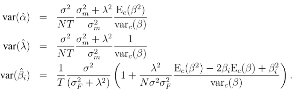
The standard errors of the maximum likelihood estimatorsαˆ,ˆλ, andβˆare:
var( ˆα) = 1 T σ2 F +λ2 σ2 F β′Ω−1 ε β (1′Ω−1 ε 1)(β′Ω−ε1β)−(1′Ω−ε1β)2 (8) var(ˆλ) = 1 T σ2 F +λ2 σ2 F 1′Ω−1 ε 1 (1′Ω−1 ε 1)(β′Ω−ε1β)−(1′Ω−ε1β)2 (9) var( ˆβ) = 1 T 1 λ2+σ2 F × [ Ω + λ 2 σ2 F (β′Ω−1 ε β)11′−(1′Ω−ε1β)β1′−(1′Ω−ε1β)1β′+ (1′Ω−ε11)ββ′ (1′Ω−1 ε 1)(β′Ω−ε1β)−(1′Ω−ε1β)2 ] . (10)
We provide a full derivation in Appendix A.
To obtain some intuition, consider the case where idiosyncratic risk is uncorrelated across stocks so Ωε is diagonal with elements{σi2}. We define the following cross-sectional sample
moments, which we denote with a subscript cto emphasize they are cross-sectional moments and the summations are acrossN stocks:
Ec(β/σ2) = 1 N ∑ j βj σ2 j Ec(β2/σ2) = 1 N ∑ j β2 j σ2 j Ec(1/σ2) = 1 N ∑ j 1 σ2 j varc(β/σ2) = ( 1 N ∑ j β2 j σ4 j ) − ( 1 N ∑ j βj σ2 j )2 covc(β2/σ2,1/σ2) = ( 1 N ∑ j β2 j σj4 ) − ( 1 N ∑ j β2 j σj2 ) ( 1 N ∑ j 1 σj2 ) . (11)
In the case of uncorrelated idiosyncratic risk across stocks, the standard errors ofαˆ,λˆ, and
ˆ βi in equations (8)-(10) simplify to var( ˆα) = 1 N T σ2 F +λ2 σ2 F Ec(β2/σ2) varc(β/σ2)−covc(β2/σ2,1/σ2) (12) var(ˆλ) = 1 N T σ2 F +λ2 σ2 F Ec(1/σ2) varc(β/σ2)−covc(β2/σ2,1/σ2) (13) var( ˆβi) = 1 T σ2 i (σ2 F +λ2) ( 1 + λ 2 N σ2 iσ2F Ec(β2/σ2)−2βiEc(β/σ2) +βi2Ec(1/σ2) varc(β/σ2)−covc(β2/σ2,1/σ2) ) .(14)
Comment 2.1 The standard errors ofαˆ and λˆ depend on the cross-sectional distributions of betas and idiosyncratic volatility.
In equations (12) and (13), the cross-sectional distribution of betas scaled by idiosyncratic variance determines the standard errors of αˆ and ˆλ. Some intuition for these results can be gained from considering a panel OLS regression with independent observations exhibiting het-eroskedasticity. In this case GLS is optimal, which can be implemented by dividing the re-gressor and regressand of each observation by residual standard deviation. This leads to the variances of αˆ and λˆ involving moments of 1/σ2. Intuitively, scaling by 1/σ2 places more
weight on the asset betas estimated more precisely, corresponding to those stocks with lower idiosyncratic volatilities. Unlike standard GLS, the regressors are estimated and the parameters
βi andλenter non-linearly in the data generating process (1). Thus, one benefit of using
max-imum likelihood to compute standard errors to measure efficiency losses of portfolios is that it takes into account the errors-in-variables of the estimated betas.
Comment 2.2 Cross-sectional and time-series data are useful for estimatingαandλbut pri-marily only time-series data is useful for estimatingβi.
In equations (12) and (13), the variance ofαˆandλˆdepend onN andT. Under the IID error assumption, increasing the data by one time period yields another N cross-sectional observa-tions to estimateαandλ. Thus, the standard errors follow the same convergence properties as a pooled regression with IID time-series observations, as noted by Cochrane (2001). In contrast, the variance ofβˆi in equation (14) depends primarily on the length of the data sample,T. The
stock beta is specific to an individual stock, so the variance ofβˆiconverges at rate1/T and the
convergence ofβˆi to its population value is not dependent on the size of the cross section. The
standard error ofβˆidepends on a stock’s idiosyncratic variance,σi2, and intuitively stocks with
smaller idiosyncratic variance have smaller standard errors forβˆi.
The cross-sectional distribution of betas and idiosyncratic variances enter the variance of
ˆ
βi, but the effect is second order. Equation (14) has two terms. The first term involves the
idiosyncratic variance for a single stocki. The second term involves cross-sectional moments of betas and idiosyncratic volatilities. The second term arises because α andλ are estimated, and the sampling variation of αˆ and λˆ contributes to the standard error of βˆi. Note that the
second term is of order1/N and when the cross section is large enough is approximately zero.6
Comment 2.3 Sampling error of the factor loadings affects the standard errors ofαˆandˆλ. Appendix A shows that the term(σ2F +λ2)/σ2F in equations (12) and (13) arises through the estimation of the betas. This term is emphasized by Gibbons, Ross and Shanken (1989) and Shanken (1992) and takes account of the errors-in-variables of the estimated betas. If H0λ=µ
holds andλ=µ, then this term reduces to the squared Sharpe ratio, which is given a geometric interpretation in mean-variance spanning tests by Huberman and Kandel (1987).
2.4
Portfolios and Factor Loadings
From the properties of maximum likelihood, the estimators using all stocks are most efficient with standard errors given by equations (12)-(14). If we use onlyP portfolios as test assets, what is the efficiency loss? Let the portfolio weights beϕpi, where p= 1, . . . , P andi= 1, . . . , N.
The returns for portfoliopare given by:
Rpt =α+βpλ+βpFt+σpεpt, (15)
where we denote the portfolio returns with a superscriptpto distinguish them from the under-lying securities with subscriptsi,i= 1, . . . , N, and
βp = ∑ i ϕpiβi σp = ( ∑ i ϕ2piσi2 )1/2 (16)
in the case of no cross-sectional correlation in the residuals.
The literature forming portfolios as test assets has predominantly used equal weights with each stock assigned to a single portfolio (see for example, Fama and French, 1993; Jagannathan and Wang, 1996). Typically, each portfolio contains an equal number of stocks. We follow this practice and formP portfolios, each containingN/P stocks with ϕpi = P/N for stock i
belonging to portfoliopand zero otherwise. Each stock is assigned to only one portfolio usually based on an estimate of a factor loading or a stock-specific characteristic.
ˆ
α9αandλˆ9λasN→ ∞. The maximum likelihood estimators are onlyT-consistent in line with a standard Weak Law of Large Numbers. WithT fixed,λˆis estimated ex post, which Shanken (1992) terms an ex-post price of risk. AsN→ ∞,ˆλconverges to the ex-post price of risk. Only asT → ∞doesαˆ→αandλˆ→λ.
2.5
The Approach of Fama and French (1992)
An approach that uses all individual stocks but computes betas using test portfolios is Fama and French (1992). Their approach seems to have the advantage of more precisely estimated factor loadings, which come from portfolios, with the greater efficiency of using all stocks as observations. Fama and French run cross-sectional regressions using all stocks, but they use portfolios to estimate factor loadings. First, they createP portfolios and estimate betas,βˆp, for
each portfolio p. Fama and French assign the estimated beta of an individual stock to be the fitted beta of the portfolio to which that stock is assigned. That is,
ˆ
βi = ˆβp ∀i∈p. (17)
The Fama-MacBeth (1973) cross-sectional regression is then run over all stocks i = 1, . . . , N
but using the portfolio betas instead of the individual stock betas. In Appendix D we show that in the context of estimating only factor risk premia, this procedure results in exactly the same risk premium coefficients as running a cross-sectional regression using the portfoliosp= 1, . . . , P
as test assets. Thus, estimating a pure factor premium using the approach of Fama and French (1992) on all stocks is no different from estimating a factor model using portfolios as test assets. Consequently, our treatment of portfolios nests the Fama and French (1992) approach.
2.6
Intuition Behind Efficiency Losses Using Portfolios
Since the maximum likelihood estimates achieve the Cram´er-Rao lower bound, creating subsets of this information can only do the same at best and usually worse.7 In this section, we present
the intuition for why creating portfolios leads to higher standard errors than using all individual stocks. To illustrate the reasoning most directly, assume thatσi = σ is the same across stocks
and the idiosyncratic shocks are uncorrelated across stocks. In this case the standard errors of
7Berk (2000) also makes the point that the most effective way to maximize the cross-sectional differences in expected returns is to not sort stocks into groups. However, Berk focuses on first forming stocks into groups and then running cross-sectional tests within each group. In this case the cross-sectional variance of expected returns within groups is lower than the cross-sectional variation of expected returns using all stocks. Our results are different because we consider the efficiency losses of using portfolios created from all stocks, rather than just using stocks or portfolios within a group.
ˆ
α,λˆ, andβˆi in equations (8)-(10) simplify to
var( ˆα) = σ 2 N T σ2m+λ2 σ2 m Ec(β2) varc(β) var(ˆλ) = σ 2 N T σ2m+λ2 σ2 m 1 varc(β) var( ˆβi) = 1 T σ2 (σ2 F +λ2) ( 1 + λ 2 N σ2σ2 F Ec(β2)−2βiEc(β) +βi2 varc(β) ) . (18)
Assume that beta is normally distributed. We create portfolios by partitioning the beta space intoP sets, each containing an equal proportion of stocks. We assign all portfolios to have1/P
of the total mass. Appendix E derives the appropriate moments for equation (18) when using
P portfolios. We refer to the variance ofαˆ andˆλcomputed usingP portfolios as varp( ˆα)and
varp(ˆλ), respectively, and the variance of the portfolio beta,βp, as var( ˆβp).
The literature’s principle motivation for grouping stocks into portfolios is that “estimates of market betas are more precise for portfolios” (Fama and French, 1993, p430). This is true and is due to the diversification of idiosyncratic risk in portfolios. In our setup, equation (14) shows that the variance for βˆi is directly proportional to idiosyncratic variance, ignoring the small
second term if the cross section is large. This efficiency gain in estimating the factor loadings is tremendous.
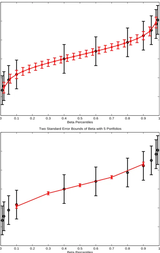
Figure 1 considers a sample size ofT = 60 withN = 1000 stocks under a single factor model where the factor shocks are Ft ∼ N(0,(0.15)2/12) and the factor risk premium λ =
0.06/12. We graph various percentiles of the true beta distribution with black circles. For individual stocks, the standard error of βˆi is 0.38 assuming that betas are normally distributed
with mean 1.1 and standard deviation 0.7 with σ = 0.5/√12. We graph two-standard error bands of individual stock betas in black through each circle. When we create portfolios, var( ˆβp)
shrinks by approximately the number of stocks in each portfolio, which isN/P. The top plot of Figure 1 shows the position of theP = 25portfolio betas, which are plotted with small crosses linked by the red solid line. The two-standard error bands for the portfolio betas go through the red crosses and are much tighter than the two-standard error bands for the portfolios. In the bottom plot, we show P = 5portfolios with even tighter two-standard error bands where the standard error ofβˆp is 0.04.
However, this substantial reduction in the standard errors of portfolio betas does not mean that the standard errors ofαˆandλˆare lower using portfolios. In fact, aggregating information into portfolios increases the standard errors ofαˆandˆλ. Grouping stocks into portfolios has two effects on var( ˆα)and var(ˆλ). First, the idiosyncratic volatilities of the portfolios change. This
does not lead any efficiency gain for estimating the risk premium. Note that the term σ2/N
using all individual stocks in equation (18) remains the same using P portfolios since each portfolio contains equal mass1/P of the stocks:
σ2 p P = (σ2P/N) P = σ2 N. (19)
Thus, when idiosyncratic risk is constant, forming portfolios shrinks the standard errors of factor loadings, but this has no effect on the efficiency of the risk premium estimate. In fact, the formulas (18) involve the total amount of idiosyncratic volatility diversified by all stocks and forming portfolios does not change the total composition.8 Equation (19) also shows that
it is not simply a denominator effect of using a larger number of assets for individual stocks compared to using portfolios that makes using individual stocks more efficient.
The second effect in forming portfolios is that the cross-sectional variance of the portfolio betas, varc(βp), changes compared to the cross-sectional variance of the individual stock betas,
varc(β). Forming portfolios destroys some of the information in the cross-sectional dispersion
of beta making the portfolios less efficient. When idiosyncratic risk is constant across stocks, the only effect that creating portfolios has on var(ˆλ)is to reduce the cross-sectional variance of beta compared to using all stocks, that is varc(βp) < varc(β). Figure 1 shows this effect. The
cross-sectional dispersion of theP = 25betas is similar to, but smaller than, the individual beta dispersion. In the bottom plot, the P = 5portfolio case clearly shows that the cross-sectional variance of betas has shrunk tremendously. It is this shrinking of the cross-sectional dispersion of betas that causes var( ˆα)and var(ˆλ)to increase when portfolios are used.
Our analysis sofar forms portfolios on factor loadings. Often in practice, and as we inves-tigate in our empirical work, coefficients on firm-level characteristics are estimated as well as coefficients on factor betas.9 We show in Appendix B that the same results hold for estimating
the coefficient on a firm-level characteristic using portfolios versus individual stocks. Grouping stocks into portfolios destroys cross-sectional information and inflates the standard error of the cross-sectional coefficients.
8Kandel and Stambaugh (1995) and Grauer and Janmaat (2008) show that repackaging the tests assets by linear transformations ofN assets intoN portfolios does not change the position of the mean-variance frontier. In our case, we formP < Nportfolios, which leads to inefficiency.
9We do not focus on the question of the most powerful specification test of the factor structure in equation (1) (see, for example, Daniel and Titman, 1997; Jagannathan and Wang, 1998; Lewellen, Nagel and Shanken, 2010) or whether the factor lies on the efficient frontier (see, for example, Roll and Ross, 1994; Kandel and Stambaugh, 1995). Our focus is on testing whether the model intercept term is zero,Hα=0
0 , whether the factor is priced given
the model structure,Hλ=0
0 , and whether the factor cross-sectional mean is equal to its time-series average,H
λ=µ
What drives the identification ofα andλ is the cross-sectional distribution of betas. Intu-itively, if the individual distribution of betas is extremely diverse, there is a lot of information in the betas of individual stocks and aggregating stocks into portfolios causes the information contained in individual stocks to become more opaque. Thus, we expect the efficiency losses of creating portfolios to be largest when the distribution of betas is very disperse.
3
Data and Efficiency Losses
In our empirical work, we use first-pass OLS estimates of betas and estimate risk premia coef-ficients in a second-pass cross-sectional regression. We work in non-overlapping five-year pe-riods, which is a trade-off between a long enough sample period for estimation but over which an average true (not estimated) stock beta is unlikely to change drastically (see comments by Lewellen and Nagel, 2006; Ang and Chen, 2007). Our first five-year period is from January 1961 to December 1965 and our last five-year period is from January 2001 to December 2005. We consider each stock to be a different draw from equation (1). Our data are sampled monthly and we take all stocks listed on NYSE, AMEX, and NASDAQ with share type codes of 10 or 11. In order to include a stock in our universe it must be traded at the end of each five-year period with price above $1 and market capitalization of at least $1 million. Each stock must have data for at least three out of five years. Our stock returns are in excess of the Ibbotson one-month T-bill rate. In our empirical work we use regular OLS estimates of betas over each five-year period. Our simulations also follow this research design and specify the sample length to be 60 months.
We estimate a one-factor market model using the CRSP universe of individual stocks or using portfolios. Our empirical strategy mirrors the data generating process (1) and looks at the relation between realized factor loadings and realized average returns. We take the CRSP value-weighted excess market return to be the single factor. We do not claim that the uncondi-tional CAPM is appropriate or truly holds, rather our purpose is to illustrate the differences on parameter estimates and the standard errors ofαˆandλˆwhen the entire sample of stocks is used compared to creating test portfolios.
3.1
Distribution of Betas and Idiosyncratic Volatility
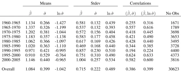
Table 2 reports summary statistics of the betas and idiosyncratic volatilities across firms. The full sample contains 30,623 firm observations. As expected, betas are centered approximately at
one, but are slightly biased upwards due to smaller firms tending to have higher betas. The cross-sectional beta distribution has a mean of 1.08 and a cross-cross-sectional standard deviation of 0.72. The average annualized idiosyncratic volatility is 0.40 with a cross-sectional standard deviation of 0.22. Average idiosyncratic volatility has generally increased over the sample period from 0.27 over 1960-1965 to 0.53 over 1995-2000, as Campbell et al. (2001) find, but it declines at the end of 2005 to 0.44 consistent with Bekaert, Hodrick and Zhang (2010). Stocks with high idiosyncratic volatilities tend to be stocks with high betas, with the correlation between beta andσequal to 0.39.
In Figure 2, we plot empirical histograms of beta (top panel) andlnσ (bottom panel) over all firm observations. The distribution of beta is positively skewed, with a skewness of 0.89, and fat-tailed with an excess kurtosis of 3.50. This implies there is valuable cross-sectional dis-persion information in the tails of betas which forming portfolios may destroy. The distribution oflnσis fairly normal, with almost zero skew at 0.18 and excess kurtosis of -0.01.
3.2
Efficiency Losses Using Portfolios
We compute efficiency losses usingP portfolios compared to individual stocks using the vari-ance ratios
varp( ˆα)
var( ˆα) and
varp(ˆλ)
var(ˆλ), (20)
where we denote the variances ofαˆ and ˆλcomputed using portfolios as varp( ˆα)and varp(ˆλ),
respectively. We compute these variances using Monte Carlo simulations allowing for progres-sively richer stochastic environments. First, we allow variation in idiosyncratic volatility to be cross-sectionally correlated with betas, but form portfolios based on true, not estimated, betas. Second, we form portfolios based on estimated betas. Third, we specify that firms with high betas tend to have high idiosyncratic volatility, as is observed in data. Finally, we allow entry and exit of firms in the cross section. We show that each of these variations further contributes to efficiency losses when using portfolios compared to individual stocks.
3.2.1 Cross-Sectionally Correlated Betas and Idiosyncratic Volatility Consider the following one-factor model at the monthly frequency:
whereεit ∼N(0, σ2i). We specify the factor returns Ft ∼ N(0,(0.15)2/12), λ = 0.06/12and
specify a joint normal distribution for(βi, lnσi):
( βi lnσi ) ∼N (( 1.08 −2.27 ) , ( 0.51 0.14 0.14 0.34 )) , (22)
which implies that the cross-sectional correlation between betas andlnσi is 0.43. These
param-eters come from the one-factor betas and residual risk volatilities reported in Table 1. From this generated data, we compute the standard errors ofαˆandλˆin the estimated process (1), which are given in equations (12) and (13).
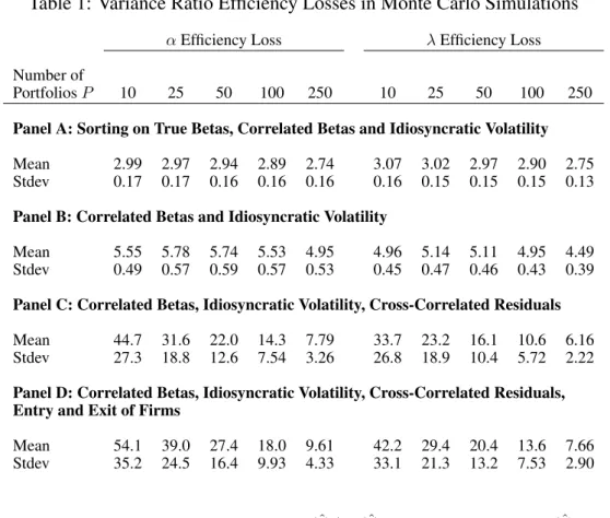
We simulate small samples of sizeT = 60months withN = 5000stocks. We use OLS beta estimates to form portfolios using the ex-post betas estimated over the sample. Note that these portfolios are formed ex post at the end of the period and are not tradable portfolios. In each simulation, we compute the variance ratios in equation (20). We simulate 10,000 small samples and report the mean and standard deviation of variance ratio statistics across the generated small samples. Table 1 reports the results. In all cases the mean and medians are very similar and the standard deviations of the variance ratios are very small at less than 1/10th the value of the mean or median.
Panel A of Table 1 formsP portfolios ranking on true betas and shows that forming as few as P = 10 portfolios leads to variances of the estimators 3.0 and 3.1 times larger for αˆ and
ˆ
λ, respectively. Even when 250 portfolios are used, the variance ratios are still around 2.7 for bothαˆandˆλ. The large variance ratios are due to the positive correlation between idiosyncratic volatility and betas in the cross section. Creating portfolios shrinks the absolute value of the
−covc(β2/σ2,1/σ2)term in equations (12) and (13). This causes the standard errors ofαˆ and
ˆ
λ to significantly increase using portfolios relative to the case of using all stocks. When the correlation of beta and lnσ is set higher than our calibrated value of 0.43, there are further efficiency losses from using portfolios.
Forming portfolios based on true betas yields the lowest efficiency losses; the remaining panels in Table 1 form portfolios based on estimated betas.10 In Panel B, where we form
portfolios on estimated betas with the same data-generating process as Panel A, the efficiency losses increase. For P = 25portfolios the mean variance ratio varp(ˆλ)/var(ˆλ)is 5.1 in Panel
B compared to 3.0 in Panel A when portfolios are formed on the true betas. ForP = 250
port-10We confirm Shanken and Zhou (2007) that the maximum likelihood estimates are very close to the two-pass cross-sectional estimates and portfolios formed on maximum likelihood estimates give very similar results to portfolios formed on the OLS betas.
folios formed on estimated betas, the mean variance ratio forˆλis still 4.5. Thus, the efficiency losses increase considerably once portfolios are formed on estimated betas. More sophisti-cated approaches to estimating betas, such as Avramov and Chordia (2006) and Meng, Hu and Bai (2007), do not make the performance of using portfolios any better because these methods can be applied at both the stock and the portfolio level.
When betas are estimated, the cross section of estimated betas is wider, by sampling error, than the cross section of true betas. These estimation errors are diversifiable in portfolios, which is why theP = 10portfolio variance ratios are slightly lower than the moderately largeP = 25
or P = 50 cases. For example, the variance ratio for λˆ is 5.0 for P = 10 when we sort on estimated betas, but 5.1 usingP = 25portfolios. Interestingly, the efficiency losses are greatest for P = 25 portfolios, which is a number often used in empirical work. As the number of portfolios further increases, the diversification of beta estimation error becomes minimal, but this is outweighed by the increasing dispersion in the cross section of (noisy) betas causing the variance ratios to decrease. These two offsetting effects cause the slight hump-shape in the variance ratios in Panel B.
3.2.2 Cross-Sectionally Correlated Residuals
We now extend the simulations to account for cross-sectional correlation in the residuals. We extend the data generating process in equation (21) by assuming
εit=ξiut+σvivit, (23)
where ut ∼ N(0, σu2) is a common, zero-mean, residual factor that is not priced and vit is a
stock-specific shock. This formulation introduces cross-sectional correlation across stocks by specifying each stockito have a loading,ξi, on the common residual shock,ut.
To simulate the model we draw(βiξi lnσvi)from
βi ξi lnσvi ∼N 1.08 1.02 −2.28 , 0.51 0.24 0.14 0.24 1.38 0.30 0.14 0.30 0.24 , (24) and set σu = 0.09/ √
12. In this formulation, stocks with higher betas tend to have residuals that are more correlated with the common shock (the correlation betweenβ andξ is 0.29) and higher idiosyncratic volatility (the correlation ofβwithlnσviis 0.40).
We report the efficiency loss ratios ofαˆandλˆin Panel C of Table 1. The loss ratios are an order of magnitude larger, on average, than Panels A and B and are 32 for varp( ˆα)/var( ˆα)and 23
for varp(ˆλ)/var(ˆλ)forP = 25portfolios. Thus, introducing cross-sectional correlation makes
the efficiency losses in using portfolios worse compared to the case with no cross-sectional correlation. The intuition is that cross-sectionally correlated residuals induces further noise in the estimated beta loadings. The increased range of estimated betas further reduces the dispersion of true portfolio betas.
3.2.3 Entry and Exit of Individual Firms
One reason that portfolios may be favored is that they permit analysis of a fixed cross section of assets with potentially much longer time series than individual firms. However, this particular argument is specious because assigning a stock to a portfolio must be made on some criteria; ranking on factor loadings requires an initial, “pre-ranking” beta to be estimated on individual stocks. If a firm meets this criteria, then analysis can be done at the individual stock level. Nevertheless, it is still an interesting and valid exercise to compute the efficiency losses using stocks or portfolios with a stochastic number of firms in the cross section.
We consider a log-logistic survivor function for a firm surviving to month T after listing given by
P(T > t) = [1 + ((0.0113)T)1.2658]−1, (25) which is estimated on all CRSP stocks taking into account right-censoring. The implied median firm duration is 31 months. We simulate firms over time and at the end of eachT = 60month period, we select stocks with at least T = 36 months of history. In order to have a cross section of 5,000 stocks, on average, with at least 36 observations, the average total number of firms is 6,607. We start with 6,607 firms and as firms delist, they are replaced by new firms. Firm returns follow the data-generating process in equation (21) and as a firm is born, its beta, common residual loading, and idiosyncratic volatility are drawn from equation (24).
Panel D of Table 1 reports the results. The efficiency losses are larger, on average, than Panel C with a fixed cross section. For example, with 25 portfolios, varp(ˆλ)/var(ˆλ) = 29
compared to 23 for Panel C. Thus, with firm entry and exit, forming portfolios results in greater efficiency losses. Although the number of stocks is, on average, the same as in Panel C, the cross section now contains stocks with fewer than 60 observations (but at least 36). This increases the estimation error of the betas, which accentuates the same effect as Panel B. There is now larger error in assigning stocks with very high betas to portfolios and creating the portfolios masks the true cross-sectional dispersion of the betas. In using individual stocks, the information in the beta cross section is preserved and there is no efficiency loss.
3.2.4 Summary
Potential efficiency losses are large for using portfolios instead of individual stocks. The effi-ciency losses become larger when residual shocks are cross-sectionally correlated across stocks and when the number of firms in the cross section changes over time.
4
Empirical Analysis
We now investigate the differences in using portfolios versus individual stocks in data. We com-pare estimates of a one-factor market model on the CRSP universe in Section 4.1 and the Fama-French (1993) three-factor model in Section 4.2. We compute standard errors using maximum likelihood, which assumes normally distributed residuals, and GMM, which is distribution free. The standard errors account for cross-correlated residuals, which are modeled by a common factor or using industry factors. This is described in Appendix F. We concentrate our discus-sion in the text below on the one-factor residual model – henceforth all references to maximum likelihood and GMM standard errors refer to those using the one-factor residual model. We note that the results using the industry classifications are similar. We present both models of residual correlation in the tables for completeness and as an additional robustness check. The coefficient estimates we report are all annualized by multiplying the monthly estimates by 12.
4.1
One-Factor Model
4.1.1 Using All Stocks
Panel A of Table 3 reports the estimates of α and λ in equation (1) using all 30,623 firm ob-servations. The factor model in equation (1) implies a relation between realized firm excess returns and realized firm betas. Thus, we stack all stocks’ excess returns from each five-year period into one panel and run a cross-sectional regression using average realized firm excess returns over each five-year period as the regressand and with a constant and the estimated betas as regressors. Table 3 reports both maximum likelihood and GMM standard errors taking into account cross-sectional residual correlation.
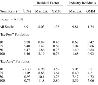
Using all stocks produces estimates of αˆ = 5.40% and λˆ = 6.91%. The maximum like-lihood standard errors for both estimates are 0.14, with t-statistics of 40 and 48, respectively. The GMM standard errors do not assume normally distributed residuals and this reduces the t-statistics to 5.6 and 8.3, respectively. Thus, the CAPM is firmly rejected since H0α=0 is
over-whelmingly rejected. While the CAPM is rejected, we clearly also reject Hλ=0
0 , and so the
market factor is priced. In fact, over 1961-2005, the market excess return isµ= 5.76%, which is close to the cross-sectional estimateλˆ= 5.40%. We formally testH0λ=µbelow.
Even using GMM, the t-statistics in Panel A are fairly large compared to most of the litera-ture. This is due to two main reasons. First, we test the relation of realized returns with realized betas over the same sample period on individual stocks. The magnitudes of these t-statistics are comparable to other studies with the same the experimental design like Ang, Chen and Xing (2006). Second, the literature often reports t-statistics using portfolios, particularly port-folios sorted on predicted rather than realized betas. Our theoretical results show there should be a potentially large loss of efficiency in using portfolios. We are interested not so much in the differences across the various standard errors (maximum likelihood versus GMM), but rather in the increase in the standard errors, or the decrease in the absolute values of the t-statistics, resulting from using portfolios rather than individual stocks as test assets. We now investigate these effects.
4.1.2 “Ex-Post” Portfolios
We form “ex-post” portfolios in Panel B of Table 3. Over each five-year period we group stocks into P portfolios based on realized OLS estimated betas over those five years. All stocks are equally weighted at the end of the five-year period within each portfolio. While these portfolios are formed ex post and are not tradeable, they represent valid test assets to estimate the cross-sectional model (1). In all cases,αˆandˆλestimated using the ex-post portfolios are remarkably close to the estimates computed using all stocks.
As expected, the maximum likelihood standard errors using portfolios are much larger than the standard errors computed using all stocks. For example, forP = 25portfolios the maximum likelihood standard error onˆλis 0.46 compared with 0.14 using all stocks. AsP increases, the standard errors decrease (and the t-statistics increase) to approach the values using individual stocks. The differences in standard errors for GMM in using portfolios versus individual stocks are smaller, but still significant. For example, for P = 25portfolios the GMM standard error forˆλis 1.04, with a t-statistic of 6.1, compared with a standard error of 0.84 and a t-statistic of 8.3 for all stocks. Thus, forming portfolios ex post results in appreciable losses of efficiency.
The last three columns of Table 3 report statistics of the cross-sectional dispersion of beta: the cross-sectional standard deviation,σc( ˆβ), and the beta values corresponding to the 5%- and
distri-bution of beta in creating the ex-post portfolios. Over all stocks, the cross-sectional standard deviation of beta σc( ˆβ) = 0.71. For P = 25 ex-post portfolios, the cross-sectional standard
deviation of beta isσc( ˆβp) = 0.69. Maximum likelihood is more sensitive to the betas in the
tails and this causes the large increase in the maximum likelihood standard errors when using portfolios. GMM is less sensitive to this small shrinking of the cross-sectional beta distribution, but there are still significant increases in the GMM standard errors when portfolios are used.
4.1.3 “Ex-Ante” Portfolios
In Panel C of Table 3 we form “ex-ante” tradeable portfolios. We group stocks into portfolios at the beginning of each calendar year ranking on the market beta estimated over the previous five years. Equally-weighted portfolios are created and the portfolios are held for twelve months to produce portfolio returns. The portfolios are rebalanced annually. The sample period and the set of stocks in the ex-ante portfolios at each time are the same as Panels A and B. After the ex-ante portfolios are created, we compute realized OLS market betas of each portfolio in each non-overlapping five-year period and then run a second-pass cross-sectional regression to estimateαandλ. Thus, we examine the same realized beta–realized return relation as in Panels A and B, except the test portfolios are different.
Panel C shows the estimates ofαandλfrom these ex-ante portfolios are very dissimilar to the estimates in Panels A and B. Using the ex-ante portfolios produces an estimate ofαaround 12-13% and an estimate of λ that is negative, but close to zero. In contrast, both the all stock case (Panel A) and the ex-post portfolios (Panel B) produce positive alpha estimates around 5% and estimates ofλaround 6-7%. Theλestimates have relatively large standard errors compared to the full stock universe and the ex-post portfolios. For example, the GMM standard error of
ˆ
λ forP = 25 ex-ante portfolios is 1.87 compared to 0.84 for all stocks and 1.04 forP = 25
ex-post portfolios. Thus, while Hα=0
0 is always rejected, the ex-ante portfolios fail to reject
Hλ=0
0 , which is overwhelmingly rejected using all stocks and the ex-post portfolios.
The ex-ante portfolios produce such a markedly differentαˆ andλˆbecause ranking on pformation betas dramatically shrinks the post-pformation realized distribution of beta. It is the re-alized distribution of betas that is important for testing the factor model. The last three columns of Table 3, Panel C show the shrinking dispersion of the cross section of betas compared to all stocks in Panel A and the ex-post portfolios in Panel B. For P = 25 ex-post portfolios, the cross-sectional standard deviation of beta is onlyσc( ˆβp) = 0.37for the ex-post portfolios
remove a lot of information in the tails of the beta distribution, with the 5% and 95%-tiles for the beta distributions from the P = 25 ex-post portfolios being 0.50 and 1.71, respectively, compared to 0.11 and 2.32 for all stocks. In contrast, the ex-post portfolios in Panel B preserve most of the distribution of realized betas because the ex-post portfolios are created at the end of each period, rather than at the beginning of each year.
Figure 3 plots the estimates of λ using different numbers of ex-ante portfolios and the all stocks case. While the ex-ante portfolio estimates ofλconverge to the estimate using all stocks as the number of ex-ante portfolios increases, the convergence rate is slow. Even for 3000 or 4000 ex-ante portfolios, which contain only one or two stocks each, the λ estimates are still 3.98% and 5.15%, respectively, compared to λˆ = 6.91% for the full stock universe. Figure 3 shows that using only a few portfolios can severely affect the point estimates due to a pro-nounced shrinking of the distribution of betas.
4.1.4 Tests of Cross-Sectional and Time-Series Estimates
We end our analysis of the one-factor model by testingH0λ=µ, which tests equality of the cross-sectional risk premium and the time-series mean of the market factor portfolio. Table 4 presents the results. Using all stocks,λˆ = 6.91%is fairly close to the time-series estimate,µˆ = 5.76%, but the small standard errors of maximum likelihood causeH0λ=µto be rejected with a t-statistic of 8.0. With GMM standard errors, we fail to reject H0λ=µ with a t-statistic of 1.4. The ex-post portfolio estimates generally fail to reject H0λ=µ at the 5% level, with the exception of
P = 100 ex-post portfolios for maximum likelihood standard errors. In contrast, the ex-ante portfolios reject H0λ=µ for both maximum likelihood and GMM standard errors because the ex-ante portfolios produce point estimates ofλthat are close to zero.
4.1.5 Summary
Using GMM standard errors, we can summarize our results in the following table:
Portfolios All Stocks Ex-Post Ex-Ante
Hα=0
0 Reject Reject Reject
Hλ=0
0 Reject Reject Fail to Reject
H0λ=µ Fail to Reject Fail to Reject Reject
We overwhelmingly rejectH0α=0and hence the one-factor model using all stocks or portfolios. However, using all stocks or portfolios produces different estimates of cross-sectional risk
pre-mia. In particular, using all stocks we estimate αˆ = 5.40% and ˆλ = 6.91%and reject Hα=0 0
andHλ=0
0 . We fail to rejectH λ=µ
0 becauseλˆis close toµˆ = 5.76%. Ex-post portfolios preserve
most of the cross-sectional spread in betas and produce similar risk premium point estimates to the all stocks case, although with larger standard errors. In contrast, creating ex-ante portfolios, which rank on past estimated betas, severely pares the tails of the realized betas. This changes the point estimates of the cross-sectional risk premium,λˆ, to be slightly negative. Thus, we fail to reject H0λ=0 and do not find that the market factor is priced. Furthermore, for the ex-ante portfolios we rejectH0λ=µbecause the low estimate ofλ is very far from the time-series mean of the market factor.
4.2
Fama-French (1993) Model
This section estimates the Fama and French (1993) model:
Rit =α+βM KT ,iλM KT +βSM B,iλSM B +βHM L,iλHM L +σiεit, (26)
whereM KT is the excess market return,SM B is a size factor, andHM Lis a value/growth factor. We follow the same procedure as Section 4.1 in estimating the cross-sectional coef-ficients α, λM KT, λSM B, and λHM L by in non-overlapping five-year periods and stacking all
observations into one panel.
4.2.1 Factor Loadings
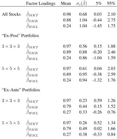
Panel A of Table 5 reports summary statistics of the distribution of the first-pass factor loadings
ˆ
βM KT,βˆSM B, andβˆHM L. Market betas are centered around one after controlling forSM Band
HM L. TheSM B andHM Lfactor loadings are not centered around zero even thoughSM B
andHM Lare zero-cost portfolios because the break points used by Fama and French (1993) to constructSM BandHM Lare based on NYSE stocks rather than on all stocks. Small stocks tend to skew the SM B and HM Lloadings to be positive, especially for the SM B loadings which have a mean of 0.88. Across all stocks, factor loadings of SM B and HM Lare more disperse than market betas, each with cross-sectional standard deviations of 1.04 compared to a cross-sectional standard deviation of 0.68 forβˆM KT.
We formn×n×nex-post portfolios by grouping stocks into equally-weighted portfolios based on realized estimated factor loadings at the end of the period. These are sequential sorts, sorting first onβˆM KT, then onβˆSM B, and lastly onβˆHM L. As a result, all portfolios contain the
portfolios at the beginning of each calendar year, ranking on the factor loadings estimated over the previous five years. The portfolios are held for twelve months to produce monthly portfolio returns, and are rebalanced annually at the beginning of each calendar year. We then compute realized OLS market betas of each portfolio in the same non-overlapping five-year periods as for the all stocks and ex-post portfolio cases, which are also used to run a second-pass cross-sectional regression to estimateαandλ.
Table 5 shows that the cross-sectional dispersion of the factor loadings decrease modestly for the ex-post portfolios. For example, for the5×5×5ex-post portfolios, theβˆSM B andβˆHM L
cross-sectional standard deviations are 0.95 and 0.94, respectively, compared to all stocks at 1.04 for both factor loadings. However, the ex-ante portfolios shrink the cross-sectional devia-tion by more than half compared to the all stock case. TheSM BandHM Lfactor loadings for the ex-ante5×5×5portfolios have cross-sectional standard deviations of only 0.49 and 0.38, respectively, compared to around 1.04 for for both factor loadings in all stocks. Furthermore, the ex-ante portfolios significantly reduce the left-hand tail ofHM Lfactor loadings, with the 5%-tile forβˆHM L going from -1.45 for all stocks to -0.33 for the5×5×5ex-ante portfolios.
Since the cross-sectional dispersion is so much smaller for the ante portfolios, we might ex-pect the second-pass cross-sectional factor risk premia estimates may be quite different for the ex-ante portfolios versus the estimates using all stocks and the ex-post portfolios. We now show this is indeed the case.
4.2.2 Cross-Sectional Factor Risk Premia
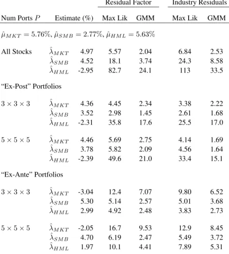
Table 6 reports estimates of the Fama-French (1993) factor risk premia. We rejectHα=0 0 with
both maximum likelihood and GMM standard errors in all three cases: using all stocks (Panel A), with the ex-post portfolios (Panel B), and the ex-ante portfolios (Panel C). In most cases, we also rejectHλ=0
0 for all factors. However, the point estimates and even the signs of the factor
risk premia change going from all stocks to the portfolio specifications.
Using all stocks in Panel A, we find a positive estimate of the market risk premium,ˆλM KT =
4.97%, which is consistent with the results of the one-factor model in Table 3, and a positive size factor premium,λˆSM B = 4.52%. However, we find a negative estimateˆλHM L =−2.95%
using all stocks. This is unexpected given the voluminous literature on the value premium and the positive time-series mean ofHM Lin data. The ex-post portfolios in Panel B have the same pattern with similar point estimates of the factor risk premia. This is consistent with the factor loadings in the ex-post portfolios having similar cross-sectional dispersion to the all stocks case
(see Table 5). In both Panels A and B, we overwhelmingly rejectHλ=0
0 for all three factors.
In contrast, the ex-ante portfolios in Panel C yield very different estimates of the Fama-French (1993) factor risk premia. Using3×3×3ex-ante portfolios, the market risk premium is now negative atˆλM KT =−3.04%with a maximum likelihood (GMM) t-statistic of 4.3 (2.4).
The size factor premium,λˆSM B = 5.30%, remains positive and is also highly significant. The
value factor premium is now positive,λˆHM L = 2.99%, and is significant with both maximum
likelihood and GMM standard errors. The positiveSM BandHM Lpremia are consistent with Fama and French (1992, 1993) and are similar using5×5×5ex-ante portfolios. Thus, the sign of the estimatedM KT andHM Lrisk premia depends on whether we use all stocks or ex-ante portfolios. Below, we explore this non-robustness further by including characteristic as well as factor loadings as regressors.
4.2.3 Tests of Cross-Sectional and Time-Series Estimates
Not surprisingly, the changing coefficients across all stocks and the ex-ante portfolios also af-fects the tests ofH0λ=µfor the Fama-French (1993) model. We report the results of these tests in Table 7. For the all stocks case in Panel A, we reject the hypothesis that the cross-sectional risk premia are equal to the mean factor portfolio returns. The maximum likelihood t-statistics are all above 5.5, though using GMM standard errors produces a t-statistic of 2.0 for testing
λM KT =µM KT, which is borderline significant at the 95% level. For the ex-post portfolios, we
firmly rejectH0λ=µin all cases except forSM Busing GMM standard errors. With the ex-ante portfolios, the hypothesis is also rejected in all cases, in part because of the large and negative estimate of λM KT. Thus, while the Fama-French (1993) factors are cross-sectionally priced,
there is little evidence that the cross-sectional risk premia are consistent with the time-series of factor returns.
4.2.4 HML Factor Loadings and Book-to-Market Characteristics
The negative HM Lpremium for the all stocks case is puzzling given the strong evidence on the book-to-market effect found in the literature. However, we show that high returns tend to accrue to stocks with high book-to-market ratios rather than stocks with highHM Lloadings, per se, as pointed out by Daniel and Titman (1997). In Table 8, we investigate the sign of the
HM Lrisk premium estimate in more detail. Here we consider stocks with observable market capitalization and book-to-market ratios. This makes our all stock universe slightly smaller than the full stock universe we previously considered in Tables 6 and 7.
In the top part of Panel A of Table 8, we report the risk premium estimates of the Fama-French (1993) model on this new universe. The results are qualitatively unchanged from Ta-ble 6: theM KT andSM Bpremia are strongly positive at 4.55% and 5.07%, respectively, and theHM Lpremium is negative at -2.85%. All three coefficients are all significant using either maximum likelihood or GMM standard errors. The risk premia estimates are similar to those in Table 6, which are 4.97%, 4.52%, and -2.95% forM KT,SM B, andHM L, respectively.
The second part of Panel A reports the estimates of a cross-sectional regression where the book-to-market ratio (B/M) is now included as an additional right-hand side variable. We mea-sure the book-to-market ratio at timet with fiscal year-end data for book-equity from the pre-vious year with timetmarket data. The cross-sectional regression is run using monthly returns over the next month with book-to-market ratios at time t. The factor loadings are estimated with first-pass time-series regressions in each five-year period and are the same as the factor loadings in the top part of Panel A. When we include the book-to-market ratio, the estimate of
λHM L continues to be negative, at -4.43%, but the coefficient on B/M is strongly positive at
7.93%. This finding is consistent with Daniel and Titman (1997): the book-to-market effect is a characteristic effect rather than a reward for bearingHM Lfactor loading risk.
In Panel B, we follow Fama and French (1993) and others by forming ex-ante portfolios based on characteristics rather than on factor loadings alone. We first create 5×5 portfolios sequentially sorted on market beta andB/M, rebalancing the portfolios annually at the begin-ning of each calendar year. Then we compute realized OLS market betas for each portfolio and estimate the factor risk premia in a second-pass cross-sectional regression. The cross-sectional coefficients have the same signs as the ex-ante portfolios of Panel C of Table 6. In particu-lar, the sign of the market risk premium is negative, at -8.15%, and bothλˆSM B = 12.5% and
ˆ
λHM L = 5.55% are positive. These three coefficients are significant at the 95% level using
maximum likelihood standard errors, except for the market risk premium, where the t-statistic is 1.92. Using GMM standard errors, only SMB is significant at the 95% level.
The bottom part of panel B shows that we also obtain a positive HM L premium if we estimate the cross-sectional regression on5×5ex-ante portfolios sequentially sorted on size and
B/M. In this case, theHM Lpremium becomes even larger at 8.81%. TheM KT andSM B
premia are now insignificantly different from zero using GMM standard errors. In summary, we obtain the more familiar result that theHM Lpremium is positive only on the more widely used ex-ante portfolios which sort stocks directly on the book-to-market characteristic (as in Fama and French, 1993). The book-to-market ratio is significantly positively related to returns, and