Performance Testing and
Performance Improvement
Methods for Communicating
Systems
Levente Er˝
os
MSc. in Technical InformaticsDepartment of Telecommunications and Media Informatics Doctoral School of Informatics
Faculty of Electrical Engineering and Informatics Budapest University of Technology and Economics
PhD. Dissertation
Supervised by: Dr. Tibor Cs¨ondes Honorary Associate Professor
Department of Telecommunications and Media Informatics Faculty of Electrical Engineering and Informatics Budapest University of Technology and Economics
Budapest, Hungary 2012.
Abstract
In this thesis, I propose methods for solving yet unsolved problems of black-box performance testing of communicating systems. The main motivation of creating the presented methods was the fact that while black-box conformance testing has evolved methods for test generation and execution, black-box performance testing lacks such methods, and performance tests are designed in an ad-hoc way.
The thesis has three main parts. The first two parts focus on two different aspects of performance testing, while the third part discusses a problem, which is based on the second part.
In the first part of the thesis, I deal with a problem of performance test execution namely, how to assign load generating software entities to the hosts of the perfor-mance test environment in order to exploit the capacities of the test environment as much as possible. After proving the NP-completeness of the problem, I formulate it as an integer linear program, and propose two heuristic methods for solving it. Then, the efficiency of the proposed methods are evaluated.
In the second part, I focus on a more specific case of performance testing in which, the performance requirement that the system under test (SUT) has to fulfill is the number of request messages to be processed within a second while serving a given number of users. I propose a performance testing method, which automati-cally checks whether the SUT fulfills this performance requirement. The presented method builds on the functional modeling techniques used in conformance testing. I compare the accuracy of the proposed method to that of an ad-hoc performance testing method used in the industry.
The third part of the thesis deals with the problem of increasing the performance of the SUT in case it has failed to pass the performance testing method presented in the second part of the thesis. After proving the NP-completeness of the problem, I formulate it as an integer linear program, and propose a heuristic algorithm for solving it. I also evaluate the efficiency of the two methods.
Kivonat
Disszert´aci´omban kommunik´al´o rendszerek fekete doboz alap´u teljes´ıtm´enytesztel´e-s´enek megoldatlan probl´em´aival foglalkozom. M´ıg a fekete doboz alap´u konformanci-atesztel´es kiforrott tesztgener´al´o ´es -v´egrehajt´o elj´ar´asokkal b´ır, a fekete doboz alap´u teljes´ıtm´enytesztel´esr˝ol ez nem mondhat´o el, s ´ıgy a teljes´ıtm´eny-tesztek tervez´ese ad-hoc m´odon t¨ort´enik. A bemutatott elj´ar´asok kidolgoz´as´anak motiv´aci´oja pon-tosan ez, azaz a kommunik´al´o rendszerek fekete doboz alap´u teljes´ıtm´enytesztel´ese elm´eleti h´atter´enek kifejletlens´ege.
A disszert´aci´o h´arom f˝o r´eszb˝ol ´all. Az els˝o k´et r´esz a teljes´ıtm´eny-tesztel´es k´et k¨ul¨onb¨oz˝o ter¨ulet´evel foglalkozik, m´ıg a harmadik r´eszben egy, a m´asodik r´eszben t´argyalt elj´ar´asra ´ep¨ul˝o probl´em´at mutatok be.
Az ´ertekez´es els˝o r´esz´eben a teljes´ıtm´enyteszt-v´egrehajt´as egy olyan probl´em´a-j´aval foglalkozom, amely sor´an a tesztk¨ornyezet hosztjaihoz ´ugy kell hozz´arendelni a tesztelt rendszert terhel˝o forgalmat gener´al´o szoftverentit´asokat, hogy a tesztk¨or-nyezet szabad kapacit´asait min´el jobban kihaszn´aljuk. NP-teljess´eg´enek bel´at´as´at k¨ovet˝oen a probl´em´at fel´ırom eg´esz´ert´ek˝u line´aris programk´ent, illetve bemutatok k´et heurisztikus algoritmust a probl´ema megold´as´ara. V´eg¨ul ¨osszehasonl´ıtom a k´et ismertetett elj´ar´as hat´ekonys´ag´at.
A m´asodik r´eszben a teljes´ıtm´enytesztel´es egy specifikusabb eset´evel foglalko-zom, amikor is a tesztelt rendszerrel szemben t´amasztott teljes´ıtm´enyk¨ovetelm´eny a rendszer ´altal m´asodpercenk´ent feldolgozand´o k´er´es¨uzenetek sz´ama adott sz´am´u felhaszn´al´o p´arhuzamos kiszolg´al´asa mellett. Ismertetek egy teljes´ıtm´enytesztel´esi elj´ar´ast, amely k´epes annak automatikus ellen˝orz´es´ere, hogy a tesztelt rendszer megfelel-e a fent eml´ıtett k´et teljes´ıtm´enyk¨ovetelm´enynek. A bemutatott elj´ar´as a konformanciatesztel´es ter¨ulet´en haszn´alt funkcion´alis modellez´esi m´odszereken ala-pul. A szakasz v´eg´en a bemutatott elj´ar´as pontoss´ag´at egy, az iparban haszn´alt ad-hoc elj´ar´as´eval hasonl´ıtom ¨ossze.
teljes´ıtm´eny-tesz-tel´esi elj´ar´ason megbukott rendszerek teljes´ıtm´eny´enek korrekci´oj´aval foglalkozik. A probl´ema NP-teljess´eg´enek bebizony´ıt´as´at k¨ovet˝oen azt egy eg´esz´ert´ek˝u line´aris programk´ent ´ırom fel, illetve bemutatok egy heurisztikus algoritmust a probl´ema megold´as´ara. A szakaszt a bemutatott megold´asi elj´ar´asok hat´ekonys´ag´anak vizs-g´alat´aval z´arom.
Acknowledgments
First of all, I would like to thank my supervisors, Dr. Tibor Cs¨ondes for all the time and energy he has put into consulting me and guiding my research work all through the past years, and Dr. Sarolta Dibuz for her useful advices and support.
I am also very grateful to Dr. Gyula Csopaki for inviting me to research the field of testing as an MSc student and for his continuous guidance and support.
Furthermore, I would like to thank my colleagues and roommates, Dr. P´eter Babarczi, G´abor ´Arp´ad N´emeth, and Zolt´an Nov´ak for their unconditional help and the great work athmosphere they provided. I would also like to thank my colleague, J´ozsef Ern˝o Marton, for his technical advices.
Also, I would like to thank the High Speed Networks Laboratory (HSNLab) for providing the technical and financial background for my research work, especially Dr. R´obert Szab´o, Dr. Attila Vid´acs, and Dr. S´andor Moln´ar for their useful advices related to my publications, and Erzs´ebet Gy˝ori for all her help.
My acknowledgments would not be complete without also thanking my head of department Dr. Tam´as Henk, Dr. Edit Hal´asz, Prof. Dr. Gyula Sallai, Dr. Guszt´av Adamis, and Dr. G´abor Kov´acs for their valuable advices on finalizing my thesis.
At last, but not at least I would like to thank all my family members for sup-porting me all through my student years, for the exceptional studying oppurtunities they provided, and for helping me overcome all the obstacles arisen.
Contents
1 Introduction 11
1.1 The Evolution of Conformance Testing . . . 12
1.2 Problems of Performance Testing . . . 14
2 Load Distribution in a Performance Testing Environment 17 2.1 Related Work . . . 18
2.2 Problem Definition and Complexity . . . 19
2.3 An ILP Based Heuristic Solution for the Load Distribution Problem . 22 2.4 A Bin Packing Based Heuristic Solution for the Load Distribution Problem . . . 27
2.5 Simulation Results . . . 29
2.6 Conclusions . . . 39
3 A Model-Driven Performance Testing Method for Communicating Systems 40 3.1 Related Work . . . 41
3.2 Performance Requirements and Motivations . . . 42
3.3 The Timed Communicating Finite Multistate Machine . . . 43
3.4 Creating the Test Execution Model . . . 46
3.5 Performance Evaluation . . . 49
3.5.1 Calculating the Worst-case Performance of the System Under Test . . . 50
3.5.2 Calculating the Expected Performance of the System Under Test . . . 55
3.6 Experimental Results . . . 58
4 Worst-Case Performance Correction of Communicating Systems 68
4.1 Definition of the Worst-Case Performance Correction Problem . . . . 69 4.2 Complexity of the Worst-case Performance Correction Problem . . . . 69 4.3 ILP formulation of the Worst-Case Performance Correction Problem . 73 4.4 A Heuristic Solution for the Worst-Case Performance Correction
Prob-lem . . . 74 4.5 Simulation Results . . . 81 4.6 Conclusions . . . 87
5 Summary and Future Work 88
5.1 Load Distribution in a Performance Testing Environment . . . 88 5.2 A Model-Driven Performance Testing Method for Communicating
Systems . . . 89 5.3 Worst-Case Performance Correction of Communicating Systems . . . 91
List of Figures
1.1 Development of communicating systems . . . 11
1.2 Manual (a), and script based (b) test design . . . 12
1.3 Model-based test design . . . 13
1.4 Performance testing . . . 15
2.1 Assigning THs to VHs . . . 17
2.2 Required capacity, |T H|= 3, TCavg = 60, StepTC = 0, ǫC = 4 . . . . 30
2.3 Average utilization, |T H|= 3, TCavg = 60, StepTC = 0, ǫC = 4 . . . . 31
2.4 Required capacity, |T H|= 3, TCavg = 60, StepTC = 0, ǫC = 20 . . . . 31
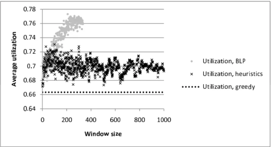
2.5 Average utilization, |T H|= 3, TCavg = 60, StepTC = 0, ǫC = 20 . . . 32
2.6 Required capacity, |T H|= 3, TCavg = 210, StepTC = 0, ǫC = 20 . . . 32
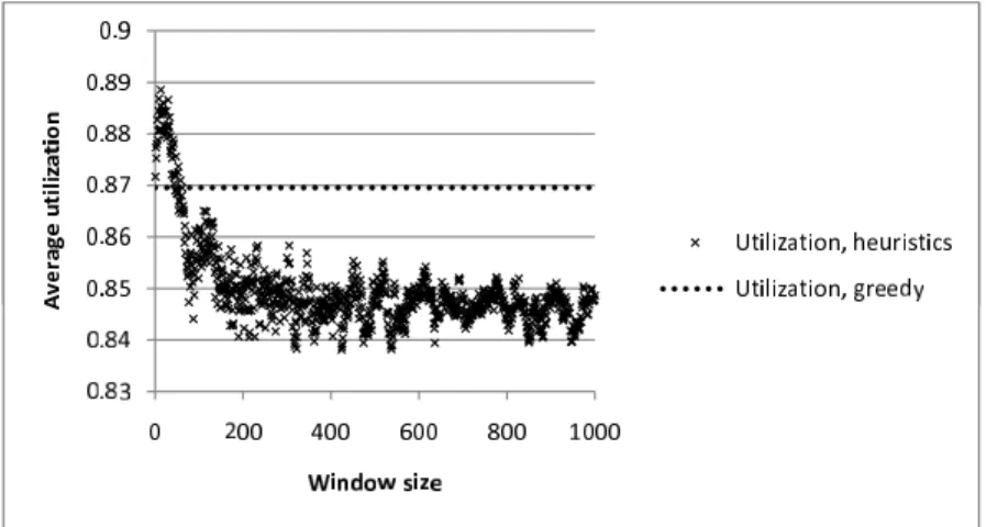
2.7 Average utilization, |T H|= 3, TCavg = 210, StepTC = 0, ǫC = 20 . . 33
2.8 Required capacity, |T H|= 3, TCavg = 60, StepTC = 5, ǫC = 20 . . . . 34
2.9 Average utilization, |T H|= 3, TCavg = 60, StepTC = 5, ǫC = 20 . . . 34
2.10 Required capacity, |T H|= 9, TCavg = 60, StepTC = 5, ǫC = 20 . . . . 35
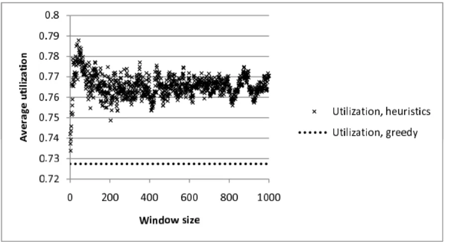
2.11 Average utilization, |T H|= 9, TCavg = 60, StepTC = 5, ǫC = 20 . . . 35
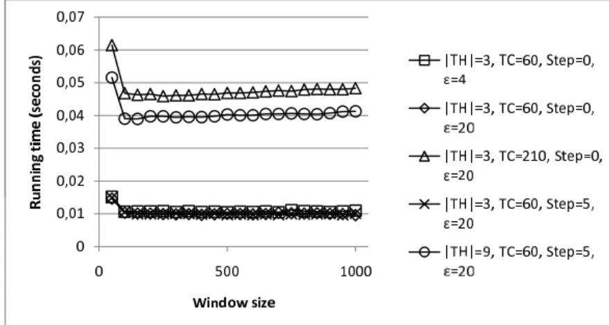
2.12 Running times of the ILP based algorithm . . . 36
2.13 Running times of the bin packing based algorithm . . . 36
2.14 Running times of the greedy algorithm . . . 37
3.1 Graphical representation of the TCFMM . . . 46
3.2 Redirecting sink transitions tos0 . . . 49
3.3 Experimental environment . . . 58
3.4 Measurements taken by the ad-hoc and the proposed method, in the first series of experiments . . . 61
3.5 Measurements of the ad-hoc method approachingCWusr, in the first series of experiments . . . 62
3.6 Deviation of measurements of the ad-hoc and the proposed method,
in the first series of experiments . . . 62
3.7 Histogram of M(1) used in the second series of experiments . . . 63
3.8 Measurements taken by the ad-hoc and the proposed method, in the second series of experiments . . . 64
3.9 Deviation of measurements of the ad-hoc and the proposed method, in the second series of experiments . . . 64
3.10 Histogram of M(1) used in the third series of experiments . . . 65
3.11 Measurements taken by the ad-hoc and the proposed method, in the third series of experiments . . . 65
3.12 Deviation of measurements of the ad-hoc and the proposed method, in the third series of experiments . . . 66
4.1 Costs of solutions,CWRusr = 1.0 . . . 83
4.2 Costs of solutions,CWRusr = 1.5 . . . 84
4.3 Costs of solutions,CWRusr = 1.75 . . . 85
4.4 Running times of the BLP . . . 86
4.5 Running times of the heuristics . . . 86
4.6 Running times of the LP . . . 86
List of Tables
2.1 Maximal average utilization values achieved by different methods in
different scenarios . . . 37
3.1 Measurement deviations of the ad-hoc and the proposed method, in the first series of experiments . . . 63
3.2 Measurement deviations of the ad-hoc and the proposed method, in the second series of experiments . . . 64
3.3 Measurement deviations of the ad-hoc and the proposed method, in the third series of experiments . . . 66
4.1 Costs of solutions,CWRusr = 1.0 . . . 83
4.2 Costs of solutions,CWRusr = 1.5 . . . 84
Chapter 1
Introduction
Testing plays a vital role in the development of a communicating system imple-menting a certain communication protocol. After the implementation phase, the developed system is regarded as a black box and different kinds of tests are exe-cuted against it in order to check whether it corresponds to its different kinds of requirements. Both the implementation and the testing phases use the specifica-tions of the System Under Test (SUT from now on) as their inputs (see Figure 1.1). The implementation phase has well-developed methodologies, but these are not covered in this thesis. In the testing phase, among many others, the fulfillment of the conformance and performance requirements of the SUT are tested. In the rest of this chapter, I am going to review the current state of the art regarding the level of automation in conformance testing and performance testing and identify some problems, which are related to performance testing and for which, I propose solutions in this thesis.
1.1
The Evolution of Conformance Testing
In the field of telecommunications, conformance testing investigates whether the SUT implements the communicating protocol that it should implement according to its conformance requirements. Its basic concepts are documented in [1] and [2].
Conformance testing has an evolved scientific background. The different stages of evolution of conformance testing methodologies are presented in the following. These steps of evolution are also valid for test automation in general.
(a) (b)
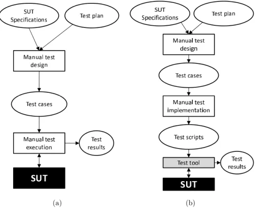
Figure 1.2: Manual (a), and script based (b) test design
Figure 1.2(a) shows the steps of manual testing as the earliest form of confor-mance testing. When manually generating test cases, the test designer uses the specifications of the SUT as an input, and a test plan, which includes the pur-poses/goals of the test. Based on these inputs, the test designer designs the test cases manually, on a high level of abstraction. The so created test cases, are then passed from the test designer to the test engineer. Following the steps described in the test cases, the test engineer executes the test manually, by interacting with the SUT, and recording the outputs that the SUT returns for different inputs. In this stage thus, both the design and the execution of tests were fully manual.
Figure 1.3: Model-based test design
The so-called script based tests make the process of testing easier by automating the test execution phase. As can be seen in Figure 1.2(b) in this case, the test designer does the same job as in the previous case that is, designs the necessary test cases based on system requirements and the test plan. The test engineer on the other hand, rather than manually executing the test based on the high-level test cases, implements a test script. The so created test script then interacts with the SUT that is, it sends different inputs to the SUT, and observes the outputs returned by the SUT. Based on these observations, the script generates a test verdict as its output.
Although script based testing makes test execution a lot easier than in the case of fully manual testing, it is unable to solve the problems raised by manual test design. Thus, tests remain unstructured, their coverage is incomplete, the number of necessary test cases can be huge and thus, they are hard to maintain. In other words, the test is designed in an ad-hoc way, the quality of the test depends on the expertise of the test designer, and the design and maintenance of test cases is time consuming, and costly.
The above mentioned problems of manual test design can be solved by using model-based testingmethods. In the case of model-based testing (Figure 1.3), instead
of manually designing test cases, the test designer has to define the formal model of the SUT on an abstract level [3]. From this abstract model, the model-based testing tool first generates abstract test cases. Then, by concretizing the abstract test cases, the tool generates executable test cases, which can be executed against the SUT [4].
The most widely used models for the formal description of the SUT in model-based testing, are the different finite state machine-model-based models. These are summa-rized by Lee et al. [5], and Dorofeeva et al. [6]. Another formal description technique that can be also used for defining the functional behavior of a communicating sys-tem, is the labeled transition system [7].
Based on the different finite state machine models, many methods have been developed for testing the conformance of a communicating system (i.e. for testing whether the SUT corresponds to a finite state machine). [8–14] present the basic for-mal methods for conformance test derivation, while [15] compares the performance of four of these methods. Lee et al. [16] investigate the existence and identification of distinguishing sequences of finite state machines, which are used for identifying the current state of the SUT. Pap et al. [17], and Brinksma et al. [18] propose test gen-eration and test selection methods. Nemeth et al. [19], and Fakih et al. [20] propose incremental methods for maintaining the test set of a changing conformance specifi-cation. Ghedamsi et al. [21, 22], and Celikkan et al. [23] present methods capable of generating diagnostic tests, which, beyond identifying that the SUT does not corre-spond to its conformance specifications, are capable of localizing the fault. Finally, Tretmans [24] studies conformance testing based on labeled transition systems.
Based on the huge amount of test generation methods, many model-based testing tools have been developed throughout the years, for example Lutess [25], Lurette [26], GATeL [27], TVEDA [28], and AutoLink [29], but the three most widely used tools are Elvior TestCast Generator, [30], Spec Explorer [31], and Conformiq Tool Suite [32].
1.2
Problems of Performance Testing
As we have seen in the previous section, conformance testing has taken a long journey from conformance modeling through test derivation methods, to widely used testing tools. Performance testing on the other hand, has not reached the same level of automation and its methodologies are far from being as much evolved as those of
conformance testing, although performance testing is widely used in the industry. A performance test measures different performance characteristics of the SUT, and is executed against the SUT once it has been found to correspond to its conformance requirements. Some types of performance tests have been classified under different names. Load testing examines how the SUT behaves when increasing the number of requests sent to it. The goal of stress testing is to find the breaking point of the system, i.e. the load under which the system breaks. Finally, scalability testing examines how the system behaves under high loads of data sent to it. Currently, black-box performance tests are designed and executed as shown in Figure 1.4.
Figure 1.4: Performance testing
Thus, black-box performance tests are designed manually, in an ad-hoc way nowadays, without any theoretical background. As the figure shows, based on the performance specifications, the test designer creates and executes the performance test relying on their expertise in the field of performance testing. The test then returns some numerical results that a test engineer has to evaluate and based on which he or she has to decide whether the SUT has passed the performance test or not.
Besides the lack of rigorousness, another problem of performance testing is how to exploit the capacities of the test environment:
During a performance test, the test environment has to generate a relatively high load towards the SUT. The test environment however, is built from universal hardware unlike the SUT, which is built and thus, optimized for a specific purpose.
The reason for this is that the test environment should be able to be reused for different performance tests, which test systems, each of which might be optimized for different purposes. In the industry thus, load generating software entities are used for generating stress towards the SUT. Moreover, for stressing the SUT, multiple hosts are used in the test environment, which are somehow assigned and then execute these load generator entities. This situation demands methods for assigning load generator entities to the hosts of the test environment closely to optimal, in order to exploit the capacities of the test environment as much as possible.
In this thesis, I propose methods for solving the above described two problems of performance testing.
Based on the above open problems of performance testing, my research objectives were
• to define efficient load distribution methods for assigning the load generating software entities to the hosts of the test environment,
• to define a model-driven performance testing method, which outperforms the ad-hoc methods currently used in the industry, and
• to create methods for efficiently improving the performance of the SUT after it has failed the performance test.
Accordingly, the rest of the thesis is organized as follows:
In Chapter 2, I propose load distribution methods for distributing load generator entites among the hosts of the test environment. These methods aim at exploiting the capacities of testing hosts as much as possible.
In Chapter 3, I deal with the theory of performance testing, more specifically, with the subproblem, where the performance requirement of the SUT is the maximal number of request messages that it has to be able to serve within a second while serving a given number of users simultaneously. In this chapter, I propose a model-driven performance testing method, which automatically determines whether the SUT fulfills this performance requirement.
In Chapter 4, I propose methods for correcting the performance of the SUT after it has failed a performance test, which is executed according to the method described in Chapter 3. The presented methods aim at determining how to improve the number of request messages the SUT is able to serve within a second, at minimal cost.
Chapter 2
Load Distribution in a
Performance Testing Environment
As I have mentioned in Chapter 1, the SUT is built for a specific purpose, and its performance is optimized for serving this specific purpose, while the hosts used in the performance test environment (testing hosts from now on) are usually universal hosts, which are used for testing the performance of multiple kinds of SUTs. During a performance test, the test environment has to generate a relatively high load towards the SUT, for a relatively long time. As I have also mentioned, this is achieved by using multiple testing hosts (THs from now on) in the test environment which, together are capable of generating this load (see Figure 2.1).Figure 2.1: Assigning THs to VHs
The load generators or virtual hosts (VHs from now on) used for generating stress towards the SUT, run on THs and usually, the number of VHs is larger than the
number of THs. Each TH has a total capacity, while each VH has a required capacity, and a VH can only be assigned to a TH if, for the whole duration of execution of the VH, the free capacity of the TH is greater than or equal to the required capacity of the VH. Each VH has to be either assigned to a TH or dropped. This assignment has to be carried out by a test controller entity. The objective of the test controller during VH assignment is to maximize the average utilization of THs (that is, to maximize the load generated by the test environment). In the rest of this chapter, I will have the assumption that the total capacity needed to generate the load that the SUT has to be stressed by (that is, the total VH capacity to be assigned) is between TC −δ and TC +δ at all times, where TC is the aggregated capacity of THs, and δ is constant. Beyond its required capacity, for each VH, its starting time and execution time is defined.
The rest of this chapter goes as follows: In Section 2.1, I review the related work in the subject. In Section 2.2, I formally define the load distribution problem, and prove its NP-completeness. In Section 2.3, I formulate the load distribution problem as a binary linear program and propose a solution for solving the problem as a series of binary linear programs. In Section 2.4, I propose a heuristic solution for the load distribution problem. I close the chapter by simulation results comparing the efficiency of the two proposed methods and that of a greedy algorithm in Section 2.5 and by the conclusions of the chapter in Section 2.6.
2.1
Related Work
The problem described above (the load distribution problem from now on) is very similar to the task assignment problem, in which tasks have to be assigned to proces-sors [33]. For the different variants of the task assignment problem, many solutions have been published. [34] presents a family of heuristic algorithms for an extended task assignment problem, in which incompatible tasks can be modelled. [35] presents a solution according to which all the tasks are assigned to clusters the number of which equals the number of processors. After creating the clusters, each cluster is assigned to a processor. [36] introduces a heuristic algorithm for minimizing com-munication costs. The objective of the two algorithms presented in [37] is also to minimize communication costs between tasks. On the other hand, the method in [38] tries to minimize the total amount of time needed to execute all the tasks by using bin packing techniques. [39] proposes the formulation of and two heuristic algorithms
for a special case of the task assignment problem in which, each processor is con-strained in the number of tasks it can handle. [40] uses particle swarm optimization for task assignment. [41] proposes a graph matching based method finding the op-timal solution of the task assignment problem. The methods presented in [42] also finda the optimal solution. One of them works by reducing the search space while the other one executes the task assignment algorithm in parallel to save running time. Finally, [43] proposes a method by which, the efficiency of already existing task assignment heuristics can be improved.
Unfortunately, non of the above solutions are applicable for solving the load distribution problem, since despite its similarity, the load distribution problem differs from the task assignment problem at multiple points: First, the objective of the assignment is different in the two cases; unlike the task assignment problem, in the case of the load distribution problem, there is no need to optimize the solutions for minimizing communication costs and deal with processor connectivity issues. Second, in the case of the load distribution problem, each test component has a predefined starting time, while in the task assignment problem, the starting time of tasks can be arbitrary. As a result of the above, my goal was to develop solutions for the task assignment problem, which will be presented in this section.
2.2
Problem Definition and Complexity
The load distribution problem is defined on a discrete time axis composed of atomic time slots. The problem is defined as follows:
Given are the set of THs T H={THi} and the set of VHsVH={VHi}. Each
TH has one attribute THi = (TCi), where TCi is the total capacity ofTHi. Each
VH has three attributes VHi = (STi,RTi, Ci), where STi is the starting time of
VHi (i.e. the number of the time slot in which VHi starts), RTi is the execution
time ofVHi (i.e. the number of time slots that the execution ofVHi takes), and Ci
is the required capacity of VHi.
The problem to be solved is as follows: For each VHi ∈ VH, choose the value
of assignment function σ ∈ VH → T H from domain D = T HS
{Ø} such that, Formulas 2.1 and 2.2 are true. Choosing THj as the value of σ(VHi) corresponds
to assigning VHi to THj, while choosing Ø as the value of σ(VHi) corresponds to
dropping VHi. In Formula 2.1, U is a lower limit for the total TH capacity. If u is the total TH utilization (used TH capacity to total TH capacity ratio), then
U = u
|T H|
P
i=1
TCitmax. In the formula and the rest of the chapter, tmax denotes the
last time slot (tmax = max
k:VHk∈VH(STk+RTk−1)). |T H| X i=1 tmax X j=1 X k:σ(VHk)=THi∧ ∧STk≤j∧ ∧j≤STk+RTk−1 Ck ≥U (2.1) ∀(i:THi ∈ T H) :∀(j = 1, . . . , tmax) : X k:σ(VHk)=THi∧ ∧STk≤j∧ ∧j≤STk+RTk−1 Ck≤TCi (2.2)
Formula 2.1 states that the total utilization of THs should be above the lower limit U, while Formula 2.2 expresses that for each THi, in each time slot, the
aggregated capacity of VHs running on THi, must be lower than or equal to the
total capacity of THi.
In the following, I prove the NP-completeness of the above defined problem by reducing an arbitrary instance of the NP-complete knapsack problem with equal value and weight functions. During the proof, I first show that the problem is in NP by showing that it can be decided in polynomial time whether an arbitrary solution candidate is a solution (a witness) of the load distribution problem or not. After showing that the problem is in NP, I am going to prove its NP-completeness by defin-ing a mappdefin-ing that transforms an arbitrary instance of the NP-complete variant of the knapsack problem to an instance of the load distribution problem in polynomial time, and by proving that the so obtained instance of the load distribution problem is solvable exactly if the corresponding instance of the knapsack problem is solvable. The main idea of the proof is that the special case of the load distribution problem in which there is only a single time slot, and each VH starts and ends in that time slot, is identical to the NP-complete variant of knapsack problem, in which the cost and the weight of each element are equal to each other. Thus, in this variant of the knapsack problem, there is a single value (x) assigned to each element and packing the elements in the knapsack corresponds to selecting a set of elements for which, the sum of the xvalues is greater than or equal to a lower bound and lower than or equal to an upper bound.
Proof: An assignment defining the value of σ(VHi) for each VH ∈ VH is an
appropriate witness, since the fulfillment of Formulas 2.1 and 2.2 can be verified in O(|VH|+|T H|) time that is, in linear time. This means that the load distribution
problem is in NP. Now, we have to prove that an arbitrary instance of the knapsack problem with equal value and weight functions can be transformed to an instance of the load distribution problem in polynomial time.
The knapsack problem is defined as follows:
Given are a setG, for all of its elements gj a positive integerv(gj) and a positive integer w(gj) and positive integers V and W. The question to be answered is as follows: Is there a subset G′ ⊆G such that the following inequalities are true?
X gj∈G′ w(gj)≤W (2.3) X gj∈G′ v(gj)≥V (2.4)
The knapsack problem remains NP-complete ifv(gj) =w(gj) that is, if the value and weight functions of elements are identical [44]. Thus, let us rename functions w
and v tox. From the so obtained instance of the knapsack problem, an instance of the load distribution problem can be created using the following assignments:
U := V tmax := 1 T H := {TH1} TC1 := W VH := {VHi|gi ∈G} ∀(i:VHi ∈ VH) :STi := 1 ∀(i:VHi∈ VH) :RTi := 1 ∀(i:VHi ∈ VH) :Ci := x(gi) ∀(i:VHi ∈ VH) :σ(VHi) =TH1 ⇔ gi ∈G′ ∀(i:VHi ∈ VH) :σ(VHi) = Ø ⇔ gi ∈/ G′
According to the above assignments, there will be a single TH the total capacity of which equals the capacity of the knapsack. Each element of the knapsack problem corresponds to a VH in the load distribution problem with its weight and value being equal to the capacity of the corresponding VH. The above created instance of the load distribution problem is one dimensional that is, each VH runs in the only time slot, which is time slot 1. The lower limit of total TH utilization U equalsV, which is the lower value limit in the knapsack problem.
Using the above assignments, Formula 2.3 takes the following form:
X
σ(VHi)=T H1
Ci ≤TC1 (2.5)
Using the assignments, Formula 2.4 takes the following form:
X
σ(VHi)=T H1
Ci ≥U (2.6)
Since the above created instance of the load distribution problem has a single TH and a single time slot, and all the VHs run in this single time slot (i.e. for time slot 1, STk ≤ j ∧j ≤ STk+RTk −1 is true for each i : VHi ∈ VH), Formula
2.2 is identical to Formula 2.5 and Formula 2.1 is identical to Formula 2.6, in the case of this instance of the load distribution problem. Thus, Formula 2.3 can be transformed to Formula 2.1 and Formula 2.4 can be transformed to Formula 2.2. The reduction can be carried out in O(|G|) time that is, in linear time. This means that the knapsack problem with equal value and weight functions is Karp reducible to the load distribution problem.
And finally, since the knapsack problem with equal value and weight functions is Karp reducible to the load distribution problem in linear time, and the load distribution problem is in NP, the load distribution problem is NP-complete.
Note: The load distribution problem is a special case of a problem, which is similar to the two-dimensional bin packing problem and only differs from it in its objective function [45]. Thus, the two-dimensional bin packing problem might be a good candidate for proving the NP-hardness of the load distribution problem.
2.3
An ILP Based Heuristic Solution for the Load
Distribution Problem
According to the previous section, the load distribution problem is NP-complete. An effective way to find the optimal solution of an NP-complete problem is formulating it as an integer linear program (ILP), and then solving this ILP.
In the case of the load distribution problem, the ILP is a binary linear program (BLP) meaning that each variable the value of which has to be found can only take
0 or 1 as its value. Before formulating the load distribution problem as a BLP, the boolean variable akj has to be defined (for easier readability) as follows:
akj = 0 ifSTk≤j ∧STk+RTk−1≥ j 1 otherwise (2.7) Furthermore, a new TH TH|T H|+1 has to be introduced. Assigning VHk to
TH|T H|+1 represents dropping VHk. The total capacity of this TH is infinite or
technically, it is equal to the sum of the capacities of all VHs (in order for each VH to be able to be assigned to it), formally:
T H′ =T HS {TH|T H|+1}, where TH|T H|+1 = (TC|T H|+1) and TC|T H|+1 = P k:VHk∈VH Ck (2.8)
After all the above, the BLP formulation of the load distribution problem is as follows. The unknown variables the values of which have to be found are variables
ski. The value of ski is 1 if VHk gets assigned to THi, otherwise its value is 0.
Maximize: |T H| X i=1 tmax X j=1 |VH| X k=1 akjskiCk (2.9) Subject to: ∀(i:THi ∈ T H′) :∀(j = 1,2, . . . , tmax) : |VH| X k=1 akjskiCk ≤TCi (2.10) ∀(k:VHk ∈ VH) : |T H′| X i=1 ski = 1 (2.11) ∀(k :VHk ∈ VH) :∀(i:THi ∈ T H′) :ski ∈ {0,1} (2.12)
The objective function of the problem, Formula 2.9, means that the average utilization of all THs must be maximal that is, the volume of non-dropped VHs must be maximal, where the volume of a VH means the product of its capacity and execution time. THT H+1 is not taken into consideration by the objective function,
to maximize the average utilization of the THs included in set T H.
Formula 2.10 is a constraint stating for each THi ∈ T H that in each time slot,
the aggregated capacity of all the VHs running on THi is lower than or equal to the
total capacity of THi.
Formulas 2.11 and 2.12 define constraints for theski values expressing that from among the ski variables belonging to VHk, exactly one equals 1, while the others
equal 0. Thus, each VH is assigned to exactly one TH included in set T H.
In the above formulation, the number of inequalities that Formula 2.10 produces is |T H|tmin. This number of inequalities is unnecessarily large, since Formula 2.10
can be only violated in the time slots of VH assignment that is, only in those time slots j for which, ∃(i:THi ∈ T H) :STi =j. Thus, it is enough to define Formula
2.10 for those time slots, in which a VH starts. Taking this into consideration, For-mulas 2.13 to 2.16 give an equivalent formulation of the load distribution problem, which omits the unnecessary inequalities produced by Formula 2.10.
Maximize: |T H| X i=1 tmax X j=1 |VH| X k=1 akjskiCk (2.13) Subject to: ∀(i:THi ∈ T H′) :∀(l :VHl∈ VH) : |VH| X k=1 akSTlskiCk ≤TCi (2.14) ∀(k:VHk ∈ VH) : |T H′| X i=1 ski = 1 (2.15) ∀(k :VHk ∈ VH) :∀(i:THi ∈ T H′) :ski ∈ {0,1} (2.16)
The number of equations and inequalities that the above formulation produces is lower than the number of equations and inequalities of the first formulation of the problem (if |VH| < tmax). However, as the later presented simulation results
show, the time needed to solve the BLP formulated by Formulas 2.13 to 2.16 can be extremely large and technically, the BLP cannot be solved in most of the scenarios. The above issue can be solved as follows: First, the time axis should be divided up into time windows, which consist of a given number of time slots. The number of time slots contained in a time window is called the window size, and will be
denoted by W, from now on. Then, starting from the first time window, a BLP is formulated and solved for each time window. The BLP formulated for time window
n defines the assignment constraints of those VHs which start in time window n. The formulation of this BLP depends on (some of the) VH assignments made in the earlier time windows. That is, the solution of the BLP formulated for a given time window serves as an input of BLP formulation of (some) further time windows. The reason for this is that the assignment of VHk toTHi reduces the available capacity
of THi not only for the time window in which VHk was assigned to THi, but for
the whole duration of the execution of VHk.
Each BLP formulated for a time window will give an optimal solution for the corresponding time window, but the global solution, which is thus, composed of a series of sub-optimal solutions will not be optimal in general. The time needed to solve a series of BLPs however, can be reasonable in some scenarios (even though the sub-problems are NP-complete as well).
Formulas 2.17 to 2.20 formulate the load distribution problem for time window
n, with window sizeW. Similarly to Formula 2.14, Formula 2.18 requires the aggre-gated capacity of VHs currently running on each TH to be lower than or equal to the total capacity of the corresponding TH. This constraint is only defined for those time windows in which, a VH starts. In the formulation below, the value of Sk is a reference to the TH to which, VHk was assigned before time window n. That is, Sk =i, if and only ifVHk was assigned toTHi before time windown. IfVHkstarts
after the time window preceding time window n, then Sk = −1. This means that the VH assignments made in earlier time windows serve as an input of formulating the BLP for the current time window. If Sk =|T H|+ 1, then VHk is dropped.
Maximize: |T H| X i=1 nW X j=(n−1)W+1 X k:VHk∈VH∧ ∧STk≥(n−1)W+1∧ ∧STk≤nW akjskiCk (2.17) Subject to: ∀(i:THi ∈ T H′) : ∀(l :VHl∈ VH ∧STl ≥(n−1)W + 1∧STl≤nW) : P k:VHk∈VH∧ ∧STk≥(n−1)W+1∧ ∧STk≤nW akSTlskiCk≤TCi− P k:VHk∈VH∧ ∧Sk=i akSTlCk (2.18)
∀(k :VHk∈ VH ∧STk≥(n−1)W + 1∧STk ≤nW) : |T H′| X i=1 ski = 1 (2.19) ∀(k:VHk ∈ VH ∧STk ≥(n−1)W + 1∧STk ≤nW) : ∀(i:THi ∈ T H′) :ski ∈ {0,1} (2.20) For the whole duration of the test, the VH assignment is carried out by Algorithm 1, which uses the above BLP formulation. The BLP defined by Formulas 2.17 to 2.20 for time window n, is denoted by BLPn in the algorithm.
Algorithm 1 gets sets T H and VH as its input, and outputs the Sk values belonging to each VH.
Algorithm 1: ILP based solution of the load distribution problem
input : T H,VH, W output: S k:VHk∈VH {Sk} 1 foreach VHk∈ VH do 2 Sk:=−1; 3 n:= 1; 4 while (n−1)W + 1≤tmax do 5 Formulate and solve BLPn;
6 foreach k:VHk ∈ VH ∧STk ≥(n−1)W + 1∧STk ≤nW do
7 foreach i:THi ∈ T H do
8 if ski = 1 then
9 Sk :=i
In lines 1 and 2, the algorithm initializes each Sk to initial value -1. From line 4, the algorithm runs iterations, one for each time window. Within an iteration, in line 5, the algorithm formulates and solves the BLP for the current time window. In lines 6 to 9, based on the calculated ski values of the BLP, the algorithm assigns the Sk value of each of those VHs, which were assigned to a TH (or dropped) in the current time window. By the end of the algorithm, each Sk value is known.
2.4
A Bin Packing Based Heuristic Solution for
the Load Distribution Problem
As we will see in the Section 2.5, there are many scenarios in which, the ILP based solution of the load distribution problem cannot be used due to its huge running time, even with a small window size. Thus, I have created a heuristic algorithm for solving the problem. The main idea of the heuristic algorithm is as follows:
When assigning VHk to a TH, other VHs which are assigned and executed
relatively closely in time to VHk have an effect on which THs VHk can be assigned
to, since these VHs occupy TH capacity for their whole execution time, which can be overlapping with the execution time of VHk. Thus, when trying to assign VHs
executed closely in time to each other, without the aggregated capacity of VHs running on a TH at a given point in time exceeding the total capacity of the TH, we have to solve a problem, which is similar to the bin packing problem, where the items packed into bins must fit into the bins and where the assignability of a specific item is affected by the assignments of the other items [46].
Based on the above, we can suspect that applying bin packing heuristics for assigning VHs executed relatively closely to each other, we can achieve a higher average utilization than the average utilization achieved by the greedy algorithm, which always assigns the VH with the next lowest starting time to the first TH that has enough free capacity for the whole duration of the execution of the VH under assignment. In order to be able to assign VHs executed relatively closely in time to each other, the presented heuristic algorithm divides up the [1, . . . , tmax] interval into
time windows of size W, and considers the load distribution problem to be a series of bin packing-like problems, one for each time window, each of which is then solved using a heuristic algorithm similar to the first fit descending (FFD) algorithm [47]. According to the above, the presented heuristic algorithm uses time windows, just like the ILP based solution, but for different reasons. While in the case of the ILP based solution, the goal of using time windows was to reduce the time needed to solve the load distribution problem, in the case of the heuristic algorithm, the goal was to be able to regard the problem as a series of bin packing-like problems.
Algorithm 2 shows the steps of the heuristic algorithm used for solving the load distribution problem. If in the algorithm, Sk equals |T H|+ 1 thenVHk is dropped.
Algorithm 2: Heuristic solution for the load distribution problem input : T H,VH, W output: S k:VHk∈VH {Sk} 1 foreach VHk∈ VH do 2 Sk:=−1; 3 n:= 1; 4 while (n−1)W + 1≤tmax do 5 VHn:={VHk|VHk ∈ VH ∧STk ≥(n−1)W+ 1∧STk≤nW}; 6 VHn←sort VHn by Ck descending; Returnk;
7 k := 1; 8 while k ≤ |VHn| do 9 i:= 1; 10 while i≤ |T H| do 11 if ∀(j :a(VH n[k])j = 1) :CVHn[k]≤TCi− P l:VHl∈VH ∧Sl=i aljCl then 12 SVH n[k]=i; 13 break; 14 i:=i+ 1; 15 if Sk =−1 then 16 Sk :=|T H|+ 1; 17 k :=k+ 1; 18 n:=n+ 1;
Just like the ILP based solution, Algorithm 2 getsT H,VH, andW as its input, and returns the Sk values.
After initializing each Sk to -1 in lines 1 and 2, the heuristics runs iterations, one for each time window. In line 5, the algorithm creates set VHnfrom those VHs,
which start in the current time frame. Then, from line 6 to 17 the heuristics assigns each VH from VHn to a TH in TH′, using a heuristic algorithm similar to the first
fit descending algorithm, according to the following:
In line 6, the elements of VHn are sorted by capacity in descending order and
their references are put into vector VHn. Then for each VHk for which, k is an
element of VHn, starting from the VHk element with the largest capacity, the
VHk that is, the first TH the free capacity of which is greater than or equal to the
capacity of VHk in each time slot in which VHk is running. If the algorithm fails
to find such a TH, then VHk is assigned to TH|T H|+1 that is, VHk is dropped.
Thus, if we regard time windows as the atoms of VH assignment, the heuristics is greedy, since once it has assigned the VHs starting in a given time window to THs, this assignment cannot be changed in latter time windows, and serves as an input of the assignment problems to be solved in latter time windows. However, as the simulation results will show, using the presented heuristic algorithm, the average utilization obtained by the heuristics can be higher than the utilization obtained by the greedy algorithm.
2.5
Simulation Results
In this section, I present simulation results examining the running time of and the average TH utilization achieved by the greedy VH assignment method mentioned in Section 2.4 and the two methods introduced in Sections 2.3 and 2.4. I have run simulations in multiple scenarios, each of which is described by the following parameters:
• |T H| that is, the number of testing hosts,
• TCavg, which is the average TH capacity (denoted by TC in Figures 2.12,
2.13, and 2.14),
• StepTC for which, TCi = TCavg −
|TH|−1 2 −i
StepTC (denoted by Step in
Figures 2.12, 2.13, and 2.14),
• Cavg, which is the average VH capacity and equals 30 in each simulation
sce-nario, and
• ǫC for which, VH capacities are generated on interval [Cavg −ǫC, Cavg +ǫC],
with uniform distribution (denoted by ǫ in Figures 2.12, 2.13, and 2.14). The five simulation scenarios presented in this section are selected from among the 16 simulation scenarios that I have investigated.
During the simulations, the aggregated capacity of all active VHs was on interval [|T H| ∗TCavg −Cavg −ǫC,|T H| ∗TCavg +Cavg +ǫC], in each time slot. In each
simulation scenario, I measured the average utilization and running time of each method as a function of window sizeW. SinceW is not a parameter of the greedy VH assignment algorithm, the average utilization of the greedy algorithm is represented as a horizontal, dotted line in the following figures, while its average running time is represented by horizontal lines with markers in Figure 2.14.
First, let us examine a simulation scenario in which, the highest average utiliza-tion achieved by the heuristic algorithm is not significantly higher than the average utilization of the greedy algorithm.
In the first scenario,|T H|= 3,TCavg = 60,StepTC = 0, whileǫC = 4 that is, the
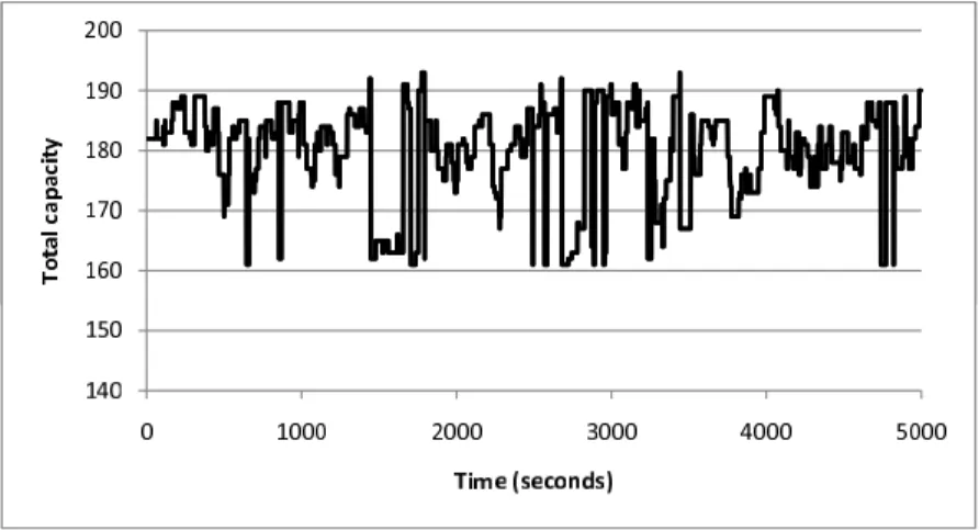
deviation of VH capacities is not large compared to the average VH capacity. Figure 2.2 shows the aggregated capacity of VHs to be assigned to THs in this scenario, as a function of time. The average of this aggregated capacity is the aggregated capacity of all THs.
Figure 2.2: Required capacity, |T H|= 3, TCavg = 60, StepTC = 0, ǫC = 4
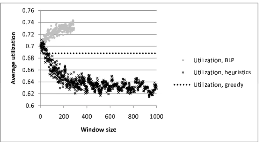
Figure 2.3 shows the average utilization achieved by the three methods. As can be seen in the figure, the average utilization achieved by the ILP based algorithm is higher than the average utilization of the greedy algorithm for each window size and it gets higher the bigger the window size gets. The maximal average utilization achieved by the heuristic algorithm is not significantly higher at its maximum, than the average utilization achieved by the greedy algorithm, in this case. The heuristic algorithm can increase the average utilization of THs by only 3 percent, while the ILP based algorithm can increase the average TH utilization of the greedy algorithm by 8 percent, in this scenario.
Figure 2.3: Average utilization, |T H|= 3, TCavg = 60, StepTC = 0, ǫC = 4
From the results of the first scenario, we can see that if the deviation of VH capacities is small compared to the average VH capacity, the heuristic algorithm does not perform well. This is confirmed by some other simulation scenarios as well, which gave similar results and which are not presented in this section.
In the second scenario, let us see how the proposed methods perform if the deviation of VH capacities is increased. In this scenario, |T H| = 3, TCavg = 60,
StepTC = 0, and ǫC = 20.
Figure 2.4 shows the aggregated capacity of active VHs as a function of time in the second scenario, the average of which, equals the aggregated TH capacity.
Figure 2.4: Required capacity, |T H|= 3, TCavg = 60, StepTC = 0, ǫC = 20
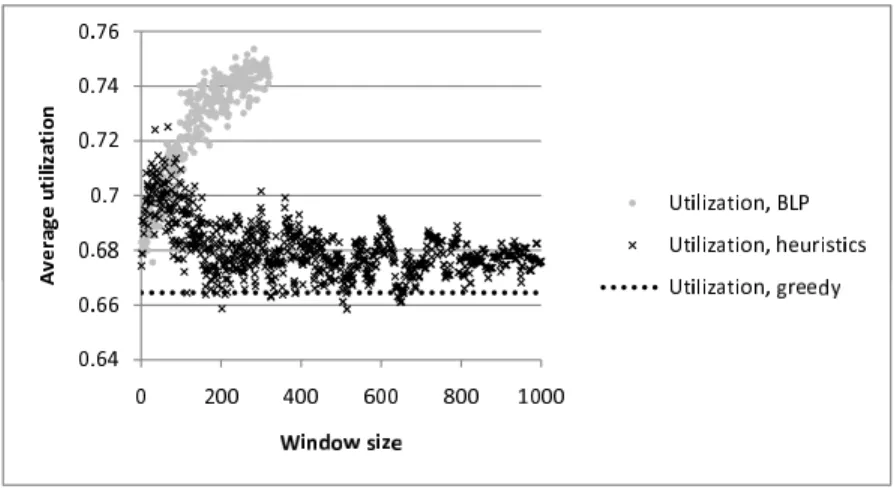
Figure 2.5 shows the average utilization achieved by each method. As it can be seen in the figure, the utilization of the ILP based method gets larger as the window size is increased. The figure also shows that the average utilization achieved by the heuristic method is higher than the average utilization of the greedy algorithm for
almost every window size. In this scenario, the heuristic method performs better than in the first scenario, since the maximal average utilization it can achieve is by 9 percent higher than the average utilization of the greedy algorithm. The ILP based algorithm performs better as well. The highest average utilization it achieves is by 13 percent higher than the average utilization of the greedy algorithm.
Figure 2.5: Average utilization, |T H|= 3, TCavg = 60, StepTC = 0, ǫC = 20
As the results of the second scenario (and other non-presented scenarios) have shown, as the deviation of VH capacities is increased, both the heuristic and the ILP based algorithms perform better.
Figure 2.6: Required capacity, |T H|= 3, TCavg = 210, StepTC = 0, ǫC = 20
In the third scenario, I have investigated, what happens to the performance of the algorithms if the quotient of the average TH capacity and the average VH capacity is higher than in the second scenario. In this scenario, |T H| = 3, TCavg = 210,
applied due to its huge running time, even for small window sizes. Figure 2.6 shows the aggregated capacity of active VHs in each time slot, in this scenario. The aggregated VH capacity equals the aggregated TH capacity, in average.
Figure 2.7 shows the average utilization of the greedy and the heuristic algorithm. According to the figure, the performance of the heuristic method is not significantly higher than that of the greedy algorithm, in this scenario. The maximal average utilization achieved by the heuristic algorithm is only by 2 percent higher than the average utilization achieved by the heuristic algorithm.
Figure 2.7: Average utilization, |T H|= 3, TCavg = 210,StepTC = 0, ǫC = 20
According to the results of the third scenario (and some non-presented scenarios with similar results), the performance of the heuristic algorithm gets worse as the quotient of the average TH capacity and the average VH capacity is increased.
Let us now investigate two scenarios in which, TCavg = 60, and ǫC = 20 that
is, two scenarios in which the quotient of the average TH capacity and the average VH capacity is lower than in the third scenario and the deviation of VH capacities is higher than in the first scenario.
In the fourth scenario, I have changed the parameters of the second scenario so that TH capacities are not uniform. In this scenario |T H| = 3, TCavg = 60,
StepTC = 5, while ǫC = 20. Figure 2.8 shows the aggregated capacity of active VHs as a function of time, in this scenario. Just like in the previous scenarios, the aggregated capacity of active VHs equals the aggregated capacity of THs, in average.
Figure 2.8: Required capacity, |T H|= 3, TCavg = 60, StepTC = 5, ǫC = 20
Figure 2.9 shows the average utilization of each method, in the fourth scenario. According to the figure, the heuristic algorithm produces higher average utilization values for each window size than the greedy algorithm, while the ILP based method gets more efficient as the window size increases.
Figure 2.9: Average utilization, |T H|= 3, TCavg = 60, StepTC = 5, ǫC = 20
According to the results of the fourth scenario, in this case, the algorithms per-form just as well as in the second scenario. The maximal average utilization achieved by the heuristic method is by 10 percent higher than the average utilization of the greedy algorithm, while the average utilization of the ILP based method is by 17 percent higher than that of the greedy algorithm at maximum.
Finally in the fifth scenario, let us see how the performance of the presented methods changes if the number of hosts of the fourth scenario is increased from 3 to 9. Thus in the fifth scenario, |T H| = 9, TCavg = 60, StepTC = 5, and ǫC = 20.
Figure 2.10 shows the aggregated active VH capacity as a function of time, which equals the aggregated TH capacity in average, just like in all the previous cases.
Figure 2.10: Required capacity, |T H|= 9, TCavg = 60, StepTC = 5, ǫC = 20
In this case, just like in the third scenario, the running time of the ILP based algorithm was extremely long even for small window sizes and thus, it could not be executed. Figure 2.11 shows the average TH utilization achieved by the bin packing based heuristic and the greedy methods, with different window sizes.
Figure 2.11 shows that the heuristic algorithm gives a higher average utilization value than the greedy algorithm, for each window size.
Figure 2.11: Average utilization, |T H|= 9, TCavg = 60, StepTC = 5, ǫC = 20
As the results of the fifth simulation scenario have shown, the performance of the heuristic algorithm remains good compared to that of the greedy algorithm if the number of testing hosts is increased. The maximal average utilization achieved by the heuristic algorithm is by 8 percent higher than the average utilization achieved by the greedy algorithm.
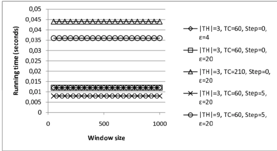
Figure 2.12 shows the running time of the ILP based heuristics on a logarithmic vertical axis, Figure 2.14 shows the running times of the greedy algorithm, while Figure 2.13 shows the running times of the bin packing based heuristics as a function of window size, for the different simulation scenarios. As it can be seen in the figures, both heuristic solutions have reasonable running times. The running time of the ILP based heuristic on the other hand, grows exponentially as the window size increases and as mentioned earlier, in two simulation scenarios it could not be executed at all due to its huge running time. As it can also be observed in the figure, the curves representing the running time of the ILP based solution start with a descent. The reason for this descent is the overhead caused by having to formulate a large number of binary linear programs in the case of lower window sizes.
Figure 2.12: Running times of the ILP based algorithm
Figure 2.14: Running times of the greedy algorithm
Table 2.1 summarizes the above presented results by showing the maximal aver-age utilization values achieved by each method in each scenario.
Scenario Average utilization |T H| TCavg StepTC ǫC BLP Heuristics Greedy
3 60 0 4 0.743811 0.710993 0.688083 3 60 0 20 0.753542 0.725086 0.664499 3 210 0 20 − 0.888547 0.869548 3 60 5 20 0.773141 0.730494 0.663302 9 60 5 20 − 0.78783 0.727412
Table 2.1: Maximal average utilization values achieved by different methods in dif-ferent scenarios
As it can be observed in the figures plotting the average utilization values ob-tained by each method, the values close to the maximal average utilization value are concentrated to a narrow window size interval, in the case of the heuristic al-gorithm, and the average utilization obtained by the heuristic algorithm decreases both if the window size is increased beyond this interval and if it is decreased below this interval. The reason for this is as follows:
If the window size is too small then the heuristic algorithm takes too few VH assignments into consideration at one time and thus, approaches the greedy algo-rithm (which takes a single VH into consideration at one time). If however, the window size is too large, then there might be VHs in the same time window, which are executed far from each other in time. The assignabilities of these VHs are not
affected by each other and thus, the problem of assigning VHs of the same, large time window is not similar to an instance of the bin packing problem anymore. Thus, using bin packing heuristics for large window sizes does not make any sense. As it can also be observed in the above figures, the bigger the window size is, the more effective the ILP based solution gets in means of average utilization. The reason for this is that increasing the window size makes the sub-problem of assigning VHs of the same window size approach the problem of assigning all VHs to THs in which, W =tmax, and for which, the ILP based method finds the optimal solution.
The simulation results have shown that there is always a window size for which, the heuristic algorithm achieves a higher average utilization value than the one achieved by the greedy method. We can furthermore, draw the following conclusions: As the quotient of the average TH capacity and the average VH capacity de-creases or the deviation of VH capacities inde-creases, the average utilization achieved by the proposed methods gets more significantly higher than the average utiliza-tion achieved by the greedy algorithm. The ILP based method can always achieve a higher average utilization than the heuristic method. However, it can only be applied if the quotient of the average TH capacity and the average VH capacity is relatively small and there are a relatively few THs, since this is the only case in which its running time is not unreasonable. The running time of the heuristic method is however, about the same as that of the greedy algorithm, while its maximal average utilization is approximately halfway between the maximal average utilization of the BLP method and the average utilization of the greedy algorithm (even in the cases where it does not perform significantly better than the greedy algorithm). Thus, the heuristic algorithm can be used more effectively than the greedy algorithm in almost any scenario, but it is the only option if the number of THs is big, and the quotient of the average TH capacity and average VH capacity is small. The scenario in which the greedy algorithm might be the best choice is the one in which, the deviation of VH capacities is relatively small and the quotient of the average TH capacity and the average VH capacity is relatively big. The reason for this is the following:
In this case, the ILP based algorithm cannot be used due to its huge running time. The heuristic algorithm on the other hand, does not achieve a maximal av-erage utilization, which is significantly higher than the one achieved by the greedy algorithm. Moreover, while the greedy algorithm needs O(|TH||VH|) steps to fin-ish, a single execution of the heuristic algorithm needs O(|TH||VH|c) steps, where
differ-ence might not be significant in the practice, but the effective running time of the heuristic algorithm can be by orders of magnitude higher than that of the greedy algorithm, since in order to find the maximal average utilization provided by the heuristic algorithm, it has to be executed for multiple window sizes. According to the simulations, the time window size that gives the highest average utilization in the case of the heuristic algorithm, is between 0 and the average VH execution time, which is around 90 in the above scenarios, or it is slightly higher than the average VH execution time.
2.6
Conclusions
The goal of this chapter was to improve the efficiency of test component assignment in performance test environments. The motivation of the chapter was that test components are assigned to the testing hosts of the test environment in a greedy way and thus, I expected that by using more sophisticated methods, the average utilization of testing hosts can be increased. After formulating the load distribution problem, I have investigated methods created for solving the similar task assignment problem and found that because of the differences of the two problems, neither of these solutions are applicable for solving the load distribution problem.
In order to improve the average utilization of testing hosts reached by the greedy method, I have defined different heuristic solutions for solving the problem. After evaluating the efficiency of my heuristics against that of the greedy method, I found that in most of the cases, the heuristics reach a significantly higher average utilization of testing hosts than the greedy algorithm.
Chapter 3
A Model-Driven Performance
Testing Method for
Communicating Systems
As I have mentioned in Chapter 1, unlike conformance testing, the field of black-box performance testing of communicating systems lacks an evolved theoretical back-ground, including automatic methods for checking whether the SUT fulfills its per-formance requirements, for example whether it is able to serve a specified number of request messages within a second while serving a specified number of users in par-allel. Unlike conformance tests, black box performance tests are mainly designed in an ad-hoc way in the industry. The disadvantage of this approach is the inaccuracy of the performance test results meaning that the deviation of ad-hoc performance measurements is larger than necessary, as we will see.
To solve the above described problem of performance testing, in this chapter, I introduce an automatic model-driven performance testing method. The presented method interacts with the SUT, and based on this interaction and on the functional characterics of the SUT, it creates its formal performance model. Based on this performance model, the method determines whether the SUT fulfills the performance requirement of serving the required number of request messages within a second while serving a given number of users.
This chapter is organized as follows: In Section 3.1, I give a summary on the related work in the subject. In Section 3.2, I discuss the performance requirements that I deal with, and the motivations of creating the proposed performance testing
method. In Section 3.3, I formally define my performance model used for testing, then in Section 3.4, I show how to create the structure of the performance model of the SUT. In Section 3.5, by performing measurements on the SUT, I show how to complete the performance model of the SUT. In Subsections 3.5.1 and 3.5.2 I show how to calculate CWusr and CEusr, respectively, based on the performance model
of the SUT. I close the section by experimental results comparing my performance testing method to an ad-hoc performance testing method used in the industry, in Section 3.6 and a summary of the results achieved in Section 3.7.
3.1
Related Work
As I have mentioned in Chapter 1, In the field of conformance testing there are formal methods for automatically checking whether a physical system conforms its specifications. These methods include:
• formal methods for modeling the functional requirements of the SUT, and • methods for checking whether the SUT corresponds to this formal model In the field of performance testing, there exist different solutions for defining performance tests. Schieferdecker et al. have proposed PerfTTCN [55], which ex-tends TTCN-2 (Tree and Tabular Combined Notation ver. 2) [56]. It introduces many new language elements for describing performance testing environments and for conducting performance tests. As a language extension of TTCN-3 (Testing and Test Control Notation ver. 3) [57], Grabowski et al. introduce TimedTTCN-3 [58]. TimedTTCN-3 extends TTCN-3 and makes it capable of testing the real-time be-havior of the SUT. Mingwei et al. extend concurrent TTCN (which is a version of TTCN-2) to be able to test the performance of communication protocols [59, 60].
The performance property I dealt with (the number of messages the system is able to process within a second while serving a given number of users) is however, more complex than the ones the above mentioned methods can measure. For the measurement of this property, ad-hoc methods are used in the industry [61]. Thus, my goal was to create a more efficient model-driven performance testing method during which, a formal performance model of the SUT is created and then the per-formance characterictics to be measured are derived from this perper-formance model.
In the literature, there already existed papers written on performance modeling. In [48], Kemper et al. present a performance model for communicating systems, based on SDL (Specification and Description Language) [49]. Youness et al. [50] use a stochastic Petri net [51] while El-Karaksy et al. use a timed Petri net [52] for modeling the performance of a communication protocol [53]. Marsan et al. model the performance of CSMA/CD bus LANs by a timed Petri net based model [54]. These papers also verifythe models presented, that is, they analytically prove that their models correspond to the specifications, but they do not deal with validating a physical system that is, they do not offer methods for testing whether a physical implementation corresponds to the performance model.
Thus, the solution for the problem was to create a performance model, which could represent a physical system and based on which, a performance testing method could be defined for calculating the number of messages the represented system is able to process within a second while serving a given number of users in parallel.
3.2
Performance Requirements and Motivations
As I have mentioned earlier, the presented method is given as an inputCRusr, which
is the number of messages to be processed within a second while serving usr users (number of messages per second for short). The method evaluates the performance of the SUT automatically, in other words it determines the number of messages the SUT can process within a second while serving usr users simultaneously.
CRusr as a performance requirement is ambiguous. Thus, I interpreted this
notion in two ways. CRusr can be disambiguated as CWRusr, which is the required
number of messages that the SUT has to be able to serve within a second, in worst case while serving usr users. By worst case, I mean that the SUT has to be able to serve CWRusr messages per second given any sequence of requests it receives from
the users. CRusr can also be disambiguated asCERusr, which is the expected number
of messages the SUT has to be able to serve within a second while servingusr users. I am going to state as a requirement of my performance testing method the ability of measuring both CWusr, which is the worst-case number of messages andCEusr,
which is the expected number of messages the SUT is able to serve within a second, while servingusr users simultaneously. The performance testing method introduced in this section attempts to solve the problems raised by the ad-hoc performance testing methods, which are widely applied in the industry nowadays [61].
The ad-hoc performance testing method measures the performance of the tested system in a straightforward way, by simply emulating the real-life environment the SUT will have to operate in. Thus, this method runs a number of software entities, each emulating a user that the SUT has to serve. The number of software entities run by the test environment equals usr. During the test, each emulated user sends one request message after another to the SUT, and counts the number of responses the SUT has sent in reply. At the end of the test, the number of messages the SUT is able to serve within a second is calculated as the quotient of the number of all responses the SUT has sent to the software entities, and the duration of the test. This method can calculate CEusr. However, as we will see during the experiments,
the deviation of the CEusr values measured by this method is larger than necessary.
The ad-hoc method is furthermore, unable to calculate CWusr. Thus based on its
measurements, we can only state that CWusr is lower than or equal to the lowest
CEusr value measured by the ad-hoc method.
Contrarily to the ad-hoc method, the proposed method is capable of calculating both CEusr and CWusr. My method uses a formal performance model as a tool for
conducting the performace test and for modeling the SUT. The proposed method has two phases. In the first phase, from the information already known about the SUT, and from measurements performed on the SUT, the test environment creates the performance model of the SUT. In the second phase, the method derives both CWusr and CEusr from the so created performance model, in an analytical
way. The first phase is discussed in Sections 3.3 and 3.4, while the second phase is discussed in Section 3.5. As we will see during the experiments, my method gives correct measurement results that is, the CEusr value it calculates is theCEusr value
calculated by the ad-hoc method, while the CWusr value it calculates is lower than
each ad-hoc measurement. As we will also see, the deviation of the CEusr values
measured by my method within a given amount of time is smaller than the deviation of theCEusr values measured by the ad-hoc method within the same amount of time.
3.3
The Timed Communicating Finite Multistate
Machine
In this section, I introduce the Timed Communicating Finite Multistate Machine model, which will be used for conducting the performance test. At the end of the
test, this model is a performance model of the SUT. In the definition below, I first give the formal definition of the TCFMM, then give a brief informal description. After that, I explain the non-trivial constraints of the definition one-by-one. In the definition, τ0 denotes the time of the beginning of the execution.
Definition 1 The Timed Communicating Finite Multistate Machine (TCFMM) is
a 10-tuple:
TCFMM = (I, O, S, s0, T, U, H, δ, χ, σ), where
1. T ⊆I×O×S×S×R+
2. ∀ti, tj ∈T((ti = (ii, oi, sfromi, stoi, di)∧tj = (ij, oj, sfromj, stoj, dj)∧
sfromi =sfromj ∧ii =ij)⇒ti =tj) 3. χ∈H →U, χ is bijective 4. s0 ∈S 5. σ∈R+×U →S∪ {⊘} 6. ∀(u∈U) :σ(τ0, u) =s0 7. δ∈R+×H×I →S×O×R+ 8. ∀(ti ∈T, h∈H, τ ∈R+) :σ(τ, χ(h)) =s fromi ⇒δ(τ, h, ii) = (stoi, oi, di)
and invalid inputs are dropped. 9. ∀(τ, h, i, s, o, d:δ(τ, h, i) = (s, o, d)) : (∀(φ: 0< φ < d) :∀(u∈U − {χ(h)}) : P(σ(τ +φ, u) =⊘) = 1 ⇒(σ(τ+d, χ(h)) =s∧ ∀(ǫ: 0< ǫ < d) : σ(τ+ǫ, χ(h)) =⊘))∧(¬(∀(φ : 0< φ < d) :∀(u∈U − {χ(h)}) : P(σ(τ +φ, u) =⊘) = 1)⇒ ∃(d′ :d′ < d) : (σ(τ+d′, χ(h)) =s∧ ∀(ǫ: 0< ǫ < d′) :σ(τ+ǫ, χ(h)) =⊘))∧ ∧∃(ti ∈T) :sfromi =σ(τ, χ(h))∧stoi =s∧ii =i∧oi =o∧di =d
In the definition above, I is the set of inputs, O is the set of outputs of the TCFMM, S is the set of states with s0 being the initial state, and T is the set of
state transitions. H is the set of users communicating with the TCFMM, while U
is the set of tokens in the TCFMM, each one belonging to a user. Finally, σ is the current state function, δis the state transition function, and χis the function which assigns each user to a token.
The TCFMM is an extension of the Finite State Machine model. It has states connected by transitions, just like an FSM. One of my goals was to extend the FSM