and Public Health
Article
A Comparison of Spatio-Temporal Disease Mapping
Approaches Including an Application to Ischaemic
Heart Disease in New South Wales, Australia
Craig Anderson1,2,* and Louise M. Ryan1,2
1 School of Mathematical and Physical Sciences, University of Technology Sydney, 15 Broadway, Ultimo,
NSW 2007, Australia; [email protected]
2 ARC Centre of Excellence for Mathematical and Statistical Frontiers (ACEMS), Parkville, VIC 3010, Australia
* Correspondence: [email protected]; Tel.: +61295148039 Academic Editor: Jamal Jokar Arsanjani
Received: 14 December 2016; Accepted: 20 January 2017; Published: 3 February 2017
Abstract: The field of spatio-temporal modelling has witnessed a recent surge as a result of developments in computational power and increased data collection. These developments allow analysts to model the evolution of health outcomes in both space and time simultaneously. This paper models the trends in ischaemic heart disease (IHD) in New South Wales, Australia over an eight-year period between 2006 and 2013. A number of spatio-temporal models are considered, and we propose a novel method for determining the goodness-of-fit for these models by outlining a spatio-temporal extension of the Moran’s I statistic. We identify an overall decrease in the rates of IHD, but note that the extent of this health improvement varies across the state. In particular, we identified a number of remote areas in the north and west of the state where the risk stayed constant or even increased slightly.
Keywords:spatio-temporal modelling; disease mapping; Bayesian; ischaemic heart disease, Moran’s I
1. Introduction
The field of spatial modelling has grown substantially over the last several decades as advances in geographic information systems (GIS) have facilitated the incorporation of spatially-indexed outcomes and/or covariates within epidemiological and environmental models. Spatial models have a vast
range of applications in areas such as disease mapping [1], air pollution monitoring [2] and ecology [3].
These approaches allow more accurate modelling of the spatial pattern of the outcome of interest by accounting for the underlying spatial autocorrelation structure. It is natural to extend these approaches to identify the changes in these spatial patterns over time, with the aim of identifying either localised
or global trends. Simple spatio-temporal models have existed for over 40 years (e.g., [4]), but recent
developments in both computational power and the gathering and publication of vast amounts of data have led to a recent surge in the spatio-temporal literature.
The key aim of spatio-temporal modelling is to account for the evolution of outcomes in both space
and time simultaneously. Cressie and Wikle [5] provide an excellent introduction to spatio-temporal
modelling and outline some of the standard techniques used in this area. Spatial data takes two key forms—areal (or lattice) data and point-referenced (or geostatistical) data—and a variety of
spatio-temporal models have been developed for each type of data (e.g., [6–9]).
This paper focuses on modelling ischaemic heart disease (IHD) hospital admissions in New South Wales, Australia between 2006 and 2013. IHD is responsible for around 20,000 deaths per year in Australia, and is the most common cause of death for both males and females. IHD risk has decreased substantially over the last three decades, but these decreases are not necessarily uniform across all
regions. We are therefore interested in identifying any localised inequalities that may be present for IHD risk.
The diversity of the applications, data types and conceptual approaches to modelling means that the spatio-temporal modelling literature is somewhat diffuse. Therefore, a further contribution of this paper is to provide an overview of these spatio-temporal modelling approaches in order to identify similarites and differences between these existing approaches and to make recommendations for practice. We also wish to provide a quantitative comparison of the methodologies using some form of spatio-temporal goodness-of-fit test, an area which has received little attention in the literature.
We therefore propose a novel use of a spatio-temporal Moran’s I statistic [10] as a method for measuring
the extent of spatio-temporal autocorrelation in the residual values from the model fits.
The remainder of this paper will be structured as follows: Section 2provides an overview
of spatio-temporal modelling, including a discussion of existing methodology for analysing
spatio-temporal data; Section3describes our IHD dataset and outlines the modelling approaches
which will be carried out in our analysis and Section4displays the results of this analysis. Section5
provides a summary of the paper and recommendations in practice and Section6outlines the key
conclusions of our work.
2. Methodology
The spatial (and spatio-temporal) modelling literature centres around two main data types: areal (or lattice) and point-referenced (or geostatistical). Point-referenced data structures are based on the exact geographical location of an observation being recorded, generally in the form of latitude and longitude co-ordinates. This form of data is commonly used for monitoring environmental outcomes, where spatial modelling approaches can be used to characterise the nature of an environmental outcome across the entire study region based on a finite set of monitoring stations. Areal data structures are based on the study region being partitioned into a set of non-overlapping subregions known as areal units—for example, a county being divided into a set of postcode areas. Areal data are commonly used in health applications, where confidentiality issues prevent the exact geographical locations of disease cases being recorded. Instead, only the patient’s areal unit is recorded, and the data consists of an aggregated count for each individual areal unit. Thus, it is possible to conceptualise areal data as an aggregation of point-level data. Our ischaemic heart disease data is areal, and, therefore, this section will focus on discussing existing methodology for areal data. We will first outline the methodology used in a spatial context, and then show how this can be extended to account for spatio-temporal data.
2.1. Spatial Modelling
The aim of areal modelling is to estimate the occurence rate of an outcome (such as disease risk) in each areal unit, thus providing a set of risk estimates that cover the entire region. We may
also be interested in identifying the spatial extent of covariate effects. Consider a study regionA,
partitioned intonnon-overlapping areal units such thatA= {A1, . . . ,An}. A responseYiis observed in
each areal unit, thus providing a set of response dataY = (Y1, . . . ,Yn). Area-level covariate information
X = (xT1, . . . ,xTn)may also be available. In most cases, it is important to account for differences in
population demographics across the study region, since some subregions are likely to contain a larger at-risk population. For example, areas which have a higher percentage of elderly people are likely to have higher rates of heart disease than those with a younger population, but this does not necessarily mean that there is any underlying in disease risk rate between the regions. We can account for these
demographic differences by constructing a set of expected disease countsE= (E1, . . . ,En), whereEiis
the expected number of disease cases in areai. These expected counts can be constructed using either
internal or external standardisation based on the age and sex demographics of the population within each areal unit.
Based on these expected counts, one simple measure of disease risk is the standardised incidence
ratio (SIR), which is computed for areaias
SIRi=
Yi
Ei. (1)
An SIR value larger than 1 indicates that a region has a higher than expected disease risk, while an SIR less than 1 implies a lower than expected risk. The SIR provides a useful exploratory tool but has the major disadvantage that it considers each areal unit independently and does not account for any form of spatial structure in the data. Additionally, in cases where a rare disease or a small population
is being studied, some areal units may have a very low expected valueEi, and the SIR would be
susceptible to small random fluctuations in the responseYi.
It is therefore more common to use a generalised linear model to estimate disease risk. Models for spatial data are based on an underlying belief that there is some form of correlation between areal units that are close to each other geographically. Given that the response is almost always based on count data, modelling is generally based on a Poisson log-linear model of the following form:
Yi ∼ Poisson(Eiµi) i=1, . . . ,n, (2)
log(µi) = xTiβ+φi.
Here,µirepresents the mean risk for areai,βis the set of coefficients relating to the covariatesX
andφiis a random effect specific to areai, used to account for unexplained spatial autocorrelation.
The set of random effectsφ= (φ1, . . . ,φn)are commonly represented by a conditional autoregressive
(CAR) prior distribution. CAR priors can typically be specified via a multivariate normal distribution
φ∼N(0,Σ), (3)
with a covariance function Σ that reflects the spatial correlation between the random effects.
Besag et al. [11] proposed the intrinsic CAR prior with covariance matrixΣ=τ2(D−W)−1, where
τ2is a conditional variance parameter andDandWare matrices determined by the neighbourhood
structure of the data. D is a diagonal matrix where theith entry on the diagonal is equal to the number
of neighbours for areal uniti.Wis a neighbourhood matrix which is defined as follows:
wii0= (
−1 ifi∼i0,
0, otherwise.
Here,i∼i0means that areasiandi0are neighbours. Typically, areas are defined as neighbours if
they are adjacent and thus share a common border, though other specifications are also possible [12].
This specification does not have a parameter that controls the strength of the spatial correlation,
and is thus inappropriate in cases with weak spatial correlation. The work of Cressie [13] and
Leroux et al. [14] led to a more generalised version of the original that accounted for different strengths
of spatial correlation using an additional smoothing parameterρ. The covariance matrix is redefined as
Σ=τ2(D−ρW)−1, whereρcontrols the level of spatial correlation present, withρ=1 corresponding
exactly to the intrinsic CAR model outlined above, andρ = 0 corresponding to complete spatial
independence. It is generally straightforward to estimateρfrom the data.
An alternative method for handling different strengths of spatial correlation is the
Besag–York–Mollie (BYM) model, proposed by Besag et al. [11]. The BYM model extends the intrinsic
log(µi) =xTi β+φi+θi, (4)
whereθi ∼ N(0,σ2). Different strengths of spatial correlation can be accounted for by varying the
relative sizes of the random effectsφandθ. The main drawback of this approach is that only the sum
φi+θiis identifiable for each region, but, nonetheless, the BYM approach remains popular within the
spatial and spatio-temporal literature.
2.2. Spatio-Temporal Modelling
The spatial models outlined in Section 2.1 apply to data observed at a single time point,
but there are many cases where data from multiple time points are available. In addition to the spatial correlations described in the previous section, these data will also have temporal correlations, with observations at consecutive time points having more in common than those further apart. There is also the possibility of a space–time interaction, given that different areas may have different temporal trends, and these trends may be more similar in areas which are closer together geographically.
Consider the case where data are collected acrossJdiscrete time points at each of thenareal units.
We have response dataY= (Y1, . . . ,Yn)whereYi= (Yi1, . . . ,YiJ)is the set ofJobservations for areai.
We consider the case where the timepoints are the same at each location, though this is not necessary for all models.
The majority of spatio-temporal models for areal data have been developed by extending the
spatial model (2) as follows:
Yij ∼ Poisson(Eijµij) i=1, . . . ,n, j=1, . . . ,J,
log(µij) = xTijβ+si() +uj() +vij(), (5)
wheresi()is a function that captures spatial correlation,uj()is a function for temporal correlation and
vij()is a function capturing space–time interaction. However, while this formulation is conceptually
straightforward, implementation can be difficult, especially with larger datasets. The biggest challenge
in such approaches is making a choice for the spatio-temporal term vij() that accurately reflects
the underlying spatio-temporal risk structure, and, in particular, the possibility of different trends occurring in different regions. The remainder of this section provides an overview of the existing
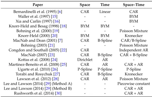
literature for spatio-temporal modelling. Table1provides a brief summary of the literature covered
in this section, and, in particular, the types of spatial, temporal and spatio-temporal effects used in each method.
One of the earliest spatio-temporal models for areal data was proposed by Bernardinelli et al. [6],
who suggested a model where each areal unit has a separate linear trend. Here,si() =φi, a spatial
random effect,uj() =βtj, a linear trend over time andvij() =ηitj, the area-specific deviation from
the trend. Bothφandη are modelled by a CAR prior, as outlined in Section2.1. This approach
therefore allows each areal unit to have its own intercept modelled byφiand its own slope modelled
by(β+ηi)tj. Although this approach is flexible in allowing each areal unit to have its own trend, it is
restrictive in requiring these trends to be linear, which may not be appropriate in many applications.
An alternative approach was outlined by Waller et al. [15], who proposed a spatio-temporal
extension of the BYM model (4). The authors propose fitting a separate BYM model at each time point,
which issi(),uj() =0 andvij() =θi(j)+φi(j), whereφ(j)is a set of random effects at timejmodelled by
a CAR prior, andθ(j)is a set of independent random effects. This formulation allows a different spatial
pattern to be estimated at each time point, with the patterns being uncorrelated from one time point to
the next. A similar approach is outlined by Xia and Carlin [16], who also include an age-group specific
term to allow different trends for different age groups. However, these approaches make no attempt at smoothing over time, which may not be realistic in practice. One would expect some sort of temporal correlation to exist in most spatio-temporal datasets, and models should ideally account for this.
Table 1.Summary of the structures of the spatio-temporal models discussed in this paper. The following abbreviations are used in the table: AR = autoregressive model [17], BYM = Besag–York–Mollie model (4), CAR = conditional autoregressive model (3).
Paper Space Time Space–Time
Bernardinelli et al. (1995) [6] CAR Linear CAR
Waller et al. (1997) [15] - - BYM
Xia and Carlin (1997) [16] - - BYM
Knorr-Held and Besag (1998) [18] BYM BYM -Bohning et al. (2000) [19] - - Poisson Mixture
Knorr-Held (2000) [20] BYM BYM Kronecker MacNab and Dean (2001) [7] CAR B-Spline CAR/B-Spline
Bohning (2003) [21] - - Poisson Mixture
Congdon and Southall (2005) [22] CAR Independent AR MacNab (2007) [23] CAR B-Spline CAR + B-Spline Kottas et al. (2008) [24] Dirichlet AR -Martinez-Beneito et al. (2008) [25] CAR AR CAR + AR
Ugarte et al. (2010) [26] P-Spline P-Spline P-Spline Torabi and Rosychuk [27] CAR B-Spline Kronecker
Lawson et al. (2012) [28] CAR AR Poisson Mixture Lee and Lawson (2014) [29] (Method A) - - Piecewise constant Lee and Lawson (2014) [29] (Method B) - - CAR + AR
Rushworth et al. (2014) [30] - - CAR + AR
An alternative temporal extension of the BYM model is proposed by Knorr-Held and Besag [18].
They propose a model consisting of a pair of spatial random effects and a pair of temporal effects, with
each pair consisting of one structured term and one unstructured term. This model hassi() =φi+θi,
uj() =αj+γjandvij() =0, whereφis modelled by a CAR prior,αfollows a first order random walk
in time and (θ,γ) represent independent random effects with mean 0 and variancee. The authors
acknowledge that their model combines space and time additively and does not make provisions for cases where there is an interaction between time and space.
Knorr-Held [20] addresses this problem by extending [18] to include an additive space–time
interaction termvij() =δij. This interaction term has a covariance structure specified by the Kronecker
product of the structures of the random effects which are interacting. Of particular interest is the case
where the spatially correlated random effectφand the temporally correlated random effectαinteract.
In this case, the spatio-temporal random effectδhas a specification that combines a spatial CAR model
and a random walk in time. These approaches are thus able to account for spatial and temporal trends as well as potential area-specific differences in trends, but, over longer time periods, the random walk may not capture the complexity of the temporal trends.
Non-parametric smoothing approaches provide an alternative way to capture temporal trends in
spatio-temporal models. One of the first such approaches was proposed by MacNab and Dean [7],
who outlined a generalised additive mixed model for estimating disease risk, combining a CAR
model for the spatial pattern (si() =φi) and a set of smooth functions known as B-splines [31] for the
temporal trends. The authors discuss two possible formulations for the space–time interaction term:
one parametric and one non-parametric. The parametric approach follows [6] by allowing spatially
correlated area-specific linear deviations from the global trend by settingvij() =ηitj, whereηfollows
a CAR prior. The non-parametric approach models the spatio-temporal termvij()using area-specific
B-splines for each region, thus allowing nonlinear area-specific deviations. The interaction term is spatially correlated in the parametric approach, but not in the non-parametric approach, where the area-specific deviations are assumed to be independent. However, the non-parametric approach allows a great deal more flexibility and may therefore provide a more realistic estimation of temporal trends, particularly in applications covering longer time periods.
MacNab and Gustafson [32] proposed a method that combined both of these appealing properties by including spatially-varying B-splines that allow the interaction term to be nonlinear but still spatially correlated. This is achieved by allowing the set of coefficients of the area-specific B-splines to follow a CAR prior, thus inducing correlation in the spline coefficients between areas which are close together. An alternative approach to modelling the space–time interaction in this model form
was proposed by Torabi and Rosychuk [27], who proposed a covariance structure similar to that used
in the fully-parametric form in [20]. Here,vij()is modelled with a covariance matrix given by the
Kronecker product of the spatial random effects and the B-splines. These approaches are all based on using B-splines for smoothing, but more flexible smoothing approaches are available, and these could be more appropriate in certain applications.
MacNab [23] compared the B-spline smoothing approach to a number of specifications which
used either smoothing splines [33] or P-splines [34]. For the B-spline model, the author had to run
multiple models, each with a different number of knots, in order to select the optimal choice, while the smoothing spline and P-spline approaches allow the suitable number of knots to be selected automatically, which has obvious computational advantages. However, the author concluded that these more flexible smoothing approaches were more sensitive to the choice of hyperprior in cases where the amount of data was limited. Nonetheless, it was noted that their performance would be likely to improve for datasets with larger amounts of temporal data.
Ugarte et al. [26] use the latitudes and longitudes of the centroid of the areal units in order to
apply a spatial spline smoothing approach that was originally proposed for point-referenced data [35].
This approach uses separate P-splines for the spatial and temporal termssi() anduj(), and then
develops a spatio-temporal effectvij()by combining these P-splines via tensor products. The authors
compare this approach to the CAR approach outlined in [20] using an application of brain cancer in
Spain, and identify a more gradual pattern of spatial smoothing for the P-splines approach, with this approach also exhibiting narrower confidence bands than the CAR approach. However, the authors did not carry out a simulation study to compare the performances of these methods in a case where the true spatial and temporal structure is known, and it is thus unclear whether these advantages persist across a variety of applications.
An alternative non-parametric approach to areal disease mapping is proposed by Kottas et al. [24],
who contend that the risk within an areal unit can be considered as the aggregation of a continuous spatial risk surface across the area. This approach cannot easily be represented in terms of the general formulation outlined above, but instead relies on modelling continuous spatial surfaces via spatial Dirichlet processes at each time point. The risk for each areal unit at each time point is modelled as the block average of this process over the required area, and temporal correlation can be induced in these spatial risk surfaces by introducing dependence on the risk surface at the previous time point. This approach provides a potential solution to some of the modelling issues inherent in the standard adjacency-based approach to areal disease mapping, such as non-standard areal unit sizes and non-constant spatial correlation, though the complexity of the design may not be suitable for data with a large temporal scale.
Bohning et al. [19] proposed modelling the disease risk via a mixture model, with the
space–time interaction terms being drawn from a mixture of Poisson distributions such that
vit() = K ∑ k=1 pkf(yit,ξk), where K ∑ k=1
pk=1 are a set of mixture weights and f(yit,ξk)is thekth Poisson
mixture component. Bohning [21] extended this approach to outline two possible approaches for
constructing spatio-temporal mixtures. The first approach identifies a separate mixture model at each time period, thus meaning that at each time point there may be a different set of Poisson distributions from which the mixture is drawn. The second approach fits a single mixture model such that the same set of Poisson distributions exists across all time points, though areas can move between these mixture components at different time points. The latter method is preferred because the mixture components remain the same at all time points and thus different time points are directly comparable.
This approach has benefits in terms of identifying possible clusters in the disease risk pattern, but has been designed for applications with a small number of time points, and may become computationally complex for data with a larger temporal scale.
Both [19,21] discuss methods for introducing a random temporal effect into the mixture, but there
is no attempt to account for spatial or temporal correlation. This approach is therefore unlikely to successfully estimate risk in cases where underlying spatial or temporal trends exist. However,
Lawson et al. [28] extended the mixture model idea from [19] by introducing a spatial termsi() =φi
modelled via a CAR model and a temporal termuj() =αij modelled via an autoregressive model.
The mixture components are a set of temporal profiles that specify a time-dependent risk structure, and these are allocated to areal units based on a set of spatially-dependent weights that are modelled via a CAR model. The authors note that care must be taken to avoid identifiability issues within the model, and also point out a potential issue with label switching.
Another alternative specification was proposed by Congdon and Southall [22], who suggest a
combination of a CAR model and a set of area-specific autoregressive time series models [17] such
thatsi() =φi,uj() =0,vij =αij. Here,αij = λαi(j−1)+e, whereλcontrols the amount of temporal
correlation, andeis random noise. This means that each value depends on the value in that areal
unit at the previous time point. This structure allows each areal unit to have a different temporal trend, but there is no structured space–time interaction, and thus no inherent spatial correlation in these area-specific trends. An alternative autoregressive approach which does account for structured
space–time interaction was proposed by Martinez-Beneito et al. [25]. The spatio-temporal interaction
termvij() =ζijcan be considered as a random effect with an extended CAR prior, which is based not
only on the values of its neighbours at the current time point, but also the values of those neighbours
at the previous time point. The termζijcan thus be considered to be a combination of a spatial CAR
model and an autoregressive time series.
Another fully-parametric approach is outlined by Rushworth et al. [30], who proposed a single
set of random effectsvij() =ζijto account for both spatial and temporal correlation. Here, the random
effects at time point 1,ζ1= (ζ11, . . .ζn1)are modelled via a CAR prior with mean 0 as in (3), and then
random effects at subsequent time points are modelled via a CAR prior with meanλζ(j−1)such that
the random effects at one time point are dependent on the value of the random effect at the previous
time point. Lee and Lawson [29] propose a similar model that can simultaneously estimate disease
risk and identify spatio-temporal disease clusters. This approach includes an additional piecewise
constant clustering componentωsuch thatvij() = ωij+ζij. This component allows areal units in
different clusters to have different baseline levels of disease risk. A maximum number of clusters is defined in advance, and an indicator function is used to allocate areal units to clusters. The clustering component can vary in size from one time point to the next, and an areal unit can be in different
clusters at different time points. The authors outline a number of possible specifications ofζij, and
simulation results show that simply settingζij=0 performs best in terms of accurately identifying
clusters, while a specification based on that of [30] provides the most accurate risk estimation. The
former approach forces risk to be constant within clusters, which is unlikely to be realistic. Therefore, it seems more likely that the latter approach will have more applications in practice.
3. Application
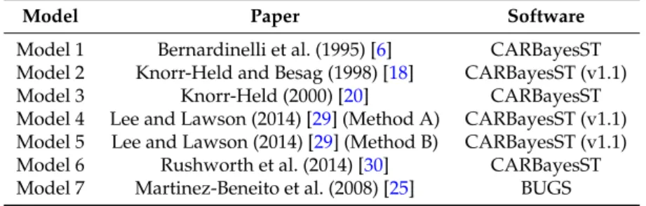
This section outlines an application of seven of the spatio-temporal models outlined above in order to illustrate the similarities and differences between each model. The seven models selected
are outlined in Table2. These models have been chosen because there is publicly available software
which allows us to apply them to our dataset. The nature of the software is outlined in Table2; six of
the models were applied using the CARBayesST R package [36], of which three are from version 1.1
of the package, and three are from the current version. The seventh model was fitted in OpenBUGS
which relates to hospitalisations due to ischaemic heart disease (IHD) in New South Wales, Australia between 2006 and 2013.
Table 2.Outline of the seven methods compared in this paper and the software used to fit them.
Model Paper Software
Model 1 Bernardinelli et al. (1995) [6] CARBayesST Model 2 Knorr-Held and Besag (1998) [18] CARBayesST (v1.1) Model 3 Knorr-Held (2000) [20] CARBayesST Model 4 Lee and Lawson (2014) [29] (Method A) CARBayesST (v1.1) Model 5 Lee and Lawson (2014) [29] (Method B) CARBayesST (v1.1) Model 6 Rushworth et al. (2014) [30] CARBayesST Model 7 Martinez-Beneito et al. (2008) [25] BUGS
3.1. Data
The study region is the state of New South Wales, which is located in south-eastern Australia. New South Wales is the most populous of the eight states and territories which make up Australia, with approximately 7.6 million residents. The state is divided into 199 administrative units known as statistical local areas (SLAs), which have been partitioned based on geographical and demographic factors. One of these administrative units, Lord Howe Island, is located around 600 km off the east coast of New South Wales, and will thus be excluded from this study. The SLA populations range from a minimum population of 752 to a maximum population of 145,865, with a median SLA population of 24,411.5. Almost two-thirds of New South Wales’ population lives in the Sydney metropolitan area, and this is reflected in the SLA structure: SLAs in the Sydney region have small areas and large populations, while more remote SLAs have very large areas but small populations.
The disease data are monthly counts of emergency hospitalisations due to ischaemic heart disease (IHD) in each SLA between January 2006 and June 2013. The data were provided by New South Wales Health, and correspond to the International Classification of Disease 10th revision codes I20–I25.
The dataset hasn = 198 areal units, with observations taken atJ = 90 time points. We also have
covariates relating to the patients’ age and gender, which are used to construct expected counts via internal standardisation. Population data and shapefiles were obtained from the Australian Bureau of Statistics (ABS).
In Figure1, we display the standardised incidence ratios (1) for the first and last January of
the study; note that January 2013 rather than June 2013 has been chosen in order to allow a direct
month-on-month comparison. Figure1a displays a map of the Standardised Incidence Ratios (SIRs) in
January 2006, and shows that there are substantial spatial variations in ischaemic heart disease risk,
with the risk appearing to be higher in the western and northern parts of New South Wales. Figure1b
shows a map of the SIRs in January 2013, and it is apparent that the disease risk has decreased overall during the study period. However, it appears that these decreases are not uniform across the region, and it appears that the risk is decreasing at a faster rate in the area around Sydney than in the more remote regions.
3.2. Model Comparison
Models 1–7 were applied to the data using the software outlined in Table2, with a month of the
year effect included as the only covariate in each model. Each model was fitted using Markov-Chain Monte Carlo (MCMC), with 10,000 iterations. In each case, the first 5000 iterations were discarded as burn-in, and the remaining 5000 were used to obtain our parameter estimates. The models were compared in terms of three key criteria: computing time, residual autocorrelation and model fit.
(a) (b)
Figure 1. Standardised incidence ratios (Yi/Ei) for statistical local areas in New South Wales. (a) Standardised incidence ratios for January 2006; (b) Standardised incidence ratios for January 2013.
The residual autocorrelation was measured using a spatio-temporal extension of the Moran’s I
statistic [38]. A spatio-temporal extension of this statistic was originally proposed as a descriptive
tool for spatio-temporal data [10], but here we propose a novel use of this statistic as a goodness-of-fit
test. Suppose our variable of interestY is measured for n areal units at J timepoints. Then, the
spatio-temporal Moran’s I statistic, MoranST, is given by
MoranST= nJ ∑n i=1 J ∑ j=1 n ∑ k=1 J ∑ l=1 ˜ w(ij,kl)(Yij−Y¯)(Ykl−Y¯) n ∑ i=1 J ∑ j=1 n ∑ k=1 J ∑ l=1 ˜ w(ij,kl) n ∑ i=1 J ∑ j=1 (Yij−Y¯)2 .
Here, ¯Yis the mean of the observed valuesYijand ˜w(ij),(kl)is a weight which accounts for the
spatio-temporal autocorrelation betweenyijandykl, defined as:
˜ w(ij),(kl)= wik, ifj=l, 1, ifi=kand|j−l|=1, 0, otherwise,
wherewikis a spatial weight which is equal to 1 if areasiandkare neighbours, and 0 otherwise.
This corresponds to a combination of the standard spatial neighbourhood matrix and a temporal autoregressive model with time lag 1. Any pair of observations which are either neighbours geographically and measured at the same timepoint, or measured at the same location one time point apart are considered to be “spatio-temporal neighbours” and are given a weight of 1. All other pairs of observations are given a weight of 0. A MoranST close to 1 corresponds to strong positive spatial autocorrelation, while a MoranST of 0 corresponds to complete spatial randomness.
We can adopt a similar technique to that used in spatial modelling, where the MoranST is used
to test for spatial correlation in the model residuals,e. The residuals of a model are defined as the
difference between the observed and fitted values, and can be computed aseij=Yij−Y˜ij, where ˜Yijis
the fitted value from the model for areaiat timej. A good spatio-temporal model should account for all
of the spatio-temporal trends in the data, and, in such cases, one would not expect any spatio-temporal correlation in the residuals. It is therefore possible to measure the quality of the model by computing the MoranST for the residuals; the best model is the one with the MoranST closest to zero.
The quality of the model fit is tested using the Deviance Information Criterion (DIC), which is
defined as DIC = ¯D+pd, where ¯Dis the mean posterior deviance andpdis the effective number of
parameters [39]. The posterior deviance would be minimised by the best fitting model (i.e., the most
effective number of parameters as a trade off. The model with the lowest DIC can be considered to provide the closest fit to the observed data.
4. Results
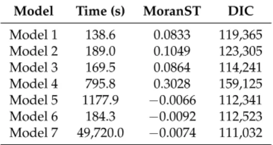
Table3displays the computational time, MoranST and DIC results for fitting each of the seven
selected models to our dataset. We can see that Models 1–3 and Model 6 can all fit the data in less than 200 s, while Models 4 and 5 take slightly longer, at 796 and 1178 s respectively. Model 7, the only model which was fitted using OpenBUGS rather than R, takes vastly longer to fit with our data: 14 h, compared to a maximum of 20 min for any of the other models. This increase in computing time may be prohibitive for some users, especially when working with datasets larger than this one. However, much of the time difference is likely down to the software implementation rather than the complexity of the model.
Table 3.Comparison of the performance of our seven models. Model Time (s) MoranST DIC
Model 1 138.6 0.0833 119,365 Model 2 189.0 0.1049 123,305 Model 3 169.5 0.0864 114,241 Model 4 795.8 0.3028 159,125 Model 5 1177.9 −0.0066 112,341 Model 6 184.3 −0.0092 112,523 Model 7 49,720.0 −0.0074 111,032
The MoranST scores for the residuals show that most of the models have done a reasonable job of accounting for the spatio-temporal trend in the dataset. The exception is Model 4, where a MoranST of 0.30 was obtained, which implies that there is still substantial spatio-temporal autocorrelation in the residuals after fitting the model. Model 5 has the MoranST score which is closest to zero—the value
of−0.0066 implies that there is almost no spatio-temporal autocorrelation present in the residuals,
which means the model has accounted for the trends in the data. Models 6 and 7 also perform well on
this measure, with MoranST scores of−0.0092 and−0.0074, respectively.
Models 5, 6 and 7 are also the ones which perform best in terms of the DIC. Model 7 has the lowest DIC with a value of 111,032, which implies that it provides the best fit to the observed data. Model 5 has the next best DIC (112,341), followed by Model 6, which has a DIC of 112,523. Based on these results, it appears clear that Models 5, 6 and 7 represent the three most promising approaches for our data. Model 7 has the best DIC score, but it requires a substantial undertaking in terms of computing time and therefore may not be an efficient choice in practice. With that in mind, Model 5 appears to be the best choice overall. It produces the best MoranST score and the next best DIC, and although it takes a little longer to fit than some of the other models, it was still able to handle our dataset within a reasonable timescale.
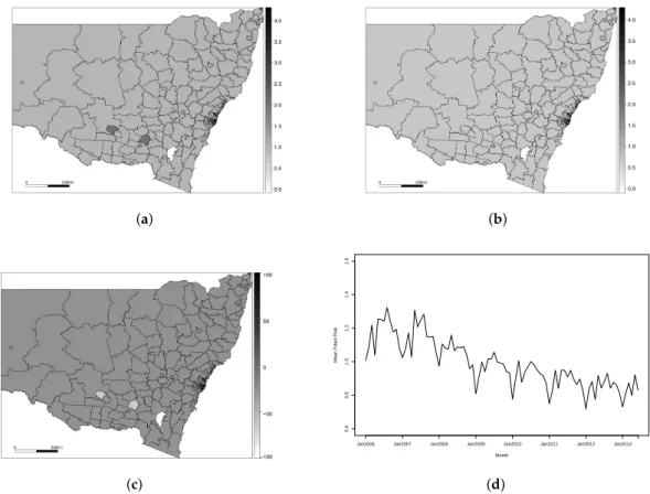
Figure2displays the results of fitting Model 5 to our dataset. Figure2a,b display the fitted
values for each areal unit in the first and last January of the study period (January 2006 and
January 2013, respectively), Figure2c displays the percentage change in disease risk from January 2006
to January 2013 and Figure2d displays the overall disease risk for the state of NSW in each month,
computed as the mean of the fitted risks in each subregion. We can see from Figure2a that the disease
levels are fairly constant across the region in January 2006, but Figure2b shows that, by January 2013,
there appears to be a more pronounced spatial pattern. This is reflected in the variances of the relative risks—in January 2006, the state-wide variance was 0.027, but, by January 2013, this increased to 0.077.
In January 2013, the relative risk of disease appears to be higher in the more remote regions further away from Sydney, although this pattern is not present in the border regions where edge
which shows small increases in fitted risk in these remote areas, while the areas closer to the city are
experiencing a decrease in risk. Figure2d shows that the risk fluctuates across the year, with higher
incidence of IHD in the winter months (June–August in Australia) and lower incidences in the summer (December–February). The average risk of IHD in New South Wales has decreased over the study period. The mean relative risk in January 2006 was 1.03, while the risk in January 2013 was 0.75. This corresponds to a mean decrease in risk of 28%, but it appears that these decreases have not been uniform across the state. The overall decrease in IHD risk in the state is a result of increased awareness and advancements in treatment and diagnosis, but these effects are less pronounced in remote areas where people do not have the same level of access to health care.
(a) (b) (c) 0.6 0.8 1.0 1.2 1.4 1.6 Month
Mean Fitted Risk
Jan2006 Jan2007 Jan2008 Jan2009 Jan2010 Jan2011 Jan2012 Jan2013
(d)
Figure 2.Results for Model 5. (a) Fitted IHD risks for January 2006; (b) Fitted IHD risks for January 2013; (c) Overall percentage change in fitted risks between January 2006 and January 2013; (d) Mean IHD risk in New South Wales by month.
For the purposes of comparison, and to show the benefit of a good model choice, we have included
a plot of the results for Model 4 in Figure3. Similar plots for each of the other five models are included
in the Supplementary Materials (Figures S1–S7, Tables S1 and S2). Model 4 was shown to be the poorest performing model and failed to capture the spatio-temporal trend in our dataset. It should be noted
that Models 4 and 5 come from the same paper [29], which proposes an underlying clustering model,
and outlines two different specifications for the spatio-temporal term. Model 4 proposes a piecewise constant spatio-temporal term for each cluster, while Model 5 allows for smoothing within a cluster.
It is apparent from Figure3that almost every element was classified in the same cluster for Model 4,
which led to a poor fit for the disease risk. The specification used in Model 5 allowed for much more spatial heterogeneity in the risk trends, which led to much better estimation of the risk pattern.
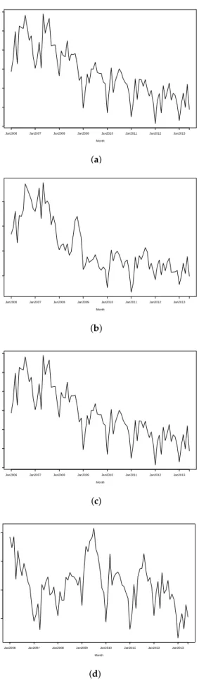
Figure4further illustrates the differences between these models by comparing the fitted trends
for two randomly selected subregions under each model. The selected areas were Lake Macquarie West, part of a coastal city around 150 km north of Sydney, and Uralla, an inland rural town about
450 km northwest of Sydney. Figure4a,c show that both regions have identical trends under Model 4
due to them being in the same cluster, while Figure4b,d show that Model 5 provides more flexibility
to fit individual trends for these regions.
(a) (b) (c) 0.6 0.8 1.0 1.2 1.4 1.6 Month
Mean Fitted Risk
Jan2006 Jan2007 Jan2008 Jan2009 Jan2010 Jan2011 Jan2012 Jan2013
(d)
Figure 3.Results for Model 4. (a) Fitted IHD risks for January 2006; (b) Fitted IHD risks for January 2013; (c) Overall percentage change in fitted risks between January 2006 and January 2013; (d) Mean IHD risk in New South Wales by month.
0.7 0.8 0.9 1.0 1.1 1.2 1.3 Month
Fitted IHD Risk
Jan2006 Jan2007 Jan2008 Jan2009 Jan2010 Jan2011 Jan2012 Jan2013
(a) 0.8 1.0 1.2 1.4 Month
Mean Fitted Risk
Jan2006 Jan2007 Jan2008 Jan2009 Jan2010 Jan2011 Jan2012 Jan2013
(b) 0.7 0.8 0.9 1.0 1.1 1.2 1.3 Month
Fitted IHD Risk
Jan2006 Jan2007 Jan2008 Jan2009 Jan2010 Jan2011 Jan2012 Jan2013
(c) 0.6 0.7 0.8 0.9 Month
Mean Fitted Risk
Jan2006 Jan2007 Jan2008 Jan2009 Jan2010 Jan2011 Jan2012 Jan2013
(d)
Figure 4.Fitted IHD trends for two randomly selected subregions using Models 4 and 5. (a) Trend for Lake Macquarie West using Model 4; (b) Trend for Lake Macquarie West using Model 5; (c) Trend for Uralla using Model 4; (d) Trend for Uralla using Model 5.
5. Discussion
Spatio-temporal models are used for a wide range of applications and data types,
and, consequently, the literature is quite diffuse. Section2.2provides an overview of these models
and outlines similarities and differences between existing models. We have shown that these spatio-temporal models can be broken down into spatial, temporal and spatio-temporal terms, and we have identified the different structures used for these terms within different modelling frameworks. The early spatio-temporal literature tended to favour simpler models, often omitting a spatio-temporal interaction term, but we have identified that such a term can be useful in cases where the temporal trends in disease risk vary from region to region. Recent developments in computing power have allowed more and more complex spatio-temporal models to be fitted, and many contemporary approaches can account for such spatio-temporal differences.
In Section3, we compared seven spatio-temporal models by applying them to data for ischaemic
heart disease (IHD) hospital admissions in New South Wales, Australia. This application showed
that the model proposed by Lee and Lawson [29] performed best in terms of accounting for the
spatio-temporal trends present in the data, as measured by the MoranST score. The model proposed
by Martinez-Beneito et al. [25] provides a slightly better fit in terms of DIC, but a major limitation
of this method is the computing time required for the existing software for the approach. Based on
these results, we selected the Lee and Lawson [29] approach using within-cluster smoothing as the
best model for our dataset.
6. Conclusions
The spatio-temporal term in the Lee and Lawson [29] model allowed us to accurately capture the
variation in the temporal trends across the region. The clustering structure present in this algorithm means that extreme risks are not necessarily smoothed towards the global mean, an advantage in cases where one would like to identify high (or low) risk areas. We identified that IHD risk in New South Wales decreased by around 28% between 2006 and 2013, and that disease risk was higher in the winter months than the summer months. We also identified that the decrease in IHD risk is not uniform across the state; for many remote areas in the north and west of the state, the risk stayed constant or even increased slightly. People in these remote areas have less access to healthcare than those in urban areas, and therefore have not experienced the same benefits of increased awareness and improved treatment and diagnosis of IHD.
The field of spatial modelling has grown substantially over the last couple of decades, aided by recent developments in computational power and the collection and publication of larger and more complex datasets. In particular, applications in epidemiology, ecology and meteorology have become increasingly common because of the importance of there being model changes in spatial patterns over time to identify trends. The increasing shift towards ‘big data’ has clear implications in spatio-temporal modelling, and it seems likely that the development of parallelisable spatio-temporal models will be the next key area of development.
Supplementary Materials: The following are available online at www.mdpi.com/1660-4601/14/2/146/s1. Figure S1: Results for Model 1, Figure S2: Results for Model 2, Figure S3: Results for Model 3, Figure S4: Results for Model 4, Figure S5: Results for Model 5, Figure S6: Results for Model 6, Figure S7: Results for Model 7, Table S1: Outline of the seven methods compared in this paper and the software used to fit them, Table S2: Comparison of the performance of our seven models.
Acknowledgments: Both authors were funded by the Australian Research Council Centre of Excellence for Mathematical and Statistical Frontiers (ACEMS). The authors gratefully acknowledge helpful suggestions made by the two referees, which have greatly improved the content of this paper.
Author Contributions:Craig Anderson carried out the literature review and developed the MoranST approach for goodness of fit; Louise M. Ryan obtained the data; Craig Anderson developed the software and performed the analysis. Both authors contributed to the analysis of the results and the subsequent discussion section. Craig Anderson wrote the paper with input from Louise M. Ryan.
References
1. Best, N.; Richardson, S.; Thomson, A. A comparison of Bayesian spatial models for disease mapping.
Stat. Methods Med. Res.2005,14, 35–59.
2. Lee, D.; Shaddick, G. Spatial modeling of air pollution in studies of its short-term health effects.Biometrics
2010,66, 1238–1246.
3. Ver Hoef, J.; Peterson, E.; Theobald, D. Spatial statistical models that use flow and stream distance.
Environ. Ecol. Stat.2006,13, 449–464.
4. Rodriguez-Iturbe, I.; Mejia, J. The Design of Rainfall Networks in Time and Space. Water Resour. Res.
1974,10, 713–728.
5. Cressie, N.; Wikle, C.Statistics for Spatio-Temporal Data; Wiley: Hoboken, NJ, USA, 2011.
6. Bernardinelli, L.; Clayton, D.; Pascutto, C.; Montomoli, C.; Ghislandi, M.; Songini, M. Bayesian analysis of space–time variation in disease risk. Stat. Med.1995,14, 2433–2443.
7. MacNab, Y.; Dean, C.B. Autoregressive Spatial Smoothing and Temporal Spline Smoothing for Mapping Rates.Biometrics2001,57, 949–956.
8. Huang, H.; Cressie, N.; Gabrosek, J. Fast, Resolution-Consistent Spatial Prediction of Global Processes from Satellite Data. J. Comput. Graph. Stat.2002,11, 63–88.
9. Kammann, E.; Wand, M. Geoadditive models. J. R. Stat. Soc. Ser. C Appl. Stat.2003,52, 1–18.
10. Chen, S.-K.; Wei, W.; Mao, B.-H.; Guan, W. Analysis on urban traffic status based on improved spatio-temporal Moran’s I.Acta Phys. Sin.2013,62, 148901. (In Chinese, abstract In English)
11. Besag, J.; York, J.; Mollié, A. Bayesian image restoration, with two applications in spatial statistics. Ann. Inst. Stat. Math.1991,43, 1–20.
12. Earnest, A.; Morgan, G.; Mengersen, K.; Ryan, L.; Summerhayes, R.; Beard, J. Evaluating the effect of neighbourhood weight matrices on smoothing properties of Conditional Autoregressive (CAR) models.
Int. J. Health Geogr.2007,6, 1–12.
13. Cressie, N.Statistics for Spatial Data, revised edition ed.; Wiley: Hoboken, NJ, USA, 1993.
14. Leroux, B.; Lei, X.; Breslow, N. Statistical Models in Epidemiology, the Environment and Clinical Trials. InEstimation of Disease Rates in Small Areas: A New Mixed Model for Spatial Dependence; Halloran, M., Berry, D., Eds.; Springer: New York, NY, USA, 1999; pp. 135–178.
15. Waller, L.; Carlin, B.; Xia, H.; Gelfand, A. Hierarchical Spatiotemporal Mapping of Disease Rates. J. Am. Stat. Assoc.1997,92, 607–617.
16. Xia, H.; Carlin, B. Spatio-Temporal Models with Errors in Covariates: Mapping Ohio Lung Cancer Mortality.
Stat. Med.1997,17, 2025–2043.
17. Chib, S. Bayes regression with autoregressive errors: A Gibbs sampling approach. J. Econom.
1993,58, 275–294.
18. Knorr-Held, L.; Besag, J. Modelling risk from a disease in space and time.Stat. Med.1998,17, 2045–2060. 19. Bohning, D.; Dietz, E.; Schlattmann, P. Space–time mixture modelling of public health data. Stat. Med.
2000,19, 2333–2344.
20. Knorr-Held, L. Bayesian modelling of inseparable space–time variation in disease risk. Stat. Med.
2000,19, 2555–2567.
21. Bohning, D. Empirical Bayes estimators and non-parametric mixture models for space and timespace disease mapping and surveillance.Environmetrics2003,14, 431–451.
22. Congdon, P.; Southall, H. Trends in inequality in infant mortality in the north of England, 1921 to 1973, and their association with urban and social structure.J. R. Stat. Soc. Ser. A2005,168, 679–700.
23. MacNab, Y. Spline smoothing in Bayesian disease mapping. Environmetrics2007,18, 727–744.
24. Kottas, A.; Duan, J.; Gelfand, A. Modeling disease incidence data with spatial and spatio-temporal Dirichlet process mixtures. Biometr. J.2008,1, 29–42.
25. Martinez-Beneito, M.; Lopez-Quilez, A.; Botella-Rocamora, P. An autoregressive approach to spatio-temporal disease mapping. Stat. Med.2008,27, 2874–2889.
26. Ugarte, M.D.; Goicoa, T.; Militino, A.F. Spatio-temporal modelling of mortality risks using penalized splines.
Environmetrics2010,21, 270–289.
27. Torabi, M.; Rosychuk, R. Spatio-temporal modelling using B-spline for disease mapping: Analysis of childhood cancer trends.J. Appl. Stat.2011,38, 1769–1781.
28. Lawson, A.; Choi, J.; Cai, B.; Hossain, M.; Kirby, R.; Liu, J. Bayesian 2-stage space time mixture modeling with spatial misalignment of the exposure in small area health data. J. Agric. Biol. Environ. Stat.2012,17, 417–441. 29. Lee, D.; Lawson, A. Cluster detection and risk estimation for spatio-temporal health data. arXiv
2014, arXiv:1408.1191.
30. Rushworth, A.; Lee, D.; Mitchell, R. A spatio-temporal model for estimating the long-term effects of air pollution on respiratory hospital admissions in Greater London. Spat. Spatio-Temporal Epidemiol.
2014,10, 29–38.
31. De Boor, C. On Calculation With B-splines. J. Approx. Theory1972,6, 50–62.
32. MacNab, Y.; Gustafson, P. Regression B-spline smoothing in Bayesian disease mapping: With an application to patient safety surveillance. Stat. Med.2007,26, 4455–4474.
33. Green, P.; Silverman, B.Nonparametric Regression and Generalized Linear Models; Chapman and Hall: London, UK, 1994.
34. Eilers, P.; Marx, B. Flexible smoothing with B-splines and penalties.Stat. Sci.1996,11, 89–121.
35. Lee, D.; Durban, M. P-spline ANOVA-type interaction models for spatio-temporal smoothing. Stat. Model.
2011,11, 49–69.
36. Lee, D.; Rushworth, A. CARBayesST: Poisson Log-Linear Models with Spatio-Temporal Random Effects. R Package. 2014. Available online: https://github.com/barryrowlingson/CARBayesST (accessed on 1 February 2017).
37. Martinez-Beneito, M. BUGS Code for AR1 Model. Available online: http://www.uv.es/ mamtnez/AR1.txt (accessed on 1 February 2017).
38. Moran, P. Notes on Continuous Stochastic Phenomena. Biometrika1950,37, 17–23.
39. Spiegelhalter, D.; Best, N.; Carlin, B.; Van der Linde, A. Bayesian measures of model complexity and fit. J. R. Stat. Soc. Ser. B2002,64, 583–639.
c
2017 by the authors; licensee MDPI, Basel, Switzerland. This article is an open access article distributed under the terms and conditions of the Creative Commons Attribution (CC BY) license (http://creativecommons.org/licenses/by/4.0/).