Edited by: Emre O. Neftci, University of California, Irvine, United States Reviewed by: Siddharth Joshi, University of Notre Dame, United States Fabio Stefanini, Columbia University, United States *Correspondence: Bernabé Linares-Barranco [email protected]
†These authors have contributed
equally to this work
Specialty section: This article was submitted to Neuromorphic Engineering, a section of the journal Frontiers in Neuroscience Received:05 December 2017 Accepted:04 September 2018 Published:15 October 2018 Citation: Yousefzadeh A, Stromatias E, Soto M, Serrano-Gotarredona T and Linares-Barranco B (2018) On Practical Issues for Stochastic STDP Hardware With 1-bit Synaptic Weights. Front. Neurosci. 12:665. doi: 10.3389/fnins.2018.00665
On Practical Issues for Stochastic
STDP Hardware With 1-bit Synaptic
Weights
Amirreza Yousefzadeh†, Evangelos Stromatias†, Miguel Soto, Teresa Serrano-Gotarredona and Bernabé Linares-Barranco*
Instituto de Microelectrónica de Sevilla (IMSE-CNM), CSIC and Universidad de Sevilla, Sevilla, Spain
In computational neuroscience, synaptic plasticity learning rules are typically studied using the full 64-bit floating point precision computers provide. However, for dedicated hardware implementations, the precision used not only penalizes directly the required memory resources, but also the computing, communication, and energy resources. When it comes to hardware engineering, a key question is always to find the minimum number of necessary bits to keep the neurocomputational system working satisfactorily. Here we present some techniques and results obtained when limiting synaptic weights to 1-bit precision, applied to a Spike-Timing-Dependent-Plasticity (STDP) learning rule in Spiking Neural Networks (SNN). We first illustrate the 1-bit synapses STDP operation by replicating a classical biological experiment on visual orientation tuning, using a simple four neuron setup. After this, we apply 1-bit STDP learning to the hidden feature extraction layer of a 2-layer system, where for the second (and output) layer we use already reported SNN classifiers. The systems are tested on two spiking datasets: a Dynamic Vision Sensor (DVS) recorded poker card symbols dataset and a Poisson-distributed spike representation MNIST dataset version. Tests are performed using the in-house MegaSim event-driven behavioral simulator and by implementing the systems on FPGA (Field Programmable Gate Array) hardware.
Keywords: spiking neural networks, spike timing dependent plasticity, stochastic learning, feature extraction, neuromorphic systems
1. INTRODUCTION
One goal of neuromorphic engineering is to map efficiently neurocomputational algorithms onto compact, low power, and fast hardware, while preserving satisfactorily the functionalities of the theoretical algorithms. The main first question (digital) hardware neuromorphic engineers ask themselves is about the minimum required bits to represent parameters and states. Theoretical neurocomputists, which use as tools conventional computers, use typically the full 64-bit floating point precision available to develop and study their algorithms. However, using 64-bit floating point precision for neuromorphic hardware, where typically massive parallelism is physically implemented, imposes a severe resources penalty not only for memory usage, but also for all computing and communication resources. Because of this, for example, the SpiNNaker spiking neuromorphic platform, although it uses 32-bit precision hardware, it restricts itself to integer arithmetic (instead of floating point), thus introducing some hardware simplifications (Furber et al., 2014). In another example, the TrueNorth platform (Cassidy et al., 2013) is built upon multiple
256×256 1-bit synaptic weight crossbars, although it includes extra circuitry to allow assigning up to four possible 8-bit values to the synapses (with some restrictions). In the world of non-spiking Deep Neural Networks (DNN), where there is now a strong quest for providing dedicated efficient hardware (Chen et al., 2016; Sim et al., 2016; Bong et al., 2017; Whatmough et al., 2017; Biswas and Chandrakasan, 2018; Gonugondla et al., 2018; Khwa et al., 2018), some theorists are studying ways to reduce bit precision of the weights down to 1-bit (Courbariaux et al., 2015; Rastegari et al., 2016) to help simplifying hardware. Here we focus on spiking neural network (SNN) hardware capable of on-line unsupervised learning through Spike-Time-Dependent-Plasticity (STDP). In a previous work (Yousefzadeh et al., 2017) we implemented deterministic STDP hardware with 9-bit resolution for the weights. Our goal here is to obtain a working learning (stochastic) STDP layer by restricting the weights to 1-bit precision (“0” or “1”) for both learning and inference phases. For this, we consider a feed-forward neural system made of two layers. The first layer, restricted to 1-bit weights, uses stochastic STDP unsupervised learning for learning representative features. The second layer uses some trainable SNN classifier with supervised learning for pattern classification (Stromatias et al., 2017; Yousefzadeh et al., 2017). Interestingly, the conventional full-precision additive STDP learning rule will result in a bimodal weight distribution after learning (Barbour et al., 2007; Galluppi et al., 2015). This means that, even in the case of graded synaptic weights, the final weight values tend to saturate to the minimum (disconnected) or maximum (fully connected) value.
STDP was originally proposed by Gerstner et al. (1993), evolving later on to successfully learn hidden spiking patterns (Masquelier et al., 2008), to perform competitive spike pattern learning (Masquelier et al., 2009), to achieve reward modulated (pseudo-supervised) learning (Mozafari et al., 2017), or to be successfully applied to deep spiking neural networks (Kheradpisheh et al., 2018). Surprisingly, experimental evidence of STDP in biological synapses was reported by neuroscientists shortly after proposing the computational algorithms for the first time (Markram et al., 1997; Bi and Poo, 1998, 2001; Zhang et al., 1998; Feldman, 2000; Mu and Poo, 2006; Cassenaer and Laurent, 2006; Jacob et al., 2007). However, STDP works typically by performing very small weight changes, which implies high resolution for the weights, consequently imposing high hardware resources demands for memory, computing, and communication circuits. Most of the neuromorphic hardware designs use on-chip memory to reduce power consumption (Cassidy et al., 2013; Davies et al., 2018)1 and therefore memory is a limiting factor for the number of neurons and synaptic connections. By using 1-bit synaptic weights, not only the memory, but all the processing elements inside the chip will be much simpler. Reducing weight resolution from 9-bit to 1-bit, should in principle allow for about one order of magnitude reduction
1The dominant power is typically burnt in the continuous and massive data transfers between computing circuits and memory circuits. If computing and memory circuits are in separate chips, data transfer power is multiplied by one or two orders of magnitude.
in memory, computing, communication resources and power consumption. When restricting to 1-bit weights, one option is to consider some type of stochastic weight update. This is, instead of applying a given weight change from the STDP rule, one changes the weight from either “0” to “1” or from “1” to “0” with a probability given by the STDP rule. This idea has already been used before. Suri et al. (2013) applied it to cluster vehicle trajectories recorded with spiking retinas (Dynamic Vision Sensors -DVS-) (Lichtsteiner et al., 2008; Posch et al., 2011; Serrano-Gotarredona and Linares-Barranco, 2013; Son et al., 2017; Guo et al., 2017) into highway lane segments.Seo and Seok (2015)applied it to simple classification problems, but found out that they could not learn to separate more than five patterns. Here we want to learn to classify either DVS recorded poker card symbols (Soto, 2017) or a spiking representation of the MNIST dataset (LeCun et al., 1998). At the beginning, we were not able to obtain any reasonable learning by simply applying an STDP binary update with stochasticity. It was not until we started applying some additional “tricks” that we started to observe the formation of characteristic features together with overall reasonable accuracy results. These “tricks” were weight normalization, individual neuron threshold adjustment, or using separate thresholds for learning and inference.
Since there is no other work in the literature reporting classification accuracy results for 1-bit weights STDP feature extraction (FE) layers, we compare with purely random 1-bit weights FE layers. It is well-known that it is possible to build excellent performance pattern learning and classification systems by using a sufficiently large hidden FE layer with random weights, followed by a trainable high performance classification layer (Huang et al., 2006). Based on this, we compare our STDP systems with a “parallel” one using the same classifier output layer and a hidden layer with the same number of neurons but with 1-bit random weights. As shown later in the section 3, there is always a consistent improvement when using STDP with respect to using pure random weights, although this improvement reduces as the number of hidden layer neurons increases.
Throughout the paper we will use always a very simple neuron model, namely, the leak (or piece-wise linear-leak) integrate-and-fire (LIF) model, together with instantaneous synapses (Camuñas-Mesa et al., 2010, 2011, 2012; Pérez-Carrasco et al., 2013; Serrano-Gotarredona et al., 2015), restricted to positive neural state values.
The paper is structured as follows. In the section 2 we will first include a quick review on different STDP rules, signaling the difference between more conventional time-based STDP rules vs. less conventional order-based STDP rules, which we will use here. Then we will briefly explain how we “engineer” STDP and, in particular, stochastic STDP with 1-bit weights by adding some “tricks.” Then we present quickly two previously reported spiking classifiers we have used, followed by a quick description of the software and hardware experimentation platforms used. In the section 3 we provide software and hardware results for three experiments. A first experiment is a very simple 4-neuron system that replicates a biological experiment of visual orientation tuning (Bienenstock et al., 1982; Moore and Freeman, 2012; Jeyabalaratnam et al., 2013). It is a very
simple starting point used as reference in other computational studies (Galluppi et al., 2015). The second experiment learns to classify poker card symbols (Soto, 2017) recorded with a spiking retina Dynamic Vision Sensor (DVS) (Serrano-Gotarredona and Linares-Barranco, 2013). The third experiment learns to classify the MNIST dataset. More specifically, a spiking version of it, obtained by generating Poisson distributed spike trains from the original pixel gray levels. This is a common technique for converting static images to synthetic spike-trains and has been used in a number of previous studies (O’Connor et al., 2013; Querlioz et al., 2013; Diehl et al., 2015; Diehl and Cook, 2015; Galluppi et al., 2015; Stromatias et al., 2017). Finally, the paper finishes by presenting some Discussions and Conclusions.
2. MATERIALS AND METHODS
2.1. Review of Some STDP Rules
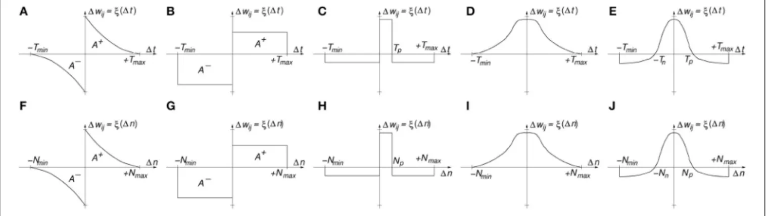
Figure 1Ashows a typical STDP update functionξ(1t), where
1tis the time difference between a post-synaptic spike at time
tpost and a pre-synaptic spike at timetpre. In biology, the time
window [−Tmin,Tmax] is typically in the range of about 100 ms,
although in artificial systems one can adjust this time window to the dynamics of the data spikes. Figures 1B–E illustrate other STDP learning functions ξ() that have been used in the computational neuroscience literature and/or observed in biology. For example,Figure 1Bis a simplification ofFigure 1A
that provides a relatively similar outcome as long as the ratio of the areas under the positive A+ and negative A− branches is preserved. Figure 1C shows an STDP learning function ξ() where potentiation is applied only for a narrow positive time window 0 < 1t < Tp, otherwise there will be depression. An
interesting, powerful and widely used extension of this learning function is when+Tmax → +∞and−Tmin → −∞(Bichler et al., 2012; Suri et al., 2013; Querlioz et al., 2013). This is, whenever there is a post-synaptic spike, all synapses connecting to this destination neuron will be depressed by a fixed amount, except those who have transmitted a pre-synaptic spike during a prior time windowTpwhich will undergo a potentiation2. Let
us call this type of STDP “undiscriminating depressing STDP.” This implementation requires less resources, as discussed later.
Figure 1Dis another interesting STDP version, where synapses are potentiated whenever pre- and post-synaptic spikes are more or less coincident in time, irrespective of which happens first. This “symmetric hebbian” STDP learning has also been found in some biological synapses (Roberts and Bell, 2002).Figure 1E
is a type of symmetric “undiscriminating depressing” version of
Figure 1D, also found in biology (Dan and Poo, 1998).
The STDP functionsξ(1t) inFigures 1A–Fare all time-based (function of1t). In practical implementations (like digital HW or SW algorithms), one keeps a list of the pre- and post-synaptic spikes with their respective timestamps for later computation
2Strictly speaking, the correct formulation should say−T
min=0. This is because
for1t <0 (pre after post), a new arriving pre-synaptic spike checks the list of prior post-synaptic spikes to perform weight update. This means, that for every pre-synaptic spike, all synapses connecting to this pre-synaptic neuron should also be depressed. However, this action is not taken (Bichler et al., 2012; Querlioz et al., 2013; Roclin et al., 2013; Suri et al., 2013).
of the STDP function for each synaptic connection and corresponding update. Some neurocomputational researchers have proposed and successfully implemented time-abstracted versions of the STDP functionξ(), where the time variable has been removed and substituted by the order of the occurrence of the spikes (Thorpe and Gautrais, 1998; Masquelier and Thorpe, 2007; Bichler et al., 2012; Roclin et al., 2013). This way, each spike is not associated to a timestamp, but to an integer number
nindicating its rank or order of occurrence. In this abstracted representation the time difference between consecutive spikes is irrelevant, and it only matters which spikes appear after or before each other. This is called “order-based” STDP and the learning function is nowξ(1n). In order-based STDP implementations one simply needs to keep track of an ordered list of pre- and post-synaptic spikes, without any timestamp. One can keep one single ordered list of the full system, separate ordered lists for sub-populations of the system, or even separate ordered lists for each synapse. When keeping track of the ordered lists, one should set a maximum number N of events to keep in the list, so that STDP learning is only driven by reasonably recent events. Figures 1F–J show the equivalent order-based STDP learning function versions of those shown inFigures 1A–E. One interesting feature of order-based STDP is that learning self-adapts to the dynamics of the neural activity. This is radically different to what happens in biology, where STDP is always time-based and consequently tuned to a specific range of time constants and dynamics. In order-based STDP the learning will occur in the same way, independently of the speed and dynamics with which events occur. If all spike timestamps are multiplied by the same constant, their ordering will be the same and consequently learning remains unchanged. Therefore, order-based STDP self-adapts to the speed and dynamics of the events.
2.2. Engineering STDP
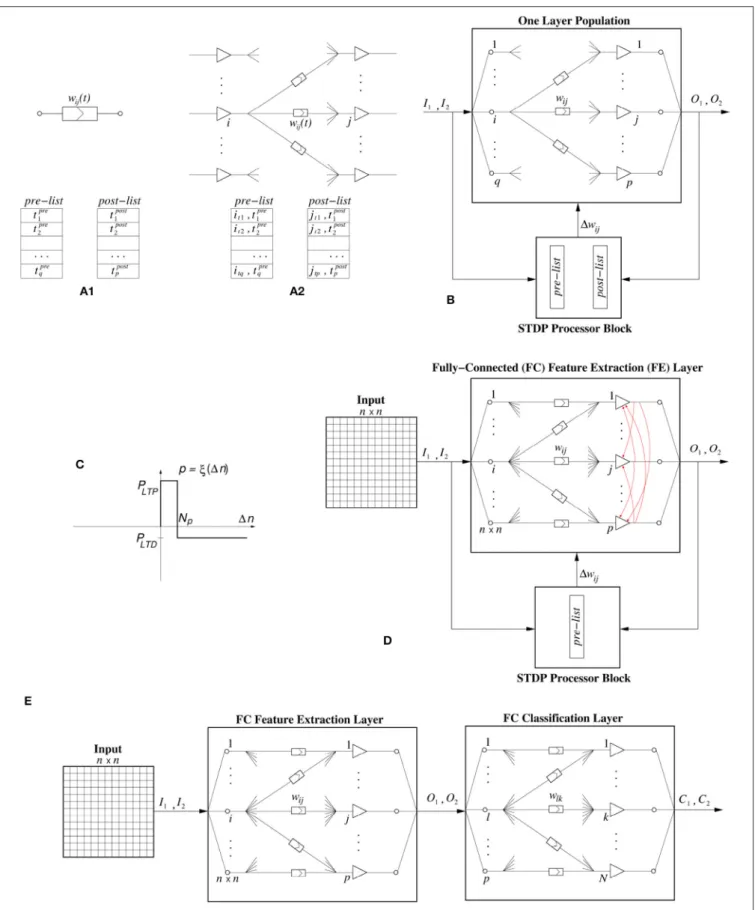
In software as well as in hardware, STDP can be computed in many different ways. Here we follow an event-driven approach for both the software as well as the digital hardware implementation. This way, computations are not performed time-step by time-step, but only when an event is generated and transmitted. One way of computing STDP in an event-driven simulation is by keeping a bounded list of pre- and post-synaptic events. This is, for example, illustrated in Figure 2A1 for an individual synapse. Every time a pre-synaptic event is received by a synapse, its time of occurrence is stored in a pre-list or pre-buffer. Ift is the present time, events are kept in the pre-synaptic list as long ast−tpren ≤ Tmax. Similarly, whenever the
post-synaptic neuron generates a spike, its time of occurrence is stored in a post-list or post-buffer, where events are kept as long ast −tpostm ≤ Tmin. For every new pre-synaptic event at time
t, it is stored in the pre-list, the post-list is scanned, and1wij
is computed by using the correspondingξ(tmpost −t) function.
Similarly, for every new post-synaptic event at timet, it is stored in the post-list, the pre-list is scanned and1wijis computed using
ξ(t−tpren ). Depending on the type of STDP rule, one can choose
to update a synapse for all the events in the list, or only for the most recent one(s).
FIGURE 1 | (A)Classic time-based STDP(B)Rectangular time-based STDP,(C)Narrow Potentiation time-based STDP,(D)Symmetric Hebbian Potentiating only time-based STDP,(E)Symmetric Hebbian with Narrow Potentiation time-based STDP,(F)Classic order-based STDP(G)Rectangular order-based STDP,(H)Narrow Potentiation order-based STDP,(I)Symmetric Hebbian Potentiating only order-based STDP,(J)Symmetric Hebbian with Narrow Potentiation order-based STDP.
However, keeping a separate pre- and post-list for each individual synapse is costly for both software and hardware implementations. Consequently, normally one keeps one pre-and one post-list for a full population, as illustrated in
Figure 2A2, including the indexes i and j of pre- and post-synaptic neurons.
For the cases of order-based STDP rules, the pre- and post-list will not contain any time information, but just the indexes of the pre- and post-synaptic neurons in the proper order. The number of events kept in each list is a fixed integer number (which we will call “buffer size”).
Note that if one setsTmin=0 orNmin=0, only the pre-list is
required. Similarly, ifTmax=0 orNmax=0, only the post-list is
required.
In the implementations (for both software and hardware) reported in this paper, we will keep a separate “STDP processor” connected to a neuron population containing its input synapses, as illustrated inFigure 2B. In this approach, the STDP processor receives a replica of, both, all pre-synaptic eventsIkand all
post-synaptic eventsOl. For each new event it checks the opposite list
of stored events, and sends a kind of1wijcommand/event to the
neuron population to update each of thewijweights that requires
STDP update.
2.3. Engineering Stochastic STDP With
1-bit Weights
When restricting to 1-bit weights, it is no longer possible to consider small values for1wij. Weights change directly from “0”
to “1,” or vice versa. In this case, one can consider a stochastic version of STDP by simply substituting the learning functions in
Figure 1to provide a given signed probability3for potentiation
or depression. The weights are directly set to “1” (ON state) or “0” (OFF state) depending on the resulting probability and sign of function ξ(). For example, if ξ(1t) or ξ(1n) is equal to a
3Strictly speaking, probabilities are positive numbers. Here we consider that a positive probability provides a probability for potentiation, and a negative probability provides a probability for depression.
positive probabilityp(with 0 ≤ p ≤ 1), then after generating a random numberx(with 0 ≤ x ≤ 1), if x ≤ pthe weight will be set to “1,” otherwise it will remain unchanged. In the case of negative probability p = ξ() values (with 0 ≥ p ≥ −1), after generating the random numberx (with 0 ≤ x ≤ 1), if
x ≤ |p| the weight will be set to “0,” otherwise it will remain unchanged.
The proposed STDP implementation with stochastic updates is of the type “undiscriminating depressing” order-based STDP. Therefore, only the pre-list is kept and whenever a neuron generates a post-synaptic event, the synapses connecting to this neuron in the pre-list are potentiated while all remaining synapses connecting to this neuron are depressed. The STDP learning function is shown inFigure 2C, and is a particular case ofFigure 1CforNmin =0 andNmax= ∞, but with the vertical
axis indicating either long term potentiation probabilityPLTP
or long term depression probabilityPLTD. ParameterNp is the
“buffer size” of the pre-list of the population, while1nis the event index in the pre-list of the population.
Additionally, we incorporate a number of additional “tricks” which help to obtain representative features4, while allowing the use of larger probabilities. This way, the learning is fast but stable. These “tricks” are the following:
1. Individually incrementing neuron thresholds xthj.During
learning, every time a neuron j produces an output event, its thresholdxthjis incremented. This is because its receptive
field weights will become more selective to a given feature, or equivalently, it has specialized to recognize a given feature, and consequently should give more chances to other neurons to pick up other features. To do so, its threshold is increased so that other still unspecialized (or less specialized) neurons have better chances to fire. This implements a form ofhomeostasis
(Querlioz et al., 2013; Diehl and Cook, 2015). Typically, we increment a threshold by “1,” but it could be incremented by any predetermined integer number.
4Obtaining representative features should make the task of the classifier layer more easy.
FIGURE 2 | (A)STDP computation.(A1)By keeping a pre- and a post-synaptic event list per synapse,(A2)by keeping a pre- and a post-synaptic event list per neuron population with its input synapses.(B)STDP computation block assigned to a neuron population with its input synapses.(C)Stochastic STDP learning function.(D)The neural network topology used in this work for the fully-connected FE (feature extraction) hidden layer, wherepis its size. The red arrows represent the lateral inhibition that is implemented internally.(E)Event-Driven System Topology used in this paper when the experiments require a FE layer and a Classifier layer.
2. Weight Normalization. The sum of the weights Wsum = P
iwijconnecting to a neuronj, is maintained constant5. This
can be enforced deterministically after each random update, or stochastically by readjusting the probability depending on the instantaneous value ofWsum. If deterministic, the sum of
weights will be kept constant at any time, but if stochastic, the sum will randomly wander around the target value. Without this “trick” some neurons become dead (null synapses) or over-activated (having too many active synapses), resulting in unstable learning. Different neuron populations can have differentWsum.
3. Neuron thresholdxthjsaturation.The thresholdxthj of each
neuron in a plastic population is not allowed to exceed a predefined maximum threshold xthmax. This feature was
introduced because we noticed that populations with fewer number of neurons for a given task produced very large final thresholds and ended up generating no events for an input sample during the testing phase.
4. Separate neuron thresholds for STDP process and for inference process.The idea is to keep for each neuron two different neuron states with their corresponding thresholds, one used for STDP weights updates and the other used for inference. Each incoming event updates both states. For inference the thresholds can be kept constant for simplicity, or they can also be adaptive as mentioned above. For STDP, the threshold is increased every time it is reached. Reaching the STDP threshold triggers weight update. By decoupling STDP and inference, neural activity can be kept high (which may improve learning at the next layer), while slowing down STDP learning as the neuron becomes more selective. Note that for STDP and inference processes to be decoupled, they should not have all characteristics equal (threshold increment, initial conditions). This “trick” is only implemented in the hardware implementations. The reason is that in the hardware versions, training is fully on-line. This is, all layers are trained simultaneously. Consequently, by separating inference and STDP thresholds, firing activity is kept high all the time, helping to accelerate learning in later layers. For the software versions, since learning is performed off-line, layers are trained sequentially.
5. Lateral Inhibition. When a population receives an input event, several neurons can reach their threshold and fire. However, we only allow one to fire. The rest of neurons in the population will be reset. This way we are implementing a form of internal lateral inhibition which resembles a winner-takes-all (WTA) (Maass, 2000) layer. This lateral antagonism forces competition between the neurons. It can be also more efficient for hardware designs, compared to the alternative method of using recurrent inhibitory soft connections.
5In conventional neural networks (with weights of higher resolution) scaling the weights by a factorαis equivalent to scaling the threshold by 1/α(previous “trick”). But here weights are either “0” or “1” and cannot be scaled. It is the total number of weights with value “1” that is kept constant. AlsoWsumis the same for
all neurons in the population, while in the previous “trick” each neuron can change its threshold separately.
6. List Flushing. After one output event is produced by a given neuron, the present list of stored pre-synaptic events of the population can be fully emptied. This way, the most recent history that triggered this output event is the only one used to contribute to learning for this output event. It will not contribute to learning induced by other output events. Although this “trick” had no impact on the learning of the systems tested (accuracy results are practically identical whether “list flushing” was active or not6), for the hardware implementations it introduced relevant simplifications, as explained later in the hardware description of the STDP unit. In the software experiments, training was done off-line, layer by layer, thus decoupling the learning processes between layers. Therefore, as soon as the STDP learning process was finished in the FE layer, the weights were fixed to their final values and each neuron threshold (xthj) was set to its last final
threshold. Also, the lateral inhibition between neurons of the same population was disabled. After this, the classifier layer was trained independently. However, if an application requires a hardware implementation with learning, it is because on-line learning is required. Otherwise, one would implement a pure inferring hardware which is simpler and consequently more efficient (Chen et al., 2016; Sim et al., 2016; Bong et al., 2017; Whatmough et al., 2017; Biswas and Chandrakasan, 2018; Khwa et al., 2018). Therefore, for our hardware tests we always implemented simultaneous on-line learning for all layers.
2.4. Network Architecture
The neural network topology used throughout this work can be seen inFigure 2D. It is a fully connected topology, where the first layer is the input layer, whose sizen×ndepends on the size of the particular data set. The second layer, which is a fully connected (FC) Feature Extraction (FE) layer, consists of a population of spiking neurons. Attached to the plastic FE neural layer is the stochastic binary weighted STDP processor block which receives two inputs, one from the presynaptic input layer and one from the post-synaptic FE layer. The STDP block sends weight update events 1wij with the indexes of the synapses that need to be
potentiated, as well as, a special1wevent that will trigger the undiscriminating depression.
2.5. Event-Based Classifier
Some of the experimental results shown later are classification problems which, after the 1-bit weights stochastic STDP feature extraction layer, require an additional event-driven classifier layer, as shown inFigure 2E. We have used two different event-driven (SNN) classifiers. One is a very simple low performance one which uses a kind of supervised STDP training rule (Yousefzadeh et al., 2017). In this case, it is possible to train simultaneously the two layers, by making the classifier layer learn slower. We have followed this approach for our hardware experiments. The second classifier is a high performance one that needs to be trained off-line in the frame-domain (Stromatias et al., 2017). In this case, one needs to train first the STDP
6List flushing is similar to implementing lateral inhibition by resetting the neighbors, because neighboring neurons start integrating new events from scratch.
layer and once it has finished learning, the classifier layer is trained off-line. We have followed this approach in our software experiments. More details of each classifier are as follows: 1. Simple Supervised STDP-based SNN Classifier. This
classifier is trained following a conventional non-binary non-stochastic STDP learning rule (Yousefzadeh et al., 2017), in which the post-synaptic spikes are replaced by a teacher signal indicating which is the correct category. The sum of weights of synapses connecting to an output neuron is kept constant (weights are normalized after each weight update). 2. High-Performance SNN Classifier. For training this
classifier, the method is to present the spike-trains of each training and testing sample and store the normalized spike-counts (histograms) of the FE layer output for each input sample. This way we create a new data set of frames that have somehow captured the dynamic activity (spike count per symbol) of the FE layer. The advantage of creating this new data set of frames is that we can now train a fully connected Softmax classifier in the frame domain using Stochastic Gradient Descent (SGD) (Bottou, 2010). When the frame-based classifier is trained, it can be converted to a population of LIF neurons by scaling the classifier’s weights by a constantkand setting the threshold of the LIF neurons tok. It has been shown there is a small loss when converting from the frame-based to the SNN classifier that is in the order of 0.03% for synthetic data and 0.68% for real DVS sensory data (Stromatias et al., 2017).
It is worth mentioning that a very efficient classifier layer can compensate for a poor feature extraction hidden layer. As a matter of fact, the extreme learning learning machine (Huang et al., 2006) is one such an example. It is capable of performing excellent classification by using a hidden layer with random weights but with a large number of neurons, followed by a high performance classifier. Therefore, the benefit of having a better feature extraction hidden layer is more evident with a lower performance classifier or with small number of neurons in the hidden layer.
2.6. Experimentation Platforms
Experiments were performed using two different platforms. One is an Event-Driven software simulation tool called MegaSim, and the other is a hardware implementation using a commercial FPGA.
2.6.1. MegaSim Software Simulator
MegaSim (Modular Event-Driven Growing Asynchronous Simulator7) is a tool designed for behavioral event-driven simulations of multi-module hardware systems, with strong emphasis on the low-level hardware details of the modules such as processing delays, handshaking, communication delays, parameter variations, etc. The user can add new modules by adding descriptions in C-language, allowing therefore for arbitrary model complexities. This simulator has already been used in prior work (Stromatias et al., 2017), and more
7https://bitbucket.org/bernabelinares/megasim.
details about its internal operations are available in the
Appendix.
2.6.2. Hardware Implementation
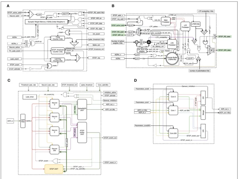
The hardware platform we are using here for Stochastic 1-bit weights STDP allows for on-line unsupervised learning of the FE layer, with simultaneous on-line supervised STDP-based classifier learning (Yousefzadeh et al., 2017). This digital hardware has been designed using standard Hardware Description Language (HDL) and is implemented on a Spartan-6 based FPGA (XC6SLX150T-3) custom platform.Figure 3shows the hardware setup used8.
Two main blocks have been developed for the hardware implementation on digital FPGAs: aneuron blockand anSTDP unit. The STDP unit can be shared by several neuron blocks, as STDP processing has much lower occurrence. The inhibition mechanism prevents two or more neurons from simultaneously learning a pattern. Therefore, at the most one single neuron will be requesting usage of the STDP unit at a given time. Additionally, by separating firing and STDP thresholds, STDP thresholds are reached with lower frequency than average firing rate. Consequently, the STDP unit will be requested with much less frequency than the neuron updates. Therefore, one single STDP unit can be shared by several neurons. In our hardware implementation, several neurons with one STDP unit form a
neural core. Next we describe each block.
2.6.2.1. Neuron block
Figure 4A shows the structure of a neuron block. The implemented neuron block contains a 1024-bit synaptic RAM to keep the values of up to 1024 binary synapses, three counters (“Firing Counter,” “STDP_threshold Counter,” and “Learning Counter”), some D-type flip-flops (D-FF), three logic comparators, and a few digital gates. The 1024-bit synaptic memory has two independent ports, one is used inside the neuron block (syn_weight) to read synaptic weights and the other one is connected to an STDP bus (STDP_RD_data) for STDP type of operations. When a new spike comes in, signal port “AERin_v” will be activated. “AERin” contains the address of the incoming spike. The corresponding synaptic weight for the incoming spike will be read from the synaptic memory, which requires 3 clock cycles. If the synaptic weight is one, then the state of the neuron should be increased by one, by asserting “count_up.” For the neuron implementation we keep two separate states, each with its own counter, the “Firing Counter” for inference and the “Learning Counter” for learning. The “STDP threshold Counter” stores the threshold for the STDP events. After each learning/STDP process, the value of the STDP threshold is increased by one. The values of the “Learning Counter” and the “Firing Counter” are constantly compared with their corresponding threshold values to generate an STDP event (“STDP_req”) or an output event/spike (Spike_out), respectively. The neuron states are reset to zero if they exceed the threshold or an external reset event inhibits them because of lateral inhibition. When a neuron asserts the “STDP_req” signal, the
FIGURE 3 |Hardware setup for demonstration of on-line real-time Stochastic Binary-Weights STDP learning. This setup contains an Event-Player (USBAER board) (Serrano-Gotarredona et al., 2009) to play back recorded AER events with precise timing, an AER-NODE board (Iakymchuk et al., 2014) which contains the Spartan-6 (XC6SLX150T-3) FPGA and a computer interfacing board (USBAERmini2) (Serrano-Gotarredona et al., 2009) to send the output AER events along with their time-stamps to a computer through USB. The computer uses jAER (Delbruck, 2007) to visualize and/or record events in real time displaying them as sequences of frames on a monitor screen.
external STDP unit will access the synaptic memory (through “STDP_active_addr”) to perform the learning process. Since the STDP unit is shared by multiple neurons, neurons are connected to a shared bus, which we callSTDP_BUS(seeFigure 4C), made of signals {STDP_active_addr, STDP_RD_add, STDP_WR_en, STDP_WR_data and STDP_RD_data}.Neuron_addr is unique for each neuron. When the STDP unit wants to access a neuron’s weight, it will put the address of the neuron in the
STDP_active_addr line. Each neuron can process one input spike per clock cycle, because the 3-cycle reading from synaptic memory is pipelined.
In a Spartan-6 FPGA (XC6SLX150T), each neuron occupies only 56 slices (out of 23 K) and it can be clocked at up to 300 MHz [therefore, each neuron can process up to 300 Meps (mega events per second)]9. This allows to implement more than 400 physical neurons and 400,000 synapses in this FPGA without using block-RAMs.
2.6.2.2. STDP unit
The STDP unit is significantly more complex than the neuron block.Figure 4Bshows a detailed block diagram for the STDP unit. This unit contains a circular buffer to memorize the addresses of up to the latest 1024 incoming spikes (which we called “pre-list” or “pre-Buffer” in section 2.2), three processors (Main Processor, LTP Processor, LTD Processor), a 10-bit random number generator (LFSR), four counters (rd_counter,
div_latency_cnt,Cnt_Sum of weights, LTP_cnt+1), a subtracter
9It should be clarified that reducing the clock frequency helps to reduce the number of of slices. For lower speeds, fewer resources are required, in general.
logic block, a ×1024 multiplier block (implemented as a 10-bit shift), a divider block, three logic comparators, three multiplexers, a number of D-FF registers, and digital gates.
Parameter “number of potentiation” indicates how many events in the circular pre-Buffer will be actually used (“number of potentiation”≤1024). This information is used for the LTP (long term potentiation) process. The main processor acts as a general manager. Activation of signal STDP_addr_v means that the STDP unit has received an STDP request. In this case, if the main processor is ready to process a new request, it puts the address of the selected neuron on theSTDP_active_addr line. Then it asserts the start signal for the LTP processor. After finishing the LTP process, it will assert the start signal for the LTD (long term depression) processor. The first step of the STDP process is LTP. In this step, the LTP processor controls theSTDP BUS
of the selected neuron. It reads the addresses of the most recent spikes that are stored in the circular buffer and puts them on the
STDP_RD_addrbus. Then, after reading the synaptic weight, the value needs to be potentiated with a pre-defined probability. In this case, a 16-bit LFSR generates a pseudo-random number. It compares 10 (out of 16) bits of this random number with the LTP probability value, and if the random number is smaller than the probability value, the synaptic weight will be potentiated to “1” if it was “0” before. This process repeats until the number of LTP actions becomes equal to parameter “number of potentiation.” Each potentiation can be done in one clock cycle but there is a 3 clock cycle latency for reading from the circular buffer and the same for reading from the synaptic memory of the neuron. One clock cycle latency is also added for the STDP_WR_data
FIGURE 4 | (A)Neuron block schematics.(B)STDP unit schematics.(C)Neural core schematics.(D)Multi-core configuration.
process requires 7+num_potentiation clock cycles, which in the worst case is 1024+7=1031 clock cycles. After the LTP process, the LTD process starts to depress some weights randomly and normalizes the number of active weights in a synaptic memory. The LTD processor first reads all the synaptic weights of the selected neuron to compute the sum of the weights and calculates the depression probability. This will take 1024+3 clock cycles. Then a subtracter logic block calculates the difference between the number of actual active weights and the number of expected active weights (1W). After this, a logic 10 bit shift multiplies
1Wby 210 to scale it. Then a divider logic block calculates the normalized LTD probability with the following formula
LTD Probability= 1024×1W Wsum
(1)
whereWsumis the number of actual active weights. This process
requires 25 clock cycles because the divider logic is very small and it is a slow serial divider. Since only one division is needed for the whole STDP process, it is efficient to use a slow and
small divider. After calculating the LTD probability, the LTD processor reads again all the synaptic weights, one by one, and depresses them using this probability. This step requires 1024+7 clock cycles. Therefore, in total, the LTD process requires 1024+3+25+1024+7=2083 clock cycles.
At the end of the STDP process, all the pointers in the circular buffer will be reset. This implements pre-list flushing. In HW, lateral inhibition is very strong by directly resetting all neurons within the same population sharing the same STDP UNIT. Consequently, it does not make sense to keep the old events in the circular buffer for future STDP. This simplifies dramatically the HW. Otherwise, if lateral inhibition would have been soft, we may think of not flushing the pre-list. But this would require to add the following complication: since the STDP process is much slower than the neuron updates, while an STDP update is running, new incoming events should not be included in the circular buffer before the running STDP process is finished, requiring the introduction of an intermediate buffer whose content would be transferred to the circular buffer once the STDP update process is concluded.
The proposed design implemented in Spartan-6 (XC6SLX150T-3) consumes 120 slices (out of 23k), and it can operate at a clock frequency of up to 200 MHz10. The exact time of the STDP process depends on one parameter (number of potentiation), which in the worst case needs 2083+1031=3114 clock cycles, or 15µs.
As a practical consideration, a VLSI design needs a hierarchical approach to be extensible and reusable. Here we implemented a Neural-Core as a single processing core that contains an arbitrary number of 256 neurons and one STDP unit.
Figure 4C shows the block diagram of this Neural-Core. Each core contains two arbiters. One arbiter (“STDP arbiter UNIT”) is in charge of handling STDP requests from the neurons, while the other arbiter (“Spike2AER UNIT”) is in charge of handling the output spikes produced by the neurons. Since the number of neurons per core can be large, the use of the shared bus (“STDP_BUS”) reduces long-distance wiring resources. There are only 2 signals (1-bit each) that need to be routed separately for each neuron: “Spike_out” and “STDP_req.” An AER filter is implemented at the “AERin” input to filter out all input spikes whose destination is not the present Neural Core. The Neural Core can have any arbitrary number of neuron units, as long as their output activity does not saturate the shared “STDP UNIT.”
2.6.2.3. Multi-core configuration
Figure 4D illustrates an arrangement of a multi-core configuration for the case of a one-layer fully connected neural network with an arbitrary number of 256 cores (65 k neurons). This can be one layer of a deep neural network. In this case each core can have its own parameters.
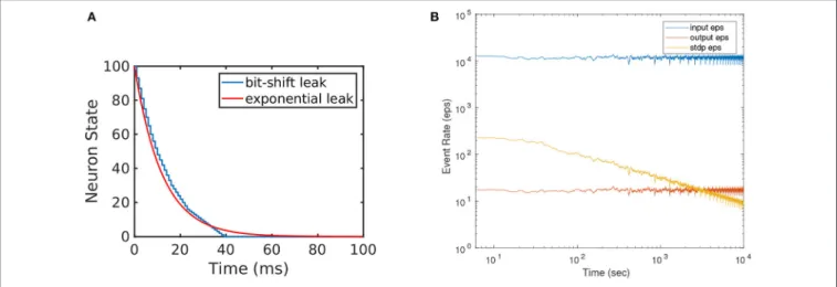
The efficiency of the presented hardware implementation comes from the simplicity of the neuron model, of the learning rule, and from using 1-bit synaptic weights. We approximate the exponential leak by a simplified piece-wise-linear leak, by using a bit-wise shift mechanism for leakage11(Yousefzadeh et al., 2017). Figure 5A shows the exact exponential leak (with 12 ms time constant), together with the approximated piece-wise-linear one. Initially, a large number is subtracted every time (fast linear leak), but this number is divided by a power of 2 at some point, reducing the slope of the linear leak. Additionally, the simplicity of the order-based STDP learning rule avoids keeping track of time, saving on-chip memory. For a comparison,
Rice et al. (2009)implemented 25 physical Izhikevich neurons (without any learning scheme) in a Virtex4 FPGA, consuming 79% of total resources (more than 2 k slices per each physical neuron) which is around 40 times more than the resources used for the simple neurons used in this work. Cassidy et al. (2007)presented an FPGA design with 32 LIF neurons and 128 8-bit synaptic connections per neuron which are equipped with conventional time-based STDP learning and operates at 50 MHz clock frequency. Their design consumed 7454 slices of Xilinx
10Reducing clock frequency helps reducing the number of slices.
11Note that for the hardware implementation we have used a more sophisticated leak than for the software implementations. In software we used plain linear leak, while in hardware we are approximating an exponential leak. However, the circuit implementation is simpler: the plain linear leak requires one subtracter and one comparator, while the piece-wise-linear exponential approximation requires one subtracter and bit-shifting.
Spartan-3 FPGA and 20 KB of block RAMs while our proposed design with 256 neurons (including STDP unit and clocking at 100MHz) consumed 6210 slices and no block RAMs12. This means that by using 1-bit weights, we were able to integrate more than 8 times smaller neurons with 8 times more connections per neuron, while having almost identical resource consumption.
3. RESULTS
This section describes three learning experiments performed on three different data sets, using either the MegaSim software platform, the FPGA hardware platform, or both. The first one is an experiment on the unsupervised development of simple orientation selectivity fields replicating biological experiments (Bienenstock et al., 1982). These biological experiments demonstrate the development of stimulus orientation selectivity in the primary visual cortex. To replicate this biological experiment no classifier layer was used, and results were obtained for both the MegaSim software platform and the hardware FPGA platform. The second experiment is a poker card symbol classification experiment using real DVS recordings. We used the so called “Slow Poker DVS” data set (Soto, 2017), which consists of relatively long recordings of hand held printed poker symbols, that allowed for a reasonable large training set. This experiment required a classification layer, and we used both, the high performance and the simple STDP-based ones. Results were obtained for the MegaSim and the FPGA platforms. The third experiment is an MNIST handwritten digits (LeCun et al., 1998) recognition experiment. For this experiment we required the high performance classifier, as the simple classifier provided poor performance for such a complex data set. Results were only obtained for the MegaSim platform, because the high performance classifier cannot be trained on-line by the hardware. In the following we show details of the different experiments and corresponding results.
3.1. Development of Orientation Selectivity
This experiment is based on the work presented inBienenstock et al. (1982) and was used to experimentally demonstrate the development of stimulus selectivity in the primary sensory cortex. The topology of this neural network was shown in
Figure 2D. It consists of two layers, one input layer of size 32×32, which is fully connected to a FE layer of 4 neurons. The synthetic stimulus used for the training is a bar presented in 4 different orientations, rotated by 45o. The bar is 8 pixels thick, and 24
pixels in length, while each pixel has a random intensity value between 0.8 and 1.0. The pixels are then converted to Poisson spike-trains with a rate proportional to the intensity of each individual pixel. This is a common technique for converting static images to synthetic spike-trains (O’Connor et al., 2013; Querlioz et al., 2013; Diehl et al., 2015; Diehl and Cook, 2015; Galluppi et al., 2015; Stromatias et al., 2017). The four different orientations used for the training can be seen in Figure 6A. During training, each bar is presented in one of the four random
12Spartan-3 FPGA is older than Spartan-6 and, by our experience, a similar design may take around 10% fewer slices in Spartan-6 in comparison to Spartan-3.
FIGURE 5 | (A)Illustration of the implemented efficient leakage mechanism by using bitwise shift. This approximates exponential leakage in LIF neurons.(B)Event rate of input, output, and STDP output during STDP learning. Horizontal axis (time) is shown in log scale to visualize the exponential decay in STDP output events. One training set trial is about 400 s.
orientations, with an inter-symbol time equal to Tleak, thus
allowing all neurons to leak to their resting state.
The parameters of the fully connected neural population are summarized inTable 1top, while the STDP parameters can be seen inTable 1bottom.Figure 6Btop shows the initial random 1-bit weights before learning, andFigure 6Bbottom shows the final 1-bit weights after 400 training epochs. It can be seen that by the end of the training each neuron has developed a receptive field specific to a particular orientation. The purpose of the post-learning test is to demonstrate that each neuron has learned to respond maximally to a preferred orientation. For this, we disabled the (a) plasticity, (b) dynamic thresholds, and (c) internal (inhibition) reset mechanism. Neuron thresholds are kept at their final training values (which isxthmax).
This experiment has been performed both on the MegaSim and on the FPGA platforms, presenting identical results.
Figure 6Bshows the firing frequencies of the four neurons as a function of input stimulus bar orientation, in steps of 10◦. As the
bar rotates, the neuron tuned to the closest orientation provides higher firing frequency, as happens in biology (Bienenstock et al., 1982) and other similar experiments (Moore and Freeman, 2012; Jeyabalaratnam et al., 2013; Galluppi et al., 2015). For the rest of the paper, in the remaining experiments, we will consider the spike count of the output neurons, for a given input stimulus, as the quantity determining the readout of the neurons.
In the FPGA, we implemented four physical neurons and one STDP UNIT. The complete circuit power consumption was 142 mW when operated at 100 MHz clock frequency. This design occupied only 1% of the FPGA slices. A video demonstration of the FPGA version of this experiment can be seen in (Yousefzadeh, 2017b).
3.2. Recognition of DVS-Recorded Poker
Card Symbols
A very high speed DVS recorded poker symbol data set was released in the past (Serrano-Gotarredona and Linares-Barranco,
2015). However, this data set contained too few training samples for proper STDP learning and classifier training. To perform more robust poker symbol recognition training, a new data set was recorded called “Slow-Poker-DVS,” in which paper printed poker symbols were hand held in front of a DVS and moved slowly to induce motion events (Soto, 2017). This data set consists of four 3 min recordings, each recording for a different poker symbol. The recordings use the full 128×128 DVS resolution. For each recording, we extracted slices with a fixed number of events per slice, rather than with a fixed time window. More specifically, we used slices of sizes 10, 30, and 50 kilo events per slice (kesl). Therefore, we had three different data sets for training and testing, depending on the chosen kesl. Each slice is not like a static frame, but rather like a moving video, and a few neurons may fire and learn during each slice. For finding the optimal learning hyper parameters such asWsum,xthmax,STDP Buffer Size,
andPLTP, we used a validation set to avoid over-fitting the testing
set (Nowotny, 2014).
The number of samples of the training and testing set varies depending on the number of kesl. For 10 kesl, we had 779 samples in the training set (of which 138 samples are used for the validation set) and 192 samples in the test set. For 30 kesl we had 259 samples in the training set (of which 45 are used as the validation set) and 64 samples in the test set. Finally, for 50 kesl we had 155 samples in the training set (of which 26 samples are used for the validation set) and 37 samples in the test set. For each experiment the hyper parameters that generated the highest score on the validation set were used to train on the full training set and report the final score as CA on the testing set.
3.2.1. Software Results
For each data set we trained the SNN with different number of neurons in the feature extraction layer, the layer that will learn with 1-bit weights. The number of neurons we tried for this layer were {200, 400, and 800}. The experiments were executed by applying aPLTPof 20 and 80%, a number of active synapses per
FIGURE 6 | (A)The input pattern used for the orientation selectivity experiment. During the experiments the bar is presented in random order.(B) The initial and final 1-bit weights for the development of orientation selectivity experiment.(C)Orientation tuning curves obtained by rotating a horizontal bar counter clockwise with a step size of 10◦C.
receptive fieldWsumof {16, 32, 128}, andxthmaxof {40, 60}. The
STDP buffer size was kept fixed at 250 events to reduce simulation time.
In order to find the optimal hyper parameters, we used the validation set of each data set. For each data set, each training set is presented once with stochastic STDP learning activated. Then, the hyper parameters that resulted in the highest classification accuracy (CA) on the validation set were chosen to train with the full training set, and after this the classifier (output layer) was trained. The final score is reported using the testing set of each data set. Table 2 gathers the hyper parameters that were investigated for the Slow-Poker-DVS experiments, when using
TABLE 1 |Neural and STDP parameters for the development of orientation selectivity experiment.
Parameters Values Description
Neural parameters
population_size 4 Population size
pre_size 1024 presynaptic population size
xth 10 Initial Neuron Threshold
xthmax 100 Maximum allowed dynamic threshold
STDP parameters
STDP buffer size 250 Total size of the event buffer
PLTP 80% Probability for LTP
Wsum 180 Sum of active synapses per neuron
TABLE 2 |STDP hyper parameters investigated for the MNIST classification task.
Parameter Values Description
STDP buffer size [250, 500] STDP event buffer size
Wsum [16, 32, 128, 256] Number of active synapses per neuron
PLTP [80%, 20%] Potentiation probability
xthmax [40, 60, 80] Maximum allowed threshold during
STDP learning
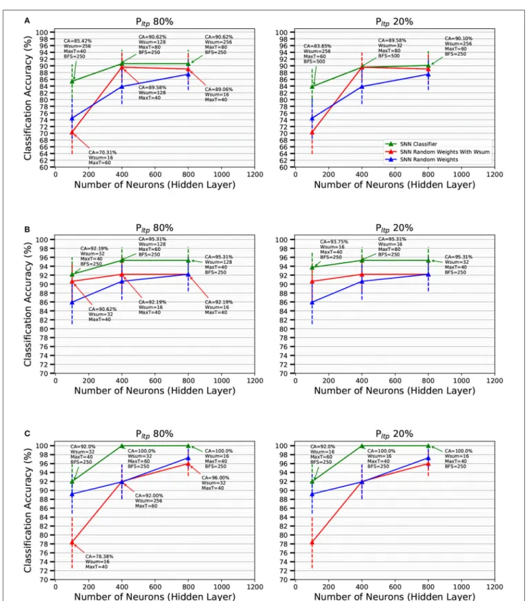
the MegaSim platform with the high performance event-driven classifier (Stromatias et al., 2017). The corresponding results are summarized inFigure 7. The green line represents CA on the corresponding testing set as a function of the number of neurons in the 1-bit weights feature extraction layer. Figures 7A–C
correspond to data sets created using 10, 30, and 50 kesl, respectively. It can be seen that there is no significant difference between processing most of the incoming STDP updates (PLTP
= 80%) or just a portion of them (PLTP = 20%). Although CA
improves with more neurons in the feature extraction layer, the number of kesl has a more significant effect on the CA. Along with the CA,Figure 7 presents the confidence interval (CI) for each result with a vertical bar. The CI is calculated for a confidence level of 0.99 and assuming that the test samples are statistically independent (Nowotny, 2014). The confidence intervals show the expected CA depending on the test set size. The confidence intervals of the mean test error are computed using the following expression (Nowotny, 2014)
ˆ µ±z∗( s ˆ µ(1− ˆµ) NT ) (2)
whereµˆ is the estimated test error,NT is the test set size, and
z∗depends on the level of confidence. For 0.99 confidence level,
z∗is 2.578. Note that the resulting range of the CI is quite wide because the data set used is not very large. Furthermore, with the increase of kesl, the number of samples of the data set and the test set becomes smaller and the CI increases.
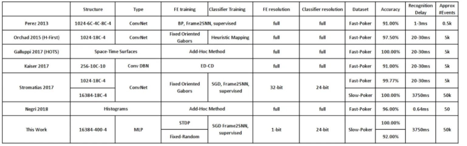
The “Slow-Poker-DVS” data set was used before with the same high performance classifier, but using a feature extraction layer of 18 pre-programmed non-plastic oriented Gabor filters
FIGURE 7 |Classification Accuracy (CA) of the SNNs on the Slow-Poker-DVS data set as a function of the number of neurons in the FE layer for aPLTPof 80 and
20%, shown as the green solid line, for(A)10 kesl,(B)30 kesl, and(C)50 kesl. The text at each data point presents the hyper parameters that yielded the best CA on the validation set. The blue solid lines show the CA for random fixed 1-bit weights with no STDP learning in the FE layer, while the red lines show the CA for random fixed 1-bit weights with fixedWsumapplied to restrict the number of active synapses per neuron.PLTPis not applicable for the blue and red solid lines; they are
duplicated in each pair of subplots for viewing convenience. The error bars denote the confidence and are calculated for a confidence level of 0.99 and assuming that the test samples are statistically independent (Nowotny, 2014).
(Stromatias et al., 2017), obtaining a CA of 99.7%. Slices were extracted using 100 ms time windows, generating a total of 6751 samples for the full data set. Here we decided to be independent of the time variable and create slices using number of events. However, the large number of events required for a good CA, results in a reduced number of samples in the data set, which increases the CI for each result. Using fixed time slices we obtained 99.7% CA (Stromatias et al., 2017). On the other hand, here the data set got reduced drastically, but we achieved even better CA, despite using 1-bit weights, a smaller network size, and training the feature extraction layer in an unsupervised manner.
In order to “measure” the effectiveness of the STDP-trained FE layer, we compare with the case of using pure random 1-bit weights in the FE layer. It is well-known that a sufficiently large FE layer with random weights followed by a high-performance classifier yields highly competitive accuracies (Huang et al., 2006). Here we want to see if stochastic STDP learning with 1-bit weights improves with respect to pure random 1-bit weights, using the same FE layer size. The results are shown inFigure 7with blue and red traces. Blue traces correspond to generating random 1-bit weights without any restriction. Red traces correspond to the same, but with the restriction of keeping the sum of 1-bit weights (connecting to one destination neuron) equal toWsum. We can see there is a systematic benefit when
using stochastic STDP with respect to random weights. The benefit tends to be more for smaller number of neurons in the FE layer.
3.2.2. Hardware Results
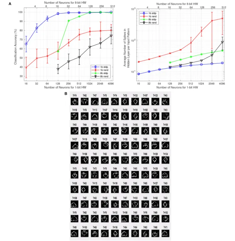
In addition to the MegaSim based experiments with the high performance classifier, we also performed some tests using the digital hardware FPGA platform with the simplified event-driven classifier. The FPGA platform results shown inFigure 8A(trace “1b stdp”) correspond to the 10kesl data set, with input events sub-sampled to 32 × 32 pixel resolution. From each original recording, we used the first 1.6 million events, which resulted in 160 samples per symbol. From these, 80% randomly picked samples were used for the training set and the remaining 20% for the test set. We set up a network with a 32×32 input layer which connects to a feature extraction (FE) layer withNneurons in a fully connected manner. The 32×32×N 1-bit synaptic weights were trained on-line using the proposed stochastic STDP 1-bit rule withWsum = 100. TheNneurons are connected to a
simple STDP-type classifier (as presented before in section 2.5) with 4 output neurons, and trained accordingly (Yousefzadeh et al., 2017). This classifier is implemented in hardware and is trained on-line along with the stochastic STDP neurons. We performed tests using different numbers of neurons N for the FE layer. Also, for comparison purposes, we repeated the same process but without STDP FE learning. Instead, the receptive fields of the N FE neurons were randomly set to 1-bit values, while keepingWsum = 100.Figure 8A(trace “1b rand”) shows
the results when setting the event buffer size to 90 and the probability of potentiation to PLTP = 30%. The bottom axes
in Figure 8A indicate N, the number of neurons in the FE hidden layer. Figure 8A(left) indicates the CA obtained after stochastic STDP learning and classifier training, andFigure 8A
(right) indicates the average number of FE hidden layer spikes per pattern presentation for the full test set. We can see that when using the proposed stochastic STDP FE layer learning, the classifier can learn with up to 100% accuracy withN = 256, while generating much less events. However, when the FE weights are set randomly, the classifier is not able to achieve such high accuracy.Figure 8B shows the stochastic-STDP learned FE 1-bit weights for13 N = 100. For these results, we kept for allN
the same STDP buffer size (90),Wsum (100), and PLTP (30%).
However, the inference threshold was automatically adjusted to have an acceptable activity for classification. In general, a higher activity should lead to improved accuracy as there is more information. However, we can see that for the STDP FE layer, higher accuracy is achieved with lower neural activity (and consequently lower power consumption), which means that extracted features are more efficient and representative. For this experiment, with 256 physical neurons and one STDP UNIT, the FPGA consumed 333 mW when operating at 100 MHz clock frequency. Such design occupied 27% of our FPGA slices.
3.2.3. Trading off Bit-Resolution for Number of Neurons While Maintaining Similar Hardware Resources
An interesting question one may ask is what if, for the same hardware resources, we increase bit-precision while reducing number of neurons and synapses. Will we gain in CA or power consumption? Changing bit-precision affects all circuitry: synapses, neurons, as well as all computing and communication circuitry. Although a full detailed study is out of the scope of the present paper, we can quickly analyze the case for an 8-bit system, using both STDP or fixed random 8-bit weights. For example, as reported by Cassidy (Cassidy et al., 2007), they implemented an STDP 8-bit system using very similar hardware resources than our 1-bit STDP implementation (seeTable 5). The number of synapses and neurons they were able to fit was exactly 1/8 the ones we have used. Therefore, as an approximate rule of thumb, we can suggest that increasing/decreasing bit resolution by a given number, decreases/increases both the number of synapses and neurons in the hidden layer by the same number. This observation is actually quite intuitive when implementing a hidden layer withNiinputs,Nhhidden neurons, andNsyn =
Ni×Nhsynapses. IfRhrepresents the hardware resources for the
hidden layer neurons,Rsynthe ones for the synapses, andRovthe
ones for the rest of overhead (shared) circuitry, then
Rsyn = αsyn×Ni×Nh×nb (3)
Rh = αh×Nh×nb (4)
Rov = αov×nb (5)
wherenbis the number of bits, andαsyn,αh, andαovare some
proportionality constants. AssumingRov << Rsyn +Rh, then
we can see that the productNh×nbmust be kept constant for
equal hardware resources. Consequently, we may assume that if we change bit resolution from 1-bit to 8-bit, we must divide
13A video showing the evolution of the 1-bit weights during stochastic STDP learning can be seen in (Yousefzadeh, 2017a).
FIGURE 8 | (A)CA (left) and output neuron spikes (right) for STDP trained FE weights and random FE weights. The figure compares 1-bit hardware (bottom axes) with 8-bit hardware (top axes). Bottom and top axes are aligned for similar hardware resources consumption. Blue circles: 1-bit HW with STDP. Red exes: 1-bit HW with fixed random weights. Green asteriscs: 8-bit HW with STDP. Black triangles: 8-bit HW with fixed random weights.(B)Stochastic-STDP learned weights on the FPGA hardware platform for buffer size 90 andPLTP=30%. The number on top of each receptive field indicates the final neuron thresholdxthafter learning has concluded.
Nhby 8. InFigure 8Awe show CA (left) and Average Number
of Hidden Layer Spikes per Input Pattern (right) as a function of the number of neurons for different implementations. The horizontal axes have been separated into two: the bottom one for 1-bit hardware and the top one for 8-bit hardware. This way,
hardware of similar resources is aligned vertically. For example, a 1-bit implementation with 256 hidden layer neurons is aligned vertically with an 8-bit implementation of 32 neurons, because both consume similar hardware resources. Vertical segments at each data point, represents the max/min spread when repeating
the training over 10 full trials. For the case of 8-bit STDP training there are no vertical segments, because in this case STDP is deterministic: STDP applies small changes every time without generating random numbers in the process.
FromFigure 8Awe can make some interesting observations. (a) The 1-bit hardware with STDP provides, for given hardware resources, the highest CA and the minimum number of spikes in the hidden layer. Note that the number of spikes is directly proportional to power consumption in an event-driven system, because computation and information communication is performed at a per-event basis. Also note that computing events in 1-bit hardware consumes less energy than with 8-bit hardware (although, this is not reflected inFigure 8A). (b) CA seems to depend mainly on the number of neurons, while depending very little on the bit representation used. In Figure 8A left, when shifting the 8-bit HW curves to align exactly the number of neurons, the resulting curves almost overlap. (c) For the fixed random weights (both 1-bit and 8-bit) there is a sudden increase in number of events as hidden layer neurons increase, while for the STDP cases the tendency seems to be to settle smoothly. Please note that none of these observations is conclusive, and should not be extrapolated to more general cases before a more careful and systematic study is performed.
3.2.4. Bandwidth Limitations of STDP Hardware During Learning
From section 2.6.2 we can see that the hardware resource usage of the STDP unit within one 256-neuron core (see Figure 4C) is about 2-3 neurons, or equivalently, about 1% of the neural core. Therefore, from the hardware resources point of view, the difference between a 1-bit STDP hardware and a 1-bit fixed random weights hardware is negligible. On the other hand, the biggest advantage of the fixed random weights option is that it does not require training. From the bandwidth point of view, the STDP version has some bandwidth limitations during learning. For inference, both versions have identical bandwidth because the neuron hardware is the same. Neurons can process one event per clock cycle. Therefore, for the 100 MHz clock frequency implementation (see section 3.2.2) the maximum input event throughput is 100 Meps. Additionally, the maximum output event throughput cannot exceed 100Meps, for the same reason.
However, the STDP version needs to be trained and, during training, the STDP unit imposes some additional bandwidth limitation, which can be reached under some circumstances. In our example implementation, the STDP unit is shared by 256 neurons, and is triggered every time one of the 256 neurons generates an STDP output event. Each STDP output event also resets the STDP counters of the rest of neurons, thus helping to make the STDP output activity sparse. As mentioned in section 3.2.2, the STDP process needs “2090 + buffer size” clock cycles. In our example implementation “buffer size=90,” thus requiring 2180 clock cycles per output event (21.8µsat 100 MHz clock frequency). Therefore, the STDP unit would saturate at an STDP output event rate of 45.87 keps. Note that saturating the STDP unit is not a dramatic problem: while saturated, all STDP output events will be ignored and training would require more time.Figure 5Bshows, as an illustration for the 256-neuron
hidden FE layer case, the instantaneous event rates for the input flow (average around 12 keps), for the output flow (average around 18 eps), and for the output STDP events. We can see that STDP output event rate starts with a maximum of about 220 eps and decreases exponentially with time as learning progresses. Consequently, one could accelerate the input event rate by a factor 45.87k/220=208 before saturating the STDP unit during the initial learning phase, which would result in an input event rate of 2.5 Meps. Alternatively, if one wants to avoid STDP unit saturation, it is possible to add more STDP units and have them shared by less neurons.
3.3. Recognition on the MNIST Data Set
The MNIST data set (LeCun et al., 1998) consists of 70,000 samples of handwritten digits from 0 to 9, of which 60,000 are used for training and 10,000 for testing. Each sample is a 28×28 gray-scale image with maximum intensity value of 255. We converted the MNIST data set from static images to Poisson-distributed spike-trains with a rate proportional to the intensity of each pixel, while all firing rates are scaled in order to keep the total firing rate of the population constant (O’Connor et al., 2013; Stromatias et al., 2017, 2015).
MNIST dataset learning was only possible when using the high performance classifier for the output layer. Otherwise, accuracy results were very poor. Consequently, here we only focus on software platform results with the high-performance classifier. During STDP learning we presented one sample at a time, 1000 spikes per training sample, with an inter-symbol-time (IST) identical to the linear leakage of the spiking neurons. This way the leakage acts as a natural way to reset the internal states of the neurons before presenting a new training sample.
We first train the FE layer using the topology shown in
Figure 2D. Stochastic STDP learning stops when all training samples are presented once. Training was repeated for different number of neurons in the FE layer. For the output layer we used the high performance event-driven classifier described in section 2.5. For finding the optimal learning hyper parameters such asWsum, xthmax, STDP Buffer Size, and PLTP, we used a
validation set to avoid over-fitting the testing set (Nowotny, 2014). We split the original 60, 000 samples of the full training set into a training set of 50, 000 samples and used the remaining 10, 000 samples as the validation set. For each experiment the hyper parameters that generated the highest score on the validation set were used to train on the full 60, 000 samples training set and we report the final score as CA on the MNIST testing set.
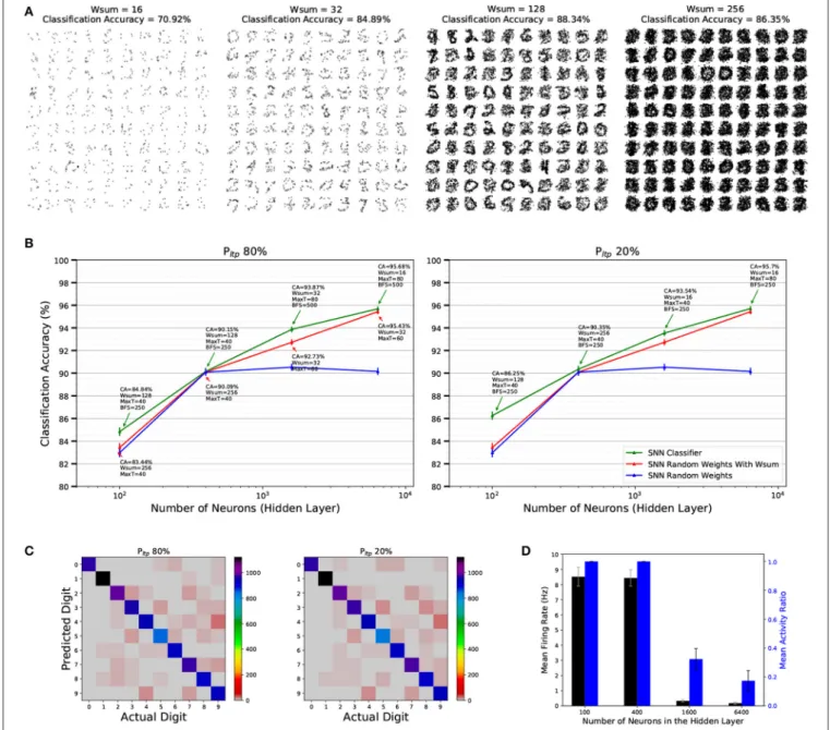
We trained a series of SNNs with varying number of neurons in the stochastic STDP FE layer. The number of neurons were {100, 400, 1600, 6400}, as in (Diehl and Cook, 2015) to allow for a direct comparison.Table 2shows the STDP hyper parameters that were investigated.Figure 9A shows the effect that Wsum
has on the learned weights of a population of 100 neurons. Results are summarized inFigure 9B. The green solid line in
Figure 9Brepresents CA on the MNIST testing set as a function of the number of neurons in the FE layer, along with the hyper parameters that generated the highest CA on the validation set. ForPLTP = 80% the SNNs achieve the following classification
FIGURE 9 | (A)Effect ofWsumStochastic-STDP meta parameter on the 1-bit weights (receptive fields) and the classification accuracy (CA) of a population of 100
neurons trained on the MNIST data set. Weights are reshaped from 784 to 28×28.(B)Classification Accuracy (CA) of the SNNs on the MNIST testing set as a function of the number of neurons in the FE layer for aPLTPof 80 and 20%, shown as the green solid line. The text at each data point presents the hyper parameters
that yielded the best CA on the validation set. The blue solid line shows the CA for random fixed 1-bit weights with no STDP learning in the FE layer, while the red line shows the CA for random fixed 1-bit weights with fixedWsumapplied to restrict the number of active synapses per neuron. Error bars denote the confidence and are
calculated for a confidence level of 0.99 and assuming that the test samples are statistically independent (Nowotny, 2014).(C)The confusion matrix on the 10, 000 MNIST testing set digits for a FE layer of 6400 spiking neurons when applied STDP learning with a PLTPof 80 and 20% respectively. Values on the diagonal represent
correct classifications.(D)Mean neuron firing rate and mean activity ratio of the FE layer for all 10, 000 samples of the validation set and for 4 different population sizes.
accuracies for populations of 100, 400, 1600, and 6400 neurons in the FE layer: 84.84, 90.15, 93.87, and 95.68%, while for aPLTP =
20% CA is 86.25, 90.35, 93.54, 95.7%. These results demonstrate that there is no significant difference between processing the majority of incoming STDP weight updates or just a fraction of them. Another visible trend from Figure 9B is that, as the number of neurons in the FE layer increases, configurations with smallerWsum(less active synapses per neuron) yield higher
classification accuracies, while for smaller population sizes larger
Wsumresult in higher CA.Figure 9Bpresents the CA along with
the confidence intervals (CI).
Figure 9Cshows the confusion matrix of the MNIST test set for the 6,400 neurons case for aPLTP of 80 and 20%. Values
on the diagonal represent correct classifications. While executing simulations with the validation set we discovered that the activity of the FE layer after stochastic STDP learning for the larger