Tools for label-free peptide quantification
Sven Nahnsen1, Chris Bielow2, Knut Reinert2, and Oliver Kohlbacher1 1 Center for Bioinformatics, Center for Quantitative Biology,
and Department of Computer Science, University of T¨ubingen, Germany
2 Institute of Computer Science, Freie Universit¨at, Berlin, Germany
Corresponding author:
Prof. Dr. Oliver Kohlbacher,
Center for Bioinformatics, University of T¨ubingen, Sand 14, 72076 T¨ubingen, Germany.
Tel.: +49 7071 29 7 04 58; Fax: +49 7071 29 51 52;
e-mail: [email protected]
Running title: Computational tools for peptide quantification
Abbreviations
MS/MS: Tandem mass spectrometry LTQ: Linear trap quadrupole
LCQ: Liquid chromatography quadrupole SC: Spectral Counting
TOPP: The OpenMS proteomics pipeline ppm: parts per million
Abstract
The increasing scale and complexity of quantitative proteomics studies complicates the subsequent analysis of the acquired data. Untargeted label-free quantification, either based on feature intensities or on spectral counting, is a method that scales particularly well with respect to the number of sam-ples. It is thus an excellent alternative to labeling techniques. In order to profit from this scalability, however, data analysis has to cope with large amounts of data, process them automatically, and do a thorough statistical analysis in order to achieve reliable results.
We review the state of the art with respect to computational tools for label-free quantification in untargeted proteomics. The two fundamental approaches are feature-based quantification, relying on the summed-up mass spectrometric intensity of peptides, and spectral counting, which relies on the number of MS/MS spectra acquired for a certain protein. We review the current algorith-mic approaches underlying some widely used software packages and briefly discuss the statistical strategies required to analyze the data.
1
Introduction
Over the last decades mass spectrometry has become the analytical method of choice in most pro-teomics studies (e.g. [1, 2, 3, 4]). A standard mass spectrometric workflow allows for both, protein identification and protein quantification [5] in some form. For a long time, the technology has been mainly used for a qualitative assessment of protein mixtures, namely to assess whether a specific protein is in the sample or not. However, for the majority of interesting research questions, espe-cially in the field of systems biology, this binary information (present or not) is not sufficient [6]. The necessity of more detailed information on protein expression levels drives the field of
quantita-tive proteomics [7, 8], which also enables to integrate proteomics data with other data sources and allows network-centered studies, as reviewed in [9]. Recent studies show that mass spectrometry-based quantitative proteomics experiments can provide quantitative information (relative or abso-lute) for large parts, if not the entire set of expressed proteins [10, 11, 12].
Since the ICAT (isotope-coded affinity taq) protocol was first published in 1999 [13], numerous la-beling strategies found their way into the field of quantitative proteomics [14]. These include ICPL (Isotope-coded protein label) [15], metabolic labeling [16, 17] or isobaric taqs [18, 19]. A compre-hensive overview of different quantification strategies can be found in [20, 21]. Due to shortcom-ings of labeling strategies, label-free methods are increasingly gaining the interest of proteomics researchers [22, 23]. In label-free quantification no label is introduced to either of the samples. All samples are analyzed in separate LC-MS experiments and the individual peptide properties are then compared between the individual measurements. Regardless of the quantification strategy, compu-tational approaches for data analyses have become the critical final step of the proteomics workflow. An overview of extisting computational approaches in proteomics is provided by [24, 25] The com-putational label-free quantification workflow in visualized in Fig. 1.
Comparing peptide quantities using mass spectrometry remains a difficult task, since mass spec-trometers have different response values for different chemical entities, hence a direct comparison of different peptides is not possible. The computational analysis of a label-free quantitative data set consists of several steps that are mainly split in raw data signal processing and quantification. Signal processing steps comprise data reduction procedures, such as baseline removal, denoising and centroiding.
These steps can either be accomplished in modular building blocks or the entire analysis is per-formed in a monolithic analysis software. Recently, it has been shown that it is beneficial to combine
modular blocks from different software tools to aconsensuspipeline [26]. The study also illustrates the diversity of methods that are modularized by different software tools. In another recent publi-cation monolithic software packages have been compared [27]. In this study the authors identify a set of seven metrics: detection sensitivity, detection consistency, intensity consistency, intensity accuracy, detection accuracy, statistical capability, and quantification accuracy. Despite the missing independence of these metrics and the loose reporting of software parameter settings, such compar-ative studies are of great interest to the field of quantitcompar-ative proteomics. A general conclusion from these studies is that the choice of software may to a certain degree impact on the final results of the study.
Absolute quantification of peptides and proteins using intensity-based label-free methods is possible and can achieve excellent accuracy, if standard addition is used. With the help of known concentra-tions, calibration lines can be drawn and absolute protein quantities are directly inferred from these calibration measurements [28]. Furthermore, it has been suggested to predict peptide peak inten-sities and to derive absolute quantities from these predictions [29]. However, the limited accuracy of predictions or the need for peptides of known concentrations limits these approaches to selected proteins/peptides only and prevents its use on a proteome-wide scale.
Spectral counting methods have also been used for the estimation of absolute concentrations on a global scale [30], albeit at drastically reduced accuracy compared to intensity-based methods. In the study, the authors use a mixture of 48 protein with known concentrations and predict the absolute copy number amounts of thousands of proteins based on this mixture. Despite the fact that large, proteome-wide data sets will dilute effects of different peptide detectabilities on the individual pro-tein level, such methods will always be limited in their accuracy of quantification.
[FIGURE 1 SHOULD GO HERE]
The generic nature of label-free quantification is not restricted to any model system and can also be employed to tissue or body fluids [31, 32]. However, the label-free approach is more sensitive to technical deviations between LC-MS runs as information is compared between different measure-ments. Therefore, the reproducibility of the analytical platform is crucial for successful label-free quantification. The recent success of label-free quantification could only be accomplished by signif-icant improvements of algorithms[33, 34, 35, 36]. An increasingly large collection of software tools for label-free proteomics have been published as open source applications or entered the market as commercially available packages.
This review aims at outlining the computational methods that are generally implemented by these software tools. Furthermore, we illustrate strengths and weaknesses of different tools. The review provides an information resource for the broad proteomics audience and will not illustrate all algo-rithmic details of the individual tools.
2
Methods
2.1 The nature of LC-MS/MS data
Quantitative proteomics data from LC-MS and/or LC-MS/MS experiments has typically a large data volume (tens to hundreds of gigabytes per sample are not uncommon) and the data is rather com-plex. Typically, digested proteins, i.e. complex peptide samples, are separated on an LC column, ionized and the resulting MS spectra recorded by a mass spectrometer. For MS/MS experiments,
peptide ions are selected (based on their intensity or through an inclusion list) for fragmentation and fragment ion spectra are recorded. These MS/MS spectra usually form the basis of the identification (which we will not consider here), but can also be used for spectral counting.
Depending on the resolution of the mass analyzer, and since the ionization is a stochastic process, even identical ions will not be measured at the exact same m/z, but rather form a distribution of mea-surements around the true m/z value. This distribution is called a (raw)peakand can be described by a mathematical model (a normal distribution is a good approximation, but not quite sufficient). The process of peak pickingorcentroidingaims at estimating the parameters of the peak model. like for example thecentroid,intensity,width, andskew. Centroiding reduces the raw measurement data to a handful of parameters for each compound and most importantly yields a single value for the m/z of the ion. Thecentroidm/z can be reported as the position of the maximal intensity, or by averaging over m/z (raw data points weighted by intensity). Likewise, theintensity of a peak can be read off as the maximum height from the raw data (the peakapex), or one can compute the area under the curve, i.e., the peak volume. It is important to know whether the data is centroided or not, since some software can handle only one type of input data.
[FIGURE 2 SHOULD GO HERE]
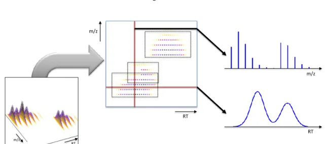
Fig. 1shows a typical data set generated from a biological sample using HPLC-MS and illustrates its multi-dimensional nature. After eluting from the column analytes are continously injected into the mass spectrometer, which records mass spectra (scans) at high speed. Stacking individual spectra yields a three-dimensional dataset, a so-called map. When peptide mass spectrometry is preceded by liquid chromatography fractionation, the observed signal corresponding to a single charge state of a peptide is actually a two-dimensional intensity distribution in retention time and mass-to-charge The data points belonging to this distribution are called afeature(i.e. the two dimensional signal in
Fig. 1).
2.2 Computational methods
Quantification methods can be divided into feature intensity-based methods and spectral counting methods. In the first, one tries to account for all signals corresponding to a specific charged peptide on the MS level, in the second, one tries to infer the expression level of the peptide by the num-ber of MS/MS identifications. Map alignment is especially important for feature intensity-based quantification, while in spectral counting one can use the identification of the peptide to assign cor-responding quantities across maps. Only accurate alignments of maps allow to compare quantitative properties correctly. In the following, we describe the main steps that are necessary for label-free data processing.
2.2.1 Signal processing
Depending on the type of instrument the processing of the raw data can differ. However, there are certain generic steps in signal processing that apply to most instruments. and to both, intensity-based methods and spectral counting. Those arebaseline filtering,noise filtering, centroding, and charge estimation.
In MALDI spectra, and to some extent in ESI spectra, a baseline is apparent which adds up to the signal caused by the analytes. In MALDI spectra the baseline can become dominant in the low
m/z regions and disappears with increasingm/z. It is typically shaped like an exponential decay distribution and can be attributed to matrix material. The baseline leads to poorly resolved peak shapes due to a loss of baseline separation between adjacent peaks. The baseline thus interferes with intensity estimation and has to be removed computationally. Morphological filters like the
Top-hat filter can be for example used for this task.
In addition to the baseline signal, every mass spectrometer suffers from high-frequency noise (elec-tronic noise, usually attributed to the detector, and chemical noise, usually attributed to solvents, buffers, and contaminants) and, thus, peaks expected to be approximately Gaussian shaped might not be convex any longer. This is a potential pitfall for algorithms which rely on local minima to separate isotope peaks. A noise filter will smooth the data by removing high-frequency noise. For example a Savitzky-Golay filter will work well.
Finally, the signal which is baseline corrected and smoothed is subjected to centroiding. The com-putational problem ranges here from almost trivial (e.g. for high resolution spectra) to a fitting of overlapping (skewed) gaussians, for example in the case of highly charged ion trap signals. In gen-eral, this fitting is interweaved with the problem of obtaining the (initially) unknown charge state of a peptide, since the charge state z determines the distance of the isotope peaks, namely 1/z. The resulting model fit can used to analytically determine the peak volume and the height of the peak. Usually the prak volume is taken as the intensity of a centroided peak, since it corresponds directly to the ion count. However, for high resolution spectra the height of the peak (which is easier determined) serves equally well.
2.2.2 Feature-based quantification
Algorithmically, the main steps in feature-based quantification can be divided into signal processing (i), feature-finding (ii) and map alignment (iii). The advent of high resolution mass spectrometers makes the signal processing and peak picking task simpler than on low-resolution instruments. However, the quantification methods are complex and a good quantification remains a challenge.
ions eluting from the LC column. Peptides elute over time from the LC column, get ionized and in-jected into the mass spectrometer. The mass spectrometer takes now measurements in regular, small time intervals thereby sampling the amount of the eluting ion over time, resulting in anelution pro-file. In each measurement, an ion gives rise to a typicalisotope pattern, which is caused by its atomic composition (see Fig. 2 for an example of elution profile and isotope pattern). By integrating over elution profile and isotope pattern, peptide feature intensities can be determined. In general, one can assume that the two-dimensional distribution is a product of two independent distributions. Hence, for the marginal distribution over m/z, a similar reasoning applies as for individual spectra. An automated detection of these features allows their comparison across different experiments. Funda-mental to a quantitative comparison of analytes is the linear correlation of electrospray ionization intensity with ion concentration within a certain dynamic range. Most algorithms try to heuristically determine the extend and intensity of a feature by fitting appropriate distribution models to the data. This is done in areas of high signal intensity (e.g., by working on an intensity sorted list of peaks). The intensity of a feature can then be determined either by using the model parameters, or simply by summing up all peak intensities in the feature region.
2.2.3 Spectral counting
Besides this feature intensity-based quantification method, spectral counting methods are also used for differential quantification. Despite the fact that spectral counting is commonly used to derive quantitative information at the protein level, the differntial quantification of peptides build the fun-dament of this concept. In the following we will discuss spectral counting concepts and illustrate how these concepts perform differential peptide quantification. Spectral counting (SC) in its most simple form counts the number of tandem spectra that are assigned to the same protein. There have been numerous publications using spectral counting for the inference of quantitative information in
label-free shotgun proteomics data. A collection of methods has recently been reviewed [37]. While peptide-spectrum-matchings can be used to infer differential ration of peptides, these methods are also gaining popularity for differential protein quantification. Methods that extend the simple spec-tral counting to differential protein quantification include the protein abundance index (PAI) [38], its extended version, the exponentially modified protein abundance index (emPAI) [39], the nor-malized spectral abundance factor (NSAF) [40] and the absolute protein expression (APEX) [41]. The robust intensity based averaged ratio (RIBAR) and its extended version xRIBAR are a recent approach byColaert et. al[36], which correlates the summed intensity of corresponding fragment spectra in two experiments and is shown to outperform other SC-based approaches like emPAI and NSAF. Despite the developments of novel methods to calculate protein abundance on MS2 spectra, the approaches will struggle to reach high quantification accuracy due to the data-dependent ion sampling and dynamic exclusion list settings.
Recently, different label-free abundance measures have been compared and their results were inte-grated with RNA expression data [42]. While, the feature-based measure was more accurate, the authors found that, if normalized to the transcript abundance, spectral counting and feature-based methods perform equally well. Hoekman et al. [26] implemented a framework that allows to com-bine different quantification approaches.
2.2.4 Map alignment
The purpose of map alignment is to assign the same peptide features between maps for comparison. This is done using the assumption that the chromatographic elution time of a peptide as well as ionization behaviour stays relatively constant between measurements and that the measured m/z does not differ. While the differences in the m/z are rather marginal, the shifts in the RT dimension can become very large and frequently show some nonlinearity.
There have been several algorithmic approaches to adjust for these distortions. Lange and coauthors [43] used pose clustering techniques to find the best parameters for an affine transformation. The approach is simple and robust, but cannot deal with nonlinear transformations. Similar, more recent approaches can be found in [44, 45]. The approach of [46] use the similarity of individual scans to compute a scanwise alignment, while other methods use nonlinear functions to model the shift in retention time.
Apart from pairwise aligning two maps, another important aspect is to group the correct features together across many maps. A discussion about metrics for map alignment as well as an overview and assessment of different methods can be found in [47].
2.3 Normalization
Once the peptidic features of different maps are assigned to each other after map alignment, one needs to correct for systematic biases in the measured intensities. This is often called intensity nor-malization. Normalization is a critical step in the label-free computational proteomics pipeline. It is necessary to account for variability in intensity signals (e.g., systematic errors in experimentation, sample preparation, chromatography and mass spectrometry [48]). The microarray community has done extensive research in normalization procedures. In [48], Callister et al. compared the per-formance of four different normalization strategies on label-free proteomics data. They included a global normalization, linear regression, local regression, and quantile normalization. The authors found that normalization metrics need to be adapted respectively newly chosen depending on the data set. They conclude that quantile normalization has some advantages over other techniques, because no iterations are necessary and it does not force the mean to be zero (in log scale), since successively parts of the data (quantiles) are equalized from run to run. However, in their stud-ies, linear regression models showed best performance in most cases [49]. Global normalization
methods use information from all peak intensities per spectrum or run in order to scale the indi-vidual intensities. Kultima et al. [49] compared ten different normalization metrics and showed that linear regression that takes the analysis order into account performed best on three independent peptidomics (analysis of endogenous peptides) data sets.Wang et al.[50] argues that global normal-ization by a constant factor is feasible, but cautions that only a constant number of the most intense signals should be used for normalization, if non-random missing data due to instrument detection limits is a concern.
Besides the publications by Kultima et al. [49] andCallister et al. [48], additional review articles discuss the issue of normalization of label-free proteomics data [51, 52].
Software packages for label-free quantification comprise a wide range of normalization techniques but each package offers only a limited set of methods. Some use normalization on individual maps (mzMine2, Corra), most use a list of matched peptide intensity pairs for normalization and some tools provide no information at all. mzMine2 works on single maps and offers multiple normal-ization schemes (e.g., average intensity and maximum intensity normalnormal-ization). Additionally, nor-malization to an internal standard which must be present in all maps is possible. Corra also oper-ates in single raw maps and employs the LIMMA package for normalization before peak picking. MaxQuant and OpenMS’ ProteinQuantifier both ensure that the median of peptide ratios is zero (in log space). pView2 uses a median of medians normalization. Mascot Distiller offers mean, sum and median normalization of peptide ratios. Progenesis employs an iterative median of ratios ap-proach using a reference map. msInspect uses a linear model based on the highest-intensity peptides between multiple runs. The most involved technique is implemented in Superhirn: maps are split into retention time segments, which are normalized separately. Normalization itself is performed hierachically based on matched pairs in similar maps.
3
Software packages
There is a growing collection of tools for label-free quantification implementing one or several of the techniques discussed in the previous section. Out of the plethora of available software tools, we have selected several commercial and academic packages that are widely known and (to some extent) maintained. Table 1 gives an overview of computational tools, as well as information on their license, release dates, and input formats.
Some commercial packages like SIEVEare restricted to the native vendor format and cannot read open community formats like mzML, mzData or mzXML, which can be easily converted between each other, e.g., via OpenMS/TOPP[34, 53] orProteoWizard[54]. Mascot Distiller(Matrix Sci-ence), Spectrolyzer (MedicWave AB),Progenesis (Nonlinear Dynamics Ltd.) andScaffold (Pro-teome Software, Inc.) support a wide range of vendor formats in addition to open formats like mzML. Most feature-based methods work on both raw data and apply internal centroiding algo-rithms or can use centroided data directly. One exception is Superhirn [55], which requires raw LC/MS data. All packages can deal with high-resolution data, only some with low-resolution data. MaxQuant[56] andSuperhirnfor example are specialized on high-resolution,OpenMS/TOPPand Census[57] can deal with both. Most tools support either SC or feature-based quantification, with CensusandMascot Distillerbeing the only exceptions in our lineup supporting both.
SC is supported by RIBAR/xRIBAR[36] and Census, both of which are freely available. The in-trinsic details ofCensusare unknown, but involve normalization for protein length and variability. Mascot Distiller and Scaffold are commercial alternatives, the latter additionally supporting GO term annotation. Mascot Distiller supports emPAI,Scaffold normalized counts by the total count within the sample, gives access to relative and absolute counts and allows for filtering rules.
(cen-troiding, feature finding, map alignment, and normalization as well as protein inference), but differ in the implementation details, which are not always published, even for non-commercial tools. ProgenesisandOpenMS/TOPPoffer wavelet-based peak picking, suitable for low-resolution data, whereasMaxQuant fits a Gaussian and Superhirn uses a simple local maxima heuristic. Feature finding in MaxQuant is done using a graph-based approach iteratively using the best sub-graphs as predicted by an averagine model. OpenMS/TOPP uses either a wavelet approach based on an averagine model or a model-based approach on centroided data incorporating an RT shape fit and averagine models in the m/z dimension. For map alignment, SuperHirn uses a LOWESS fit, OpenMS/TOPPa linear (affine) model or b-spline driven by either pose clustering or MS2 identifica-tion landmarks with respect to a reference map. Similarly MsInspect [58] employs smoothing-spline regression. Progenesisuses a different approach of first using map alignment based on centroided data, guided by (user-defined) landmarks. Once a master map of all peak information from all maps is created, features are identified using an isotope fitting procedure. Statistical post-processing or visualization on protein level (where inference methods differ widely) is not supported by all tools, and in this case must be diverted to dedicated statistical tools like R.pView [59] has a tight R in-tegration, Corra [60] features plots andmzMine2[35] allows for basic analysis procedures (e.g., PCA). Spectrolyzer has potent visualization capabilities and built-in classification and regression functionality.
Almost all packages run on Windows with the exception ofCorraandSuperhirn. Not every package provides a binary installer, thus manual compilation might be required. Especially commercial packages are Windows-only, all non-commercial packages support Linux (with the exception of VIPER[61]) (see Table 1 for details).
4
Conclusion
Quantitative proteomics is highly relevant for systems biology, biomarker discovery, and many other biomedical applications. Among all methods for differential peptide quantification, label-free ap-proaches provide the highest flexibility and due to recent progress in software and hardware their dynamic range and accuracy are continuously improving. Both, spectral counting and intensity-based measures have been shown to provide good quantification results. The intensity-intensity-based mea-sures avoid stochastic effect in ion sampling and are therefore slightly more accurate and potentially provide higher reproducibility. Spectral counting on the other side is easy to implement and fast.
There is a large collection of software solutions that are currently used for label-free peptide quantifi-cation and each comes with different strength and weaknesses. For users that intend to use standard workflows and do not need to develop algorithms and pipelines themselves monolithic solutions, such as Progenesis or MaxQuant are very suitable tools for fast data analysis. If more flexibility is needed or if an understanding of the underlying algorithms is required, open-source packages have their advantages. Large proteomics labs and core facilties will most likely appreciate the modularity and automation provided by pipeline-tools.
A current challenge arises from the increasing amount of samples in more and more complex pro-teomics studies, in particular in clinical propro-teomics. While label-free techniques scale well in gen-eral, many software tools have issues with these large-scale studies. The mere amount of data involved (hundreds of LC-MS runs resulting in hundreds of GB of data) certainly causes problems, but also algorithmically there are scalability issues when these maps need to be aligned and linked. While small analyses can be run on laptop computers, studies requiring more than a dozen maps usually require more powerful hardware. Multi-core CPUs with a large amount of RAM (64+ GB) and a generous amount of harddisk space are recommended for these larger studies.
While there is still room for improvement, software tools for label-free quantification have reached a level of sophistication that makes their use convenient and reliable for most purposes. In many cases, label-free quantification is thus a good alternative to labeling techniques in quantitative proteomics.
5
Acknowledgements
OK acknowledges funding from the EU (FP7, PRIME-XS and MARINA) and from BMBF (SARA, 0315395F). CB was supported by the European Commissions’s 7th Framework Program (PREDICT-IV, GA202222).
References
[1] Marcus Bantscheff et al. “Quantitative chemical proteomics reveals mechanisms of action of clinical ABL kinase inhibitors.” In:Nat Biotechnol25.9 (Sept. 2007), pp. 1035–44.
[2] John R Yates et al. “Proteomics of organelles and large cellular structures.” In:Nat Rev Mol Cell Biol6.9 (Sept. 2005), pp. 702–714.
[3] Jesper V Olsen et al. “Global, in vivo, and site-specific phosphorylation dynamics in signaling networks.” In:Cell127.3 (Nov. 2006), pp. 635–648.
[4] K. G. Guruharsha et al. “A protein complex network of Drosophila melanogaster.” eng. In: Cell147.3 (Oct. 2011), pp. 690–703.
[5] Ruedi Aebersold and Matthias Mann. “Mass spectrometry-based proteomics.” In: Nature 422.6928 (Mar. 2003), pp. 198–207.
[6] J´urgen Cox and Matthias Mann. “Quantitative, high-resolution proteomics for data-driven systems biology.” eng. In:Annu Rev Biochem80 (June 2011), pp. 273–299.
[7] Shao-En Ong and Matthias Mann. “Mass spectrometry-based proteomics turns quantitative.” In:Nat Chem Biol1.5 (Oct. 2005), pp. 252–262.
[8] Waltraud X. Schulze and Bj´orn Usadel. “Quantitation in mass-spectrometry-based proteomics.” eng. In:Annu Rev Plant Biol61 (2010), pp. 491–516.
[9] Matthias Gstaiger and Ruedi Aebersold. “Applying mass spectrometry-based proteomics to genetics, genomics and network biology.” eng. In:Nat Rev Genet10.9 (Sept. 2009), pp. 617– 627.
[10] Javier Munoz et al. “The quantitative proteomes of human-induced pluripotent stem cells and embryonic stem cells.” In:Mol Syst Biol7 (2011), p. 550.
[11] Nagarjuna Nagaraj et al. “Deep proteome and transcriptome mapping of a human cancer cell line.” In:Mol Syst Biol7 (2011), p. 548.
[12] Martin Beck et al. “The quantitative proteome of a human cell line.” In:Mol Syst Biol7 (Jan. 2011), p. 549.
[13] S P Gygi et al. “Quantitative analysis of complex protein mixtures using isotope-coded affin-ity tags.” In:Nat Biotechnol17.10 (Oct. 1999), pp. 994–9.
[14] Marcus Bantscheff et al. “Quantitative mass spectrometry in proteomics: a critical review.” In:Anal Bioanal Chem389.4 (Oct. 2007), pp. 1017–31.
[15] Alexander Schmidt, Josef Kellermann, and Friedrich Lottspeich. “A novel strategy for quan-titative proteomics using isotope-coded protein labels.” In:Proteomics5.1 (Jan. 2005), pp. 4– 15.
[16] Shao-En Ong et al. “Stable isotope labeling by amino acids in cell culture, SILAC, as a simple and accurate approach to expression proteomics.” In:Mol Cell Proteomics1.5 (May 2002), pp. 376–386.
[17] Jeroen Krijgsveld et al. “Metabolic labeling of C. elegans and D. melanogaster for quantita-tive proteomics.” eng. In:Nat Biotechnol21.8 (Aug. 2003), pp. 927–931.
[18] Philip L Ross et al. “Multiplexed protein quantitation in Saccharomyces cerevisiae using amine-reactive isobaric tagging reagents.” In:Mol Cell Proteomics : MCP3.12 (Dec. 2004), pp. 1154–69.
[19] Andrew Thompson et al. “Tandem mass tags: a novel quantification strategy for comparative analysis of complex protein mixtures by MS/MS.” In:Anal Chem75.8 (Apr. 2003), pp. 1895– 904.
[20] Lukas N. Mueller et al. “An assessment of software solutions for the analysis of mass spec-trometry based quantitative proteomics data.” eng. In:J Proteome Res7.1 (Jan. 2008), pp. 51– 61.
[21] Parag Mallick and Bernhard Kuster. “Proteomics: a pragmatic perspective.” eng. In: Nat Biotechnol28.7 (July 2010), pp. 695–709.
[22] Kenji Daigo et al. “The proteomic profile of circulating pentraxin 3 (PTX3) complex in sepsis demonstrates the interaction with azurocidin 1 and other components of neutrophil extracel-lular traps.” In:Mol Cell Proteomics(Jan. 2012).
[23] Benjamin F Mann et al. “Glycomic and proteomic profiling of pancreatic cyst fluids identifies hyperfucosylated lactosamines on the N-linked glycans of overexpressed glycoproteins.” In: Mol Cell Proteomics(Mar. 2012).
[24] Chanchal Kumar and Matthias Mann. “Bioinformatics analysis of mass spectrometry-based proteomics data sets.” eng. In:FEBS Lett583.11 (June 2009), pp. 1703–1712.
[25] Lukas K¨all and Olga Vitek. “Computational mass spectrometry-based proteomics.” eng. In: PLoS Comput Biol7.12 (Dec. 2011), e1002277.
[26] Berend Hoekman et al. “msCompare: a framework for quantitative analysis of label-free LC-MS data for comparative biomarker studies.” In:Mol Cell Proteomics : MCP(Feb. 2012). [27] Runxuan Zhang et al. “Evaluation of Computational Platforms for LS-MS Based Label-Free
QuantitativeProteomics: A Global View”. In:J Proteomics Bioinform3 (2010), pp. 260–265. [28] Bettina M Mayr et al. “Absolute myoglobin quantitation in serum by combining two-dimensional
liquid chromatography-electrospray ionization mass spectrometry and novel data analysis al-gorithms.” In:J Proteome Res5.2 (Feb. 2006), pp. 414–21.
[29] Wiebke Timm et al. “Peak intensity prediction in MALDI-TOF mass spectrometry: a machine learning study to support quantitative proteomics.” eng. In: BMC Bioinformatics9 (2008), p. 443.
[30] Bj´orn Schwanh¨ausser et al. “Global quantification of mammalian gene expression control.” eng. In:Nature473.7347 (May 2011), pp. 337–342.
[31] Divya Krishnamurthy et al. “Analysis of the human pituitary proteome by data indepen-dent label-free liquid chromatography tandem mass spectrometry.” In:Proteomics11.3 (Feb. 2011), pp. 495–500.
[32] Seok-Won Hyung et al. “A serum protein profile predictive of the resistance to neoadju-vant chemotherapy in advanced breast cancers.” In:Mol Cell Proteomics10.10 (Oct. 2011), p. M111.011023.
[33] J¨urgen Cox and Matthias Mann. “MaxQuant enables high peptide identification rates, indi-vidualized p.p.b.-range mass accuracies and proteome-wide protein quantification.” In:Nat Biotechnol26.12 (Dec. 2008), pp. 1367–72.
[34] Marc Sturm et al. “OpenMS - an open-source software framework for mass spectrometry.” In:BMC Bioinf.9 (2008), p. 163.
[35] Tom´as Pluskal et al. “MZmine 2: modular framework for processing, visualizing, and an-alyzing mass spectrometry-based molecular profile data.” In:BMC Bioinf 11 (Jan. 2010), p. 395.
[36] Niklaas Colaert, Kris Gevaert, and Lennart Martens. “RIBAR and xRIBAR: methods for reproducible relative MS/MS based label-free protein quantification”. In: J Proteome Res (May 2011), p. 110512053707083.
[37] Deborah H Lundgren et al. “Role of spectral counting in quantitative proteomics.” In:Expert Rev Proteomics7.1 (Feb. 2010), pp. 39–53.
[38] Juri Rappsilber et al. “Large-scale proteomic analysis of the human spliceosome.” In:Genome Res12.8 (Aug. 2002), pp. 1231–1245.
[39] Yasushi Ishihama et al. “Exponentially modified protein abundance index (emPAI) for esti-mation of absolute protein amount in proteomics by the number of sequenced peptides per protein.” In:Mol Cell Proteomics4.9 (Sept. 2005), pp. 1265–1272.
[40] Boris Zybailov et al. “Statistical analysis of membrane proteome expression changes in Sac-charomyces cerevisiae.” In:J Proteome Res5.9 (Sept. 2006), pp. 2339–2347.
[41] Peng Lu et al. “Absolute protein expression profiling estimates the relative contributions of transcriptional and translational regulation.” In: Nat Biotechnol25.1 (Jan. 2007), pp. 117– 124.
[42] Kang Ning, Damian Fermin, and Alexey I Nesvizhskii. “Comparative analysis of different label-free mass spectrometry based protein abundance estimates and their correlation with RNA-Seq gene expression data.” In:J Proteome Res(Feb. 2012).
[43] Eva Lange et al. “A geometric approach for the alignment of liquid chromatography-mass spectrometry data.” In:Bioinformatics (Oxford, England)23.13 (July 2007), pp. i273–81. [44] R. Ballardini et al. “MassUntangler: a novel alignment tool for label-free liquid
chromatography-mass spectrometry proteomic data.” eng. In:J Chromatogr A1218.49 (Dec. 2011), pp. 8859– 8868.
[45] Zhongqi Zhang. “Retention Time Alignment of LC/MS Data by a Divide-and-Conquer Al-gorithm.” In:J Am Soc Mass Spectrom(Feb. 2012).
[46] Mathias Vandenbogaert et al. “Alignment of LC-MS images, with applications to biomarker discovery and protein identification.” In:Proteomics8.4 (Feb. 2008), pp. 650–72.
[47] Eva Lange et al. “Critical assessment of alignment procedures for LC-MS proteomics and metabolomics measurements.” In:BMC Bioinf 9 (2008), p. 375.
[48] Stephen J Callister et al. “Normalization approaches for removing systematic biases associ-ated with mass spectrometry and label-free proteomics.” In:J Proteome Res5.2 (Feb. 2006), pp. 277–86.
[49] Kim Kultima et al. “Development and evaluation of normalization methods for label-free relative quantification of endogenous peptides.” In:Mol Cell Proteomics 8.10 (Oct. 2009), pp. 2285–2295.
[50] Pei Wang et al. “Normalization regarding non-random missing values in high-throughput mass spectrometry data.” In:Pac Symp Biocomput. Pac Symp Biocomput(Jan. 2006), pp. 315– 26.
[51] Antoine H P America and Jan H G Cordewener. “Comparative LC-MS: a landscape of peaks and valleys.” In:Proteomics8.4 (Feb. 2008), pp. 731–49.
[52] Jennifer Listgarten and Andrew Emili. “Statistical and computational methods for compar-ative proteomic profiling using liquid chromatography-tandem mass spectrometry.” In:Mol Cell Proteomics4.4 (Apr. 2005), pp. 419–434.
[53] Oliver Kohlbacher et al. “TOPP–the OpenMS proteomics pipeline.” In:Bioinformatics (Ox-ford, England)23.2 (Jan. 2007), e191–7.
[54] Darren Kessner et al. “ProteoWizard: open source software for rapid proteomics tools devel-opment.” In:Bioinformatics (Oxford, England)24.21 (Nov. 2008), pp. 2534–6.
[55] Lukas N Mueller et al. “SuperHirn - a novel tool for high resolution LC-MS-based pep-tide/protein profiling.” In:Proteomics7.19 (2007), pp. 3470–80.
[56] Brian Cox et al. “Integrated proteomic and transcriptomic profiling of mouse lung develop-ment and Nmyc target genes.” In:Mol Syst Biol3 (2007), p. 109.
[57] Sung Kyu Park et al. “A quantitative analysis software tool for mass spectrometry-based proteomics.” In:Nat Methods5.4 (Apr. 2008), pp. 319–22.
[58] Matthew Bellew et al. “A suite of algorithms for the comprehensive analysis of complex protein mixtures using high-resolution LC-MS.” In:Bioinformatics (Oxford, England)22.15 (Aug. 2006), pp. 1902–9.
[59] Zia Khan et al. “Protein quantification across hundreds of experimental conditions.” In:Proc Natl Acad Sci USA106.37 (Sept. 2009), pp. 15544–8.
[60] Mi-Youn Brusniak et al. “Corra: Computational framework and tools for LC-MS discovery and targeted mass spectrometry-based proteomics.” In:BMC Bioinf 9 (Jan. 2008), p. 542.
[61] Matthew E Monroe et al. “VIPER: an advanced software package to support high-throughput LC-MS peptide identification.” In:Bioinformatics (Oxford, England)23.15 (2007), pp. 2021– 3. [62] MaxQuant.http://maxquant.org/. [63] pView 2.http://compbio.cs.princeton.edu/pview/. [64] mzMine 2.http://mzmine.sourceforge.net/. [65] SuperHirn.http://tools.proteomecenter.org/wiki/index.php?title=Software:SuperHirn. [66] MsInspect.http://proteomics.fhcrc.org/CPL/msinspect/. [67] Viper.http://omics.pnl.gov/software/VIPER.php. [68] RIBAR/xRIBAR.http://code.google.com/p/compomics-ribar/. [69] Census.http://fields.scripps.edu/census/. [70] Corra.http://tools.proteomecenter.org/Corra/corra.html. [71] Mascot Distiller.http://www.matrixscience.com/distiller.html.
[72] SIEVE.http://www.thermoscientific.com/ecomm/servlet/productsdetail 11152 L11240 80588 11962143 -1.
[73] Progenesis LC-MS.http://www.nonlinear.com/products/progenesis/lc-ms/overview/. [74] Scaffold.http://www.proteomesoftware.com/.
Table captions
Table 1:
Overview of software packages for label-free quantification. Respective websites are listed in the references (see last column). Short addresses are provides via the bitly service. Append a “+” to see the original URL.
Figure captions
Figure 1:
The sample cohort that can be analyzed by label-free proteomics is not limited in size. Each sample is processed separately through the sample preparation and data acquisition pipeline. For data anal-ysis the data from the different LC-MS runs is combined.
Figure 2:
Label-free LC-MS data consists of individual MS spectra accumulated over (retention) time. Stacked side by side, these spectra form two-dimensionalmaps. In these maps, individual peptides eluting from the column give rise to sets of peaks across multiple spectra. Feature-finding algorithms can identifyfeatures, which can be defined as all mass-spectrometric signals (peaks) caused by the same peptide. Elution profiles have ideally a Gaussian shape, but can be significantly distorted. The pro-jection of a feature along the m/z axis accordingly corresponds to the isotope profile of the peptide.
Figures
Figure 1:
Feature map F1 Feature map F2
Feature map F1 aligned Feature map F2 aligned
Consensus map C
Spectral counting Feature-based
f1,1 f2,1
c1
Raw data R1 Raw data R2
SC(r1,1) SC(r2,1) SC(r1,2) SC(r2,2) f1,2 f2,2 map alignment feature linking Normalization and export of results c2 Normalization and export of results
Figure 2: m/z RT m/z RT RT m/z
T able 1: name platforms a latest v ersion input formats GUI CM D Open source b res c quant. stat. anal. website Academic/Fr ee MaxQuant [56] W 1.2.2.5 (2011) Thermo .RA W + -no H MS1 http://bit.ly/ohsCDZ OpenMS/T OPP [34, 53] W , L , M 1.9 (Feb 2012) mz(ML | XML | Data) + + + (LGPL) LH MS1 -ht tp://bit.ly/AqqKt8 pV ie w 2 [59] W , L, M 2.0 (Jul 2011) mzXML, pepXML + -+ (BSD) H MS1 + http://bit.ly/xR0xsH mzMine 2 [35] W , L , M 2.6 (Feb 2012) mz(ML | XML | Data),ThermoRa w ,NetCDF + -+ (GPL 2.0) LH MS1 + http: //bit.ly/drNJO2 SuperHirn [55] L, M 0.3 (Jan 2009) mzXML, pepXM L -+ + (AL 2.0) H MS1 -http:// bit.ly/z9VPD7 msInspect [58] W , L , M 2.3 (Jan 2010) mzXML, mzML(in head) + + + (AL 2.0) LH MS1 -http://bit.ly/zJ2frq V iper [61] W 3.48 (Sep 2011) PEK, CSV (Decon2LS), mz(XML | Data) + -+ (AL 2.0) H MS1 -http://bit.ly/wDrvz8 RIB AR/xRIB AR [36] W , L , M 1.1 (May 2011) ms lims, .dat (Mascot) + -+ (AL 2.0) -SC -http://bit.ly/y4kteU Census [57] W , L , M 1.72 (Mar 2010) mzXML, MS1,MS2, pepXML, DT ASelect + + no LH SC, MS1 -http://bit.ly/wCXTmP Corra [60] L 3.1 (No v 2010) mzXML, pepXM L + + + (AL 2.0) LH MS1 + http:/ /bit.ly/wgzRl6 Commer cial Mascot Distiller d W 2.4.2 (Oct. 2011) mz(ML | XML), major v endors + + no LH SC, MS1 -http://bit.ly/ziW ekm SIEVE e W ? Thermo .RA W + -no LH MS1 + http://bit.ly/zSPK04 Progenesis LC-MS f W 4.0 (Sep 2011) mz(ML | XML), major v endors + -no LH MS1 ? http://bit.ly/bsWQKD Scaf fold g W , L , M 3.3.3 major search engines + + h no -SC + http://bit.ly/ADjB61 Spectrolyzer i W 1.0 mz(ML | XML | Data), major v endors + -no LH MS1 + htt p://bit.ly/A2ngfb abold&underlined indicates av ailability of binary packages; W=W indo ws OS, L=Linux OS, M=Mac OS b+ License if applicable; AL=Apache License cResolution: H=high, L=lo w (according to documentation) dMatrix Science eThermo Scientific fNonlinear Dynamics Ltd. gProteome Softw are, Inc. hvia Scaf foldBatch iMedicW av e AB