Clustering Mixed Data via Diffusion
Maps
Gil David, Amir Averbuch
School of Computer Science,
Tel-Aviv UniversityTel-Aviv 69978, Israel
Abstract
Data clustering is a common technique for statistical data analysis, which is used in many fields, including machine learning, data mining, customer seg-mentation, trend analysis, pattern recognition and image analysis. Although many clustering algorithms have been proposed most of them deal with cluster-ing of numerical data. Findcluster-ing the similarity between numeric objects usually relies on a common distance measure such as the Euclidean distance. However, the problem of clustering categorical (nominal) data is more difficult and chal-lenging since categorical data have nominal attributes. As a result, finding the similarities between nominal objects using common distance measures, which are used for processing numeric data, is not applicable here. Moreover, real applications data have to deal with mixed types of attributes such as numeric and nominal data that reside together.
In this paper, we propose a technique that solves this problem. We sug-gest to transform the input data (categorical and numerical) into categorical values. This is achieved by an automatic non-linear transformations, which identify geometric patterns in these datasets, that find the connections among
them while projecting them into low dimensional spaces. The main core of the proposed methodology is based on transformation of high-dimensional mixed data to common categorical scales. This is done automatically by discover-ing the optimal transformation for each feature and attribute in the mixed dataset. Then, study and analysis of the behavior of the dataset is performed by projecting it onto a low dimensional space. This step clusters the mixed data. The output from this step enables to detect normal and abnormal be-haviors in the datasets and to discover similarities and dissimilarities among components of these datasets.
The proposed solution is generic since it fits a large number of related problems where the source datasets contain high dimensional mixed data.
1
Introduction
Clustering means classification of an observed data into different subsets (clusters) such that the objects in each subset are similar while objects in different subsets are different. Similarity is usually defined by a distance measure. Data clustering is a common technique for statistical data analysis. It is used in many fields such as machine learning, data mining, customer segmentation, trend analysis, pattern recognition and image analysis. Although many clustering algorithms have been proposed, most of them cluster numerical data, where the data consists of numeric attributes whose values are represented by continuous variables. Finding similarity between numeric objects usually relies on a common distance measure such as the Euclidean distance. However, the problem of clustering categorical (nominal) data is more difficult since categorical data consists of data with nominal attributes whose values neither have a natural ordering nor a common scale. As a result, finding similarities between nominal objects using common distance measures, which are used for processing numerical data, is not applicable here. Moreover, real applications data have to handle mixed types of attributes such as numerical and nominal data that reside together.
In this paper, we propose a technique that overcomes this problem. We suggest to apply a method that transforms the input data (categorical and numerical) into categorical values. Then, a data mining procedure via dimensionality reduction
of the transformed data is applied. This is achieved by an automatic non-linear transformations, which identify geometric patterns in these datasets, that find the connections among them while projecting them into low dimensional spaces that can also be visualized.
We provide a framework that is based upon transforming of mixed data to com-mon nominal scales and then applying diffusion processes for finding meaningful ge-ometric descriptions in these datasets which are uniform and heterogenous together. We show that the eigenfunctions of Markov matrices are used to construct diffusion maps that generate efficient representations of complex geometric structures that enable to perform efficient data mining analysis. The associated family of diffusion distances, obtained by iterating a Markov matrix, defines multiscale (coarse grain-ing) geometries that prove to be useful in applying data mining methodologies and in statistical learning of large uniform, heterogeneous and distributed datasets. We extend the diffusion process methodology to handle categorical data. The proposed framework relates the spectral properties of Markov processes to their geometric counterparts and it unifies ideas arising in a variety of contexts such as machine learning, spectral graph theory and kernel methods. It will enable to reduce the dimensionality of the data that is embedded into low dimensional subspaces where all the requested and sought after information lie. This reduction does not violate the integrity and the coherency of the embedded data. It will enable to discover connections in this huge datasets while classifying them. Thus, it is useful for find-ing normal and abnormal behavior and findfind-ing similarities and dissimilarities among components of these datasets.
The proposed algorithm has two sequential steps:
1. Mixed data transformation: Conversion of high-dimensional mixed data to common categorical scales. This is done automatically by discovering the optimal transformation for each feature and attribute in the mixed dataset.
2. Dimensionality reduction: Study and analysis of the behavior of the dataset by projecting it onto a low dimensional space. This step clusters the mixed data. The output from this step enables to detect normal and abnormal be-haviors in the datasets and to discover similarities and dissimilarities among components of these datasets.
We show that our proposed method outperforms all the compared clustering methods. The proposed solution is generic since it fits a large number of related problems where the source datasets contain high dimensional mixed data.
The paper is organized as follows. Section 2 briefly describes some related cluster-ing algorithms works. Section 3 describes a method for automatic categorization of numerical data. It describes how to transform numerical data into categorical data. The diffusion map framework and a method to extend the diffusion maps framework to cluster categorical data is described in section 4. Section 5 describes the clustering algorithm of mixed data via the application of diffusion maps. Section 6 compares the performance and the quality between our and other clustering algorithms.
2
Related Work
Many clustering algorithms have been proposed over the years. Most of them clus-ter numerical data, where the data consists of numeric attributes whose values are represented by continuous variables. Finding similarity between numeric objects usu-ally relies on common distance measures such as Euclidean, Manhattan, Minkowski, Mahalanobis distances to name some. A comprehensive survey of several clustering algorithms is given in [5].
k−means [10] is one of the most used clustering algorithm. It was designed to cluster numerical data in which each cluster has a center called the mean. The k−means algorithm is classified as either partitioner or non-hierarchical clustering method. The performance of k−means is highly dependent on the initialization of the centers. This is its major drawback. Furthermore, it does not perform effectively on high-dimensional data.
An agglomerative hierarchical algorithm is proposed in BIRCH [6]. It is used for clustering large numerical datasets in Euclidean spaces. BIRCH performs well when clusters have identical sizes and their shapes are either convex or a spherical. However, it is affected by the input order of the data and it may not perform well when clusters have either different sizes or non-spherical shapes.
CURE [8] is another method for clustering numerical datasets using hierarchical agglomerative algorithm. CURE can identify non-spherical shapes in large databases
that have different sizes. It uses a combination of random sampling and partitioning in order to process large databases. Therefore, it is affected by a random sampler performance.
A density-based clustering algorithm is proposed in DBSCAN [7]. This method is used to discover arbitrarily shaped clusters. DBSCAN is sensitive to its parameters, which in turn, are difficult to determine. Furthermore, DBSCAN does not perform any pre-clustering and it executed directly on the entire database. As a result, DBSCAN can incur substantial I/O costs in processing large databases.
DIANA [9] is a divisive hierarchical algorithm that applies to all datasets that can be clustered by hierarchical agglomerative algorithms. Since the algorithm uses the largest dissimilarity between two objects in a cluster such as the diameter of the cluster, it is sensitive to outliers.
Several clustering algorithms for categorical data have been proposed in recent years.
The k−modes algorithm [12] emerged from the k−means algorithm and it was designed to cluster categorical datasets. The main idea of thek−modes algorithm is to specify the number of clusters and then to select k initial modes, followed by al-locating every object to its nearest mode. The algorithm minimizes the dissimilarity of the objects in a cluster with respect to its mode.
The inter-attribute and intra-attribute summaries of a database are constructed in CACTUS [11]. Then, a graph, called the similarity graph, is defined according to these summaries. Finally, the clusters are found with respect to these graphs.
COOLCAT [13] clusters categorical attributes using an incremental partition clus-tering algorithm to minimize the expected entropy. First, it finds a suitable set of clusters from a sample from the entire dataset. Then, it assigns the remaining records to a suitable cluster. The major drawback of this algorithm is that the order of the processing data points has a definite impact on the clustering quality.
ROCK [14] is an hierarchical agglomerative clustering algorithm that employs links to merged clusters. A link between two categorical objects is defined as the number of common neighbors. ROCK uses a similarity measure between links to measure the similarity between two data points and between two clusters.
multiple instances of weighted hypergraphs (known as basins). Each attribute value is represented by a weighted vertex. Two vertices are connected when the attribute values, which they represent, co-occur at least once in the dataset. The weights are propagated in each hypergraph until the configuration of the weights in the main basin converges to a fixed point.
More recently, some clustering kernel methods were proposed. A clustering method, which uses support vector machine, is given in [16]. Data points are mapped by a Gaussian kernel to a high dimensional feature space, where it searches the min-imal enclosing sphere. When this sphere is mapped back to data space, it can be separated into several components where each encloses a separate cluster.
A method for unsupervised partitioning of a data sample, which estimates the possible number of inherent clusters that generate the data, is described in [17]. It exploits the notion that performing a nonlinear data transformation into some high dimensional feature space increases the probability for linear separability between the patterns within the transformed space. Therefore, it simplifies the associated data structure. It shows that the eigenvectors of a kernel matrix, which define an implicit mapping, provide means to estimate the number of clusters inherent within the data. A computational iterative procedure is presented for the subsequent feature space that partitions the data.
A kernel clustering scheme, which is based on k−means for large datasets, is proposed in [18]. It introduces a clustering scheme which changes the clustering order from a sequence of samples to a sequence of kernels. It employs a disk-based strategy to control the data.
Another kernel clustering scheme, which is based onk−means, is proposed in [19]. It uses a kernel function that is based on Hamming distance to embed categorical data in a constructed feature space where clustering takes place.
An efficient algorithm for clustering large high dimensional datasets, called Smart-Sample, is described in [22]. Its performance is compared with k-means, k-means++, LSH ([20]), BIRCH and CURE.
3
Categorization of Numerical Data
Categorical data contains data with nominal attributes whose values neither have a natural ordering nor an inherent order. The variables of categorical data are measured by nominal scales. Numerical data consists of data with numeric attributes whose values are represented by continuous variables. The variables of numerical data are measured by interval scales or by ratio scales. This section describes how to categorize numerical data by transforming it into categorical data.
Let X = {x1, . . . , xm} be a set of n-dimensional numerical points in Rn where
xi = {x1i, . . . , xni}, i = 1, . . . , m. In order to transform X from numerical scales to
categorical scales, each variable, which describes one feature from a single scale only, is transformed. Formally, each variable xj = {xj1, . . . , xjm}, j = 1, . . . , n, from the
numerical dataX, is transformed into categorical values xj1, . . . , xjm. This way, each pointxi ∈X,i= 1, . . . , m, is transformed toxi ={x1i, . . . , xni}andX is transformed
to X = {x1, . . . , xm}. At the end of this process, each variable j = 1, . . . , n, from
the transformed dataX, has its own set of categories.
As described above, categorization of numerical data is obtained by categorization of each feature. The categorization process of one feature, which is represented by a numeric variable, requires to know in advance the optimal number of categories in the transformed data. Since every numeric variable has it own numeric scale and its own natural order, it also has its own number of categories. Discovery of the known number of clusters is critical for the success of the categorization process. Since we have no information on this optimal number of categories for each numeric variable, then, it has to be automatically discovered on-the-fly procedure. Section 3.1 describes an automatic categorization process while revealing the optimal number of categories.
3.1
Automatic Categorization and Discovery of the Optimal
Number of Categories
The process of an automatic categorization of numerical data of one feature takes place by the application of a clustering method to the data while measuring the qual-ity score (defined below) of the clustering. The computed qualqual-ity score is optimized
as long as an optimal clustering is achieved. This process is repeated (iterated) us-ing different number of categories in each iteration. The number of categories, which achieves the best quality score, is chosen as the optimal number of categories.
Let X = {x1, . . . , xm} be a set of numerical points where xi is a feature. Let
fk be a clustering function that associates each xi ∈ X, i = 1, . . . , m, to one of the
clusterscj ∈C,j = 1, . . . , k, wherek is the number of categories inC. k is unknown
at this point. Formally,f :X →C wherexi 7→f(xi) andf(xi), i= 1, . . . , mbelongs
to one of the clustersc1, . . . , ck.
Assume that µj represents the cluster cj ∈ C. The error score ek from the
clustering output (withk categories) is defined as:
ek = 1 m k X j=1 X x∈cj δ(x, µj) (3.1)
where δ(x, µj) is a distance metric between the data point x and a representative
µ(cj) of its associated clustercj. The distance measureδcan be one of many distance
measures, as it is described below. The error score denotes the deviations sum for all the points in the dataset from their associated clusters. A good clustering method should achieve a small error score.
The separation score sk of the clustering result (with k categories) is defined as:
sk =min{δ(µi, µj) : 1 ≤i, j ≤k, i6=j}. (3.2)
The separation score denotes the minimum distance between all the representatives pairs in the clusters. A good clustering method should provide a large separation score.
The quality score qk from the clustering output (withk categories) is defined as:
qk =
ek
sk
. (3.3)
The quality score denotes the ratio between the error score (deviation from repre-sentatives) and the separation score (between reprerepre-sentatives). A good clustering method should provide a small quality score.
of the clustering method fk to X while calculating the corresponding quality score
qk onX, k = 2, . . . , kmax, where kmax is the maximal number of clusters. Therefore,
kbest is defined to be the smallest k that achieves the minimal quality score qk such
that for qmin =min{qj : 1≤j ≤k}we have
kbest =min{i:{qi =qmin : 1≤i≤k}}. (3.4)
Therefore, the application of the clustering method fkbest to each feature from X
associates each xi ∈X, i = 1, . . . , m, to one of the clusters cj ∈C, j = 1, . . . , kbest.
This automatic categorization process discovers the optimal number of categories and transforms the numerical data into categorical data.
Here are several distance measures between numeric data points. δ(x, y), x, y ∈
Rn, is defined by:
Euclidean distance metric δEuc(x, y) =
p
(x−y)·(x−y)T.
Weighted Euclidean distance metric δW Euc(x, y) =
r x−y w ·x−yw T where wis an n−dimensional weighting factor.
Cosine distance metric δCos(x, y) = 1− x·y
T
√
xT·x·√yT·y
! .
Mahalanobis distance metric δM aha(x, y) =
p
(x−y)·Σ−1·(x−y)T where Σ
is the covariance sample matrix.
4
Diffusion maps framework
This section describes the diffusion framework that was introduced in [2, 3]. Dif-fusion maps and difDif-fusion distances provide a method for finding meaningful geo-metric structures in datasets. In most cases, the dataset contains high dimensional data points in Rn. The diffusion maps construct coordinates that parameterize the
dataset and the diffusion distance provides a local preserving metric for this data. A non-linear dimensionality reduction, which reveals global geometric information, is constructed by local overlapping structures. Let Γ = {x1, . . . , xm} be a set of
G(V, E), |V| = m, |E| m2, on Γ in order to study the intrinsic geometry of this
set. A weight function W ,w(xi, xj) is introduced. It measures the pairwise
sim-ilarity between the points. For all xi, xj ∈ Γ, the weight function has the following
properties:
symmetry: w(xi, xj) =w(xj, xi)
non-negativity: w(xi, xj)≥0
positive semi-definite: for all real-valued bounded function f defined on Γ, Z
Γ
Z
Γ
w(xi, xj)f(xi)f(xj)dµ(xi)dµ(xj)≥0. (4.1)
A common choice for W is
w(xi, xj) = e−
kxi−xjk2
. (4.2)
The non-negativity property ofWallows to normalize it into a Markov transition
matrixP where the states of the corresponding Markov process are the data points. This enables to analyse Γ as a random walk. The construction ofP is known as the normalized graph Laplacian [4].
Formally, P ={p(xi, xj)}i,j=1,...,m is constructed as
p(xi, xj) = w(xi, xj) d(xi) (4.3) where d(xi) = Z Γ w(xi, xj)dµ(xj) (4.4)
is the degree of xi. P is a Markov matrix since the sum of each row in P is 1 and
p(xi, xj) ≥ 0. Thus, p(xi, xj) can be viewed as the probability to move from xi to
xj in one time step. By raising this quantity to a power t (advance in time), this
influence is propagated to nodes in the neighborhood ofxi and xj and the result is
the probability for this move inttime steps. We denote this probability bypt(xi, xj).
These probabilities measure the connectivity among the points within the graph. The parameter t controls the scale of the neighborhood in addition to the scale control provided by.
Construction of ˜ p(xi, xj) = p d(xi) p d(xj) p(xi, xj). (4.5)
which is a symmetric and positive semi-definite kernel leads to the following eigen-decomposition: ˜ p(xi, xj) = m X k≥0 λkνk(xi)νk(xj). (4.6)
A similar eigen-decomposition is obtained
˜ pt(xi, xj) = m X k≥0 λtkνk(xi)νk(xj) (4.7)
after advancingt times on the graph. Hereptand ˜pt are the probability of transition
fromxi to xj int time steps.
A fast decay of {λk} is achieved by an appropriate choice of . Thus, only a few
terms are required in the sum in Eq. 4.7 to achieve a relative cover η(δ) forδ >0. A family of diffusion maps was introduced in [2]. They are Φt(x)m∈N given by
Φt(x) = λm 0 ν0(x) λm1 ν1(x) .. . .
The map Φm : Γ → lN embeds the dataset into a Euclidean space. They also
introduced the diffusion distance
D2t(xi, xj) =
X
k≥0
(˜pt(xi, xk)−p˜t(xk, xj))2.
This formulation is derived from the known random walk distance in Potential The-ory. It is shown that the diffusion distance can be expressed in terms of the right eigenvectors of P: D2t(xi, xj) = X k≥0 λ2kt(νk(xi)−νk(xj)) 2 .
It follows that in order to compute the diffusion distance, one can simply use the eigenvectors of ˜P. Moreover, this facilitates the embedding of the original points in
a Euclidean spaceRη(δ)−1 by:
Ξt:xi → λt0ν0(xi), λt1ν1(xi), λt2ν2(xi), . . . , λtη(δ)νη(δ)(xi)
.
This also provides coordinates on the set Γ. Essentially, η(δ) n due to the fast spectral decay of the spectrum of P. Furthermore, η(δ) depends only on the primary intrinsic variability of the data as captured by the random walk and not on the original dimensionality of the data. This data-driven method enables the parameterization of any set of points - abstract or not - provided the similarity matrix of the points W is available.
4.1
Diffusion Maps for clustering Categorical Data
In this section, we describe how to extend the diffusion maps framework to cluster categorical data. We recall from section 4 that the weight function W ,w(xi, xj)
measures the pairwise similarity between points. Common choices forWuse distance
measures for numeric data as was described in section 3.1. The weight function, which was used in section 4, is the Gaussian kernel with the Euclidean distance measure (Eq. 4.2). However, these distance measures are not applicable for categorical data. In order to use the diffusion maps for clustering categorical data, we use the weighted Hamming distance to measure the distance between categorical data points. Let Γ = {x1, . . . , xm} be a set of n−dimensional categorical data points, and Γk =
xk
1, . . . , xkm where xki is the kth component of xi. Denote by πk the number of
categories of each variable Γk, k = 1, . . . , n (designates one feature). The weighted
Hamming distance,δW H, between two points xi, xj ∈Γ is defined as:
δW H(xi, xj) = n X k=1 δ(xk i, xkj) πk , xki, xkj ∈Γk, , (4.8) where δ(xki, xkj) = 0 if xki =xkj 1 otherwise. (4.9)
dis-tance becomes:
w(xi, xj) =e−
δW H(xi,xj)
. (4.10)
5
Using Diffusion Maps to Cluster Mixed Data
This section describes how the diffusion maps clusters mixed data. We outline the major steps in the process (section 5.1). Detailed description of each step in the outline is given in section 5.1.2. A method for measuring the quality and the accuracy of the clustering algorithm is given in section 5.2.
5.1
Outline of how the diffusion maps algorithm clusters
mixed data
The first step in the diffusion maps, which processes mixed data, transforms the numeric data of the mixed data to categorical data. The goal is to transform each column (feature) in the data (matrix) into a categorical scale. After the data is transformed, we apply the diffusion maps methodology to categorical data to reduce the dimension of this matrix. In the end of the process, we get a new (embedding) matrix that contains the same number of rows (as in the original matrix) with a smaller number of columns. We use the first three columns of the embedding matrix in order to get a 3D manifold that also visualizes the geometry of this embedding. Once we have the final embedding, we can use common classification methods on the embedded data. For example, each point in the embedding can be classified as either normal (belongs to a cluster) or abnormal (does not belong to a cluster).
5.1.1 High level description of the algorithm that processes mixed data via the application of the diffusion maps
Here is an outline of the major steps in the algorithm that describes how the diffusion maps clusters mixed data:
1. The input to the algorithm is a matrix that contains mixed statistical data (numeric and nominal data).
2. Data transformation by automatic categorization:
- Each column (feature vector) of the matrix is transformed:
- If the column contains categorical data:
- Each category name is mapped to a unique number that represents this category.
- Each entry in the column is replaced by a number that represents its value.
- Otherwise, the column contains numeric data:
- Application of a clustering method to the numerical data assuming k clusters where k = 2, . . .:
- Creation of k clusters.
- The error score of each of the k clusters is computed.
- The overall error score of all clusters is computed.
- The separation score between all the k clusters is computed.
- The quality score for the k clusters is computed.
- This process is repeated for k =k + 1. k, which achieves the best quality score, is chosen as the optimal number of cate-gories.
- The numeric data is clustered using the obtained optimal num-ber of categories and each entry (feature) is associated to one of the clusters.
- Each column entry is replaced by the number of its associated cluster.
- The output from this procedure is a column of categorical values.
3. The transformed matrix, which contains only nominal values, is processed by the application of the diffusion maps to categorical data to derive its embedding matrix:
- Application of the diffusion maps:
- The pairwise distances in the normalized matrix are computed using the weighted Hamming distance metric.
- The distances matrix is analyzed by the application of diffusion maps. It returns the first four eigenvectors.
- The second, third and fourth eigenvectors are the embedding matrix. 4. Classification by using the embedding:
- Each point in the embedding can be classified as either normal or abnormal.
5.1.2 Detailed and formal description of the algorithms that apply the diffusion maps to cluster mixed data
LetC be a matrix of size m×n that contains nominal values or numerical values or mix of nominal and numerical values as raw data.
Data transformation by automatic categorization of the matrix C: Denote column l,1 ≤ l ≤ n, in C by cl =∆ {cl
i : 1 ≤ i ≤ m}. Each column vector l is
transformed into categorical vector cl by:
If cl contains categorical data: The set of unique nominal values in cl is
denoted by D =∆ {d1, . . . , dk} where k ≤ m is the number of unique
nominal values in cl and di is its nominal value. Therefore, each point
in cl contains a nominal value from the set D: cl
i ∈ D, i = 1, . . . , m. In
order to transform eachcl
i ∈cl tocli,cli is replaced with the corresponding
category number of its nominal value: cli ={j : cli =dj,1 ≤j ≤k}. The
number of unique nominal values in cl is denoted by kl where kl ≤k.
Otherwise, cl contains numerical data: Letf
kbe a clustering function that
associates each cl
i ∈ cl, i= 1, . . . , m, to one of the clusters g1, . . . , gk. Let
µj be the representative of the cluster gj, 1 ≤ j ≤ k. We compute
the error score ek (Eq. 3.1) of the clustering result (with k categories).
The distance measureδ can be one of the distance measures in section 3.1. Next, the separation scoresk(Eq. 3.2) of the clustering result (withk
result (with k categories) is computed. This whole process is repeated for k = 2, . . . , kmax, wherekmax is the maximum number of clusters in cl. At
the end of this process,klbestis defined to be the smallestkthat achieves the minimum quality score qk according to Eq. 3.4. Once kbestl is discovered,
we apply to cl the clustering method f kl
best that associates each c
l i ∈ cl,
i = 1, . . . , m, to one of the clusters g1, . . . , gkl
best. In order to transform
each cl
i ∈ cl tocli, cli is replaced with the corresponding category number
by its nominal value to become cl
i = {j : fkl best(c
l
i) = gj,1 ≤ j ≤ kbestl }.
The optimal number of clusters in cl is denoted bykl where the subscript “best” is removed.
This process is repeated for each l, l = 1, . . . , n. In the end, the original data in matrixC is replaced by the transformed matrixA. Denote by w=∆ {kl : 1≤
l≤n}the weight vector for A.
Processing the transformed matrix A - derivation of its embedding matrix Ψ:
The dimensionality of the data is reduced from n (number of features) to 3. This process applies the diffusion maps methodology. The row vector i,1≤i≤m, in the transformed matrix A is denoted by−→ai
∆
={al
i : 1≤l ≤n}.
The weighted Hamming distance metric (Eqs. 4.8 and 4.9) with the weight
vectorw: ˜aij ∆ = ( Pn l=1 δ(al i,alj) wl :i, j = 1, . . . , m ) , where δ(al i, alj) = 0 ifali =alj
and 1 otherwise, are used to compute for A its pairwise distances matrix ˜A whose entries are ˜aij.
Note that for a largerwl, the smaller is the influence of the lth feature on the
distance between −→ai and −→aj.
We build a Gaussian kernel Kij = e− ˜
aij
, i, j = 1, . . . , m. Since is fixed for
all entries in ˜A, it provides a coarse scaling control. A finer scaling control can be achieved as follows: First, we build the initial Gaussian kernel ˜Kij =e−
˜
aij ,
i, j = 1, . . . , m, with the fixed scale control. Then, we build a Gaussian kernel with a finer scale control so that Kij = e
−Pm˜aij
q=1Kiq˜ , i, j = 1, . . . , m. This finer
scale control provides better and compact description of the local geometric properties of the pairwise distances matrix ˜A. This process is repeated until
the scale factor is sufficiently fine and Kij represents optimally the nature of
the local geometry of ˜A. Kij is normalized into a matrix Pij by one of the
following methods:
Graph Laplacian matrix: Pij =
Kij √Pm q=1Kiq· √Pm q=1Kjq .
Laplace-Beltrami matrix: First, we compute the graph Laplacian matrix ˜ Pij = Kij √Pm q=1Kiq· √Pm q=1Kjq
. This process is repeated and the
Laplace-Beltrami matrix Pij = ˜ Pij √ Pm q=1P˜iq· √ Pm q=1P˜jq is derived.
Since Pij is a symmetric positive semi-definite kernel, it enables the following
eigen-decomposition: Pij =
Pm
w≥1λwνw(−→ai)νw(−→aj) where λw are the
eigen-values and νw are the eigenvectors. Finally, the embedding matrix Ψ is
con-structed. The ith column of Ψ is denoted by Ψi. The embedding into a 3D
space is displayed by taking the second, third and fourth eigenvectors of the eigen-decomposition ofP as follows: Ψ1 =ν
2,Ψ2 =ν3,Ψ3 =ν4.
Classification using the embedding matrix Ψ: The embedding matrix Ψ is used for classification.
5.2
Measuring the Quality of a Clustering Algorithm
This section describes a method for measuring the quality and the accuracy of the clustering algorithm.
Let X = {x1, . . . , xm} be a set of n-dimensional points in Rn where each point
xi ∈X is described by n variablesxi ={x1i, . . . , xni}. LetL={l1, . . . , lq}be a set of
different classes. For each n-dimensional point xi ∈ X, the corresponding label yi,
yi = lj,1 ≤ j ≤ q, is associated. Therefore, Y = {y1, . . . , ym} is a set of labels for
the datasetX. Y is used only for measuring the quality of the clustering algorithms and not the clustering process itself.
Letf be a clustering algorithm to be evaluated. Let k be the number of clusters that f generates. Then, fk is a clustering algorithm that associates each xi ∈ X,
i = 1, . . . , m, to one of the clusters cr ∈ C, r = 1, . . . , k, where k is the number of
in the cluster. Formally, let
Bic
r ={|li =lj|:li, lj ∈L,1≤j ≤q, i6=j, xp ∈cr, xp →yp, yp =lj}, (5.1)
where 1 ≤ i ≤ q,1 ≤ r ≤ k. Then, the label of each cluster cr, r = 1, . . . , k, is
denoted byMcr ∆
={li : max1≤i≤qBcir}.
We used the following two measures to evaluate the quality of the clustering algorithms:
Clustering accuracy measures the number of records in each cluster whose label is equal to the label of the majority of the records in the cluster. The clustering accuracy is defined as follows:
OAk= k X r=1 max1≤i≤qBcir |cr| , (5.2)
wherek it the number of clusters.
P-purity clustering measures the number of records in each cluster whose label is equal to the label of the majority of the records in the cluster where the majority of the records is at least P% from the total number of records in the cluster. This measure determines the purity of the cluster. The P−purity clustering is defined by:
OPkP =∆ k X r=1 max1≤i≤qBciPr |cr| , (5.3)
wherek it the total number of clusters andBiP
cr is defined as: BiP cr ∆ = Bicr |cr| if Bcri ·100 |cr| > P 0 otherwise. (5.4)
6
Experimental Evaluation
Our proposed algorithm was tested on a proprietary non-public dataset. This dataset contains activities records from several applications. Each record contains numerical
statistics of a single activity of a single application. The dataset we used for the experimental evaluation contains 5,000 records, where each record belongs to one of 17 different applications. In order to evaluate the clustering performance, we used a commercial classification tool ([21]) that establishes a correct baseline for comparison. This commercial classification tool is based on deep packet inspection techniques and uses a signature matching engine that generates a matched label when a statistical record matches a regular expression specified for a particular rule. Therefore, each record in our dataset was classified (labeled) correctly by this commercial tool as one from 17 different applications
In order to evaluate the quality of the clustering produced by our method, we compared its performance to several clustering algorithms. We assess the quality of each clustering algorithm on a dataset with 5,000 records. In our experiments, we measured the clustering accuracy of each clustering method as described in section 5.2 whereX is a dataset that contains 5,000 records inR21 (m = 5,000 andn= 21).
Since the commercial tool labeled each record xi ∈ X, we can use this classification
in order to measure the clustering accuracy. In our experiment,Lis a set of different applications andq= 17. Then, for eachn-dimensional pointxi ∈X, the commercial
tool associates the corresponding label yi. In our experiments, we evaluated each
clustering algorithm with different number of clusters wherek = 2, . . . ,500.
We measured the clustering quality of the clusters that were produced by the following methods (see sections 2 and 4 for their descriptions): K-means, Kernel K-means, BIRCH, CURE and “vanilla” diffusion maps and our method, which clusters mixed data by extending the diffusion maps methodology.
For each clustering method, we measured the clustering accuracy OAk (Eq. 5.2)
and theP-purity clusteringOPP
k (Eq. 5.3) whereP = 50%,60%,70%,80%,90%,100%
and k= 2, . . . ,500. Figures 6.1-6.7 present these results where the x-axis represents different number of clusters that were generated by each clustering method and the y-axis represents the results in percentages.
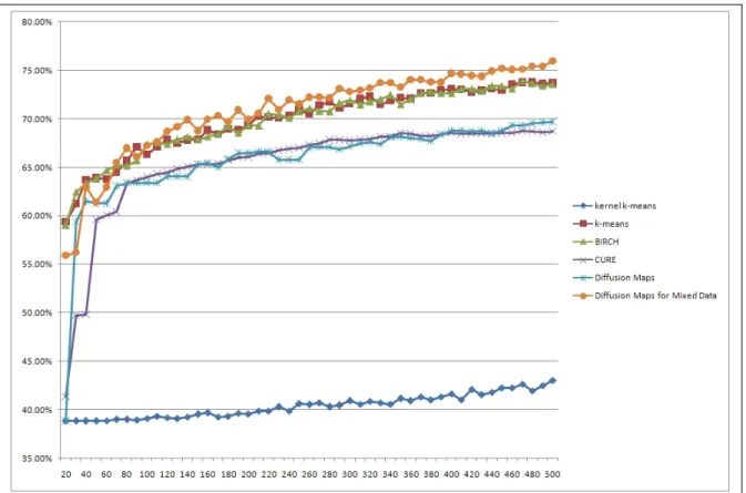
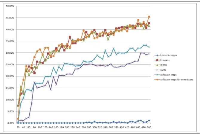
Figure 6.1 shows the clustering accuracy results from each evaluated clustering method.
Figure 6.1: Clustering accuracy results (Eq. 5.2)
For the first 70 clusters,k−means and BIRCH achieve the best results. From the 70th clusters on we can see that our proposed method outperforms all the compared clustering methods.
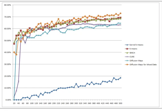
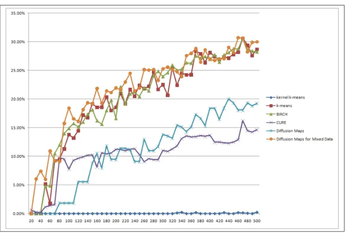
Figure 6.2: Clustering results from 50%-purity (Eq. 5.3)
For the first 100 clusters,k−means and BIRCH achieve the best results. From the 100th clusters on we can see that our proposed method outperforms all the compared clustering methods.
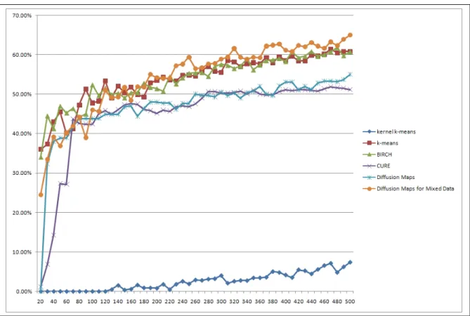
Figure 6.3: Clustering results from 60%-purity (Eq. 5.3)
For the first 170 clusters,k−means and BIRCH achieve the best results. From the 170th clusters on we can see that our proposed method outperforms all the compared clustering methods.
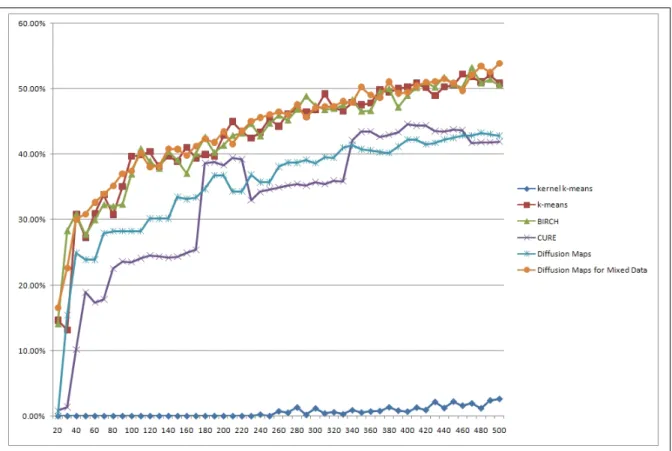
Figure 6.4: Clustering results from 70%-purity (Eq. 5.3)
We can see that our proposed method achieves approximately the same results ask−means and BIRCH.
Figure 6.5: Clustering results from 80%-purity (Eq. 5.3)
We can see that our proposed method achieves approximately the same results ask−means and BIRCH.
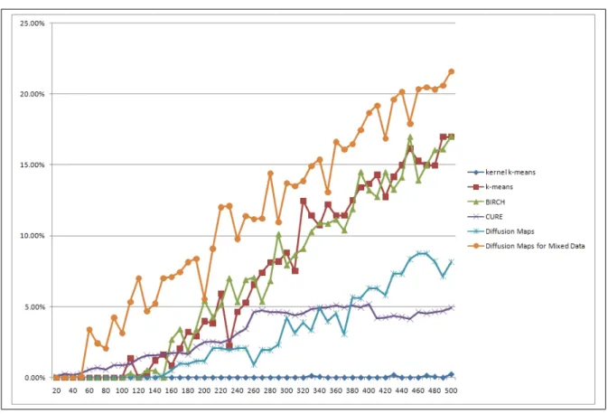
Figure 6.6: Clustering results from 90%-purity (Eq. 5.3)
We can see that our proposed method outperforms all the compared clustering methods. Our method generated more high-purity clusters than any other method.
Figure 6.7: Clustering results from 100%-purity (Eq. 5.3)
We can see that our proposed method outperforms all the compared clustering methods. Our method generated much more absolute-purity clusters than any other method.
7
Conclusions
We presented a new automated technique for clustering mixed data that contains numeric and nominal attributes. The technique is based on automatic transformation of high-dimensional mixed data to common categorical scales. Then, study and analysis of the behavior of the dataset by projecting it onto a low dimensional space is performed. This technique enables to detect normal and abnormal behaviors in the datasets and to discover similarities and dissimilarities among components of these datasets.
An empirical evaluation of our approach was presented. Our method was com-pared to several clustering algorithms. Our experiments showed that our method
outperforms these algorithms in most cases.
References
[1] A. Szlam, M. Maggioni and R. R. Coifman. A general framework for adap-tive regularization based on diffusion processes on graphs. Technical Report YALE/DCS/TR1365, Yale Univ, July 2006.
[2] R. R. Coifman and S. Lafon. Diffusion maps. Applied and Computational Harmonic Analysis, 21(1), 5-30, 2006.
[3] R. R. Coifman and S. Lafon. Geometric harmonics: a novel tool for multiscale out-of-sample extension of empirical functions.Applied and Computational Har-monic Analysis, 21(1), 31-52, 2006.
[4] F. R. K. Chung. Spectral Graph Theory. AMS Regional Conference Series in Mathematics, 92, 1997.
[5] G. Gan, C. Ma, J Wu. Data Clustering: Theory, Algorithms, and Applications. SIAM, 2007.
[6] T. Zhang, R. Ramakrishnan, M Livny. BIRCH: An efficient data clustering method for very large databases. SIGMOD Rec. 25, 2, 103–114., 1996.
[7] M. Ester, H. P. Kriegel, J. Sander, X. Xu. A density-based algorithm for discov-ering clusters in large spatial database with noise. In International Conference on Knowledge Discovery in Databases and Data Mining (KDD-96), Portland, Oregon, pp. 226-231, AAAI Press (1996).
[8] S. Guha, R. Rastogi, K. Shim. CURE: An Efficient Clustering Algorithms for Large Databases. ACM SIGMOD Int. Conf. on Management of Data, Seattle, WA, 1998, pp. 73-84.
[9] L. Kaufman, P. Rousseeuw. Finding groups in Data - An introduction to Cluster Analysis. Wiley. New York: John Wiely & Sons, Inc. 1990.
[10] J. Macqueen. Some methods for classification and analysis of multivariate obser-vations.In Proceedings of the 5th Berkeley symposium on mathematical statistics and probability, volume 1, pages 281-297. Berkeley, CA: University of California Press.
[11] V. Ganti, J. Gehrke, R. Ramakrishnan. CACTUS: Clustering Categorical Data using Summaries. In Proceedings of the 5th ACM SIGKDD International Con-ference on Knowledge Discovery and Data Mining (KDD), San Diego, CA, USA, August 1999, ACM Press, pp. 73–83.
[12] Z. Huang. Extensions to the K-Means Algorithm for Clustering Large Data Sets with Categorical Values. Data Mining and Knowledge Discovery, 2(3), pp. 283–304, 1998.
[13] D. Barbara, J. Couto, Y Li. Coolcat: An Entropy-based algorithm for Categori-cal Clustering. In Proceedings of the 11th ACM Conference on Information and Knowledge Management (CIKM 02), McLean, Virginia, USA, November 2002, ACM Press, pp. 582–589.
[14] S. Guha, R. Rastogi, K. Shim. ROCK: A Robust Clustering Algorithm for Categorical Attributes. Journal of Information Systems, 25(5), pp. 345–366, 2000.
[15] D. Gibson, J. Kleinberg, P. Raghavan. Clustering Categorical Data: An Ap-proach Based on Dynamical Systems. In Proceedings of the 24th International Conference on Very Large Data Bases, (VLDB), New York, NY, USA, August 1998, Morgan Kaufmann, pp. 311–322.
[16] A. Ben-Hur, D. Horn, H. Siegelmann, V. Vapnik. Support vector clustering. J. Mach. Learn. Res., vol. 2, pp. 125–137, 2001.
[17] M. Girolami. Mercer Kernel Based Clustering in Feature Space. IEEE Trans-actions on Neural Networks, 13(4), pp. 780–784, 2002.
[18] R. Zhang, A. Rudnicky. A Large Scale Clustering Scheme for Kernel K-means.In Proceedings of the 16th International Conference on Pattern Recognition (ICPR 02), Quebec City, Canada, August 2002, pp. 289–292.
[19] J. Couto. Kernel K-Means for Categorical Data. Advances in Intelligent Data Analysis VI, Volume 3646, pages 46–56, 2005.
[20] A. Gionis, P. Indyk, R. Motwani. Similarity Search in High Dimensions via Hashing. Proc. of the 25th VLDB Conference, 1999, pp. 518–528.
[21] Cisco Systems, Inc. Cisco SCE 1000 Series Service Control Engine. http://www.cisco.com/en/US/prod/collateral/ps7045/ps6129/ps6133/ps6150/ product data sheet0900aecd801d8564.html.
[22] D. Lazarov, G. David, A. Averbuch. Smart-Sample: An Algorithm for Cluster-ing Large High-Dimensional Datasets. Research report 2008.