ISSN 1841-9836, 10(6):812-824, December, 2015.
Fuzzy Robust Tracking Control for Uncertain Nonlinear
Time-Delay System
Z.-B. Du, T.-C. Lin, T.-B. Zhao
Zhenbin Du Yantai University
Yantai, Shandong, 264005, China [email protected] Tsung-Chih Lin Feng-Chia University Taichung, 40724, Taiwan [email protected] Tiebiao Zhao University of California Merced, CA, 95343, USA [email protected]
Abstract: The problem of fuzzy robust tracking control is investigated for uncer-tain nonlinear time-delay systems. The nonlinear time-delay system is modeled as fuzzy Takagi-Sugeno (T-S) system, and fuzzy logic systems are used to eliminate the uncertainties of the system. A sufficient condition for the existence of fuzzy controller is given in terms of linear matrix inequalities (LMIs) and adaptive law. Based on Lyapunov stability theorem, the fuzzy control scheme guarantees the desired tracking performance in sense that all the closed-loop signals are uniformly ultimately bounded (UUB). Simulation results of 2-link manipulator demonstrate the effectiveness of the developed control scheme.
Keywords: fuzzy T-S model; fuzzy logic systems; nonlinear system; time-delay; tracking control.
1
Introduction
Fuzzy control approach offers a powerful and systematical control methodology to handle nonlinear system. Owing to the superior approximation and reasoning abilities of the fuzzy controller, fuzzy control approach has been applied in different applications. With the extensive efforts of the researchers working on the fuzzy control discipline, fruitful stability analysis results have been obtained to aid the design of stable fuzzy controllers. In [1], a fuzzy T-S model was employed to represent the system dynamics of the nonlinear system. The fuzzy T-S model represents the nonlinear system as a weighted sum of some linear subsystems. This particular structure offers a general framework to represent the nonlinear system which is favorable for system analysis. Fuzzy controllers [2-4] were proposed to handle the nonlinear system represented by the fuzzy T-S model. To avoid the effect of the uncertainties, a matching condition is assumed in [5–7], and an upper bound on uncertainties is introduced in [8–10]. The matching condition and the upper bound in dealing with the uncertainties are effective and feasible. However, there exists certain conservatism. The matching condition is a very conservative assumption and the upper bound may be too big or too small, which adds some difficulties to the controller design. On the other hand, it is well known that fuzzy logic systems can uniformly approximate nonlinear continuous functions to arbitrary accuracy. Thus, fuzzy logic systems are used to model uncertain nonlinear systems in [11–13].
Time delays are frequently encountered in engineering systems. The existence of time delays usually becomes the source of instability and degrading performance of systems. Therefore, stability analysis and controller synthesis for nonlinear time-delay systems are important both in theory and in practice.
By using fuzzy T-S model and fuzzy logic systems, we propose a novel robust tracking con-trol scheme for a class of uncertain nonlinear time-delay system. Fuzzy T-S model is used to approximate the nonlinear system, and a fuzzy state feedback controller is designed to guarantee the stability of the fuzzy system. A compensator based fuzzy logic systems is introduced to eliminate the uncertainties of the system. The fuzzy control scheme ensures the desired tracking performance in sense that all the closed-loop signals are uniformly ultimately bounded (UUB).
The rest of the paper is organized as follows. Section 2 provides the problem formulation. Section 3 develops a procedure of the controller design. Section 4 gives the main result. Section 5 presents simulation examples to illustrate the effectiveness of the proposed method. These are followed by conclusions in Section 6.
2
Problem formulation
Consider the following uncertain nonlinear time-delay system: ˙ x1=x2, · · · ˙ x(β1−1) =xβ1, ˙ xβ1 =f1(x, x(t−τ1),· · · , x(t−τr), u) + ˜f1(x, x(t−τ1),· · ·, x(t−τr), u) +d1, ˙ x(β1+1) =x(β1+2), · · · ˙ xn=fm(x, x(t−τ1),· · · , x(t−τr), u) + ˜fm(x, x(t−τ1),· · ·, x(t−τr), u) +dm, (1) wherex= [x1,· · ·, x(β 1−1) 1 ,· · ·, x(n−βm+1),· · · , x (βm−1) (n−βm+1)] T ∈Rnwithβ 1+β2+· · ·+βm =nand
u∈Rmare the system state and control input, respectively. f
i(i= 1,· · · , m)are known smooth
nonlinear functions, f˜i (i= 1,· · ·, m) are unknown nonlinear uncertainties, τi(i= 1,· · ·, r) are time delays, anddi (i= 1,· · · , m) are external bounded disturbances.
The control objective of this paper is to find a fuzzy tracking controller such that, while maintaining all the closed-loop signals UUB, the system states of nonlinear system (1) follow those of the given stable reference model.
3
Fuzzy model, reference model and fuzzy controller
A fuzzy-model-based control system, formed by a fuzzy model, a reference model, and fuzzy controller connected in a closed-loop, is introduced.
3.1 Fuzzy model
A fuzzy dynamic model has been proposed by Takagi and Sugeno to represent a nonlinear system. The fuzzy dynamic model is described by the following fuzzy IF-THEN rules and will be employed here to deal with the control design problem for the nonlinear system in (1).
Plant Rule i: IFz1(t) is Fi
1 and,· · · ,and zs(t) is Fsi,THEN
˙ x(t) =Aix(t) + r X l=1 Ailx(t−τl) +Biu(t) +d, i= 1,· · ·, L (2)
where z1(t),· · ·, zs(t) are the premise variables, Fji(j = 1,· · · , s) are the fuzzy sets, L is
the number of IF-THEN rules, Ai,Bi and Ail are some constant matrices with compatible
dimensions, Bi=[0,· · · , bTi1,· · ·,0,· · ·, bTim]T ∈ Rn×m with bi1 ∈ Rm,· · · , bim ∈ Rm , and
d= [0,· · · , d1,· · ·,0,· · · , dm]T.
Then, the final output of the fuzzy system is inferred as follows: ˙ x(t) = L X i=1 µi[Aix(t) + r X l=1 Ailx(t−τl)] + L X i=1 µiBiu(t) +d, (3) where µi =vi(z(t)) , L X i=1 vi(z(t)), vi(z(t)) = s Y j=1 Fji(zj(t)) (4)
for all t ≥ 0, and Fji(zj(t)) is the grade of membership of zj(t) in Fji. It can be seen that L
P
i=1
vi(z(t))>0,andvi ≥0(i= 1,· · ·, r) for all t≥0. We have µi≥0(i= 1,· · ·, r), L
P
i=1
µi = 1.
Hence, the nonlinear system (1) can be rearranged as the following equivalent system : ˙ x(t) = L X i=1 µi[Aix(t) + r X l=1 Ailx(t−τl)] + L X i=1 µiBiu(t) +B∆(x, x(t−τ)) +d, (5)
whereB∆(x, x(t−τ)) =B∆(x, x(t−τ1),· · ·, x(t−τr)) denotes the uncertainties between the
non-linear system (1) and the fuzzy model (3), andB =diag[B1,· · ·, Bm]withBi= [0,· · ·,0,1]T ∈
Rβi.
3.2 Reference model
The system states of nonlinear systems (1) are driven to follow those of the following stable reference model
˙
xr(t) =Arxr(t) +r(t), (6)
wherexr(t) is a reference state, r(t) is a bounded reference input, andAr is an asymptotically
stable matrix.
3.3 Fuzzy controller
A fuzzy controller is chosen as
u(t) =ul(t)−uf(t), (7)
where ul(t) denotes the fuzzy state feedback control based on T-S model, and uf(t) is the
adaptive compensator based on fuzzy logic systems. The former is used to stabilize the linear part of system (11), and the latter is used to compensate the uncertainties. ul(t) anduf(t) are
designed as (8) and (10), respectively.
For the fuzzy model represented by (2) or (3), fuzzy state feedback control ul(t) shares the
Control Rule i: IF z1(t) is Fi
1 and,· · ·,and zs(t) is Fsi , THEN
ul(t) =Ki(x(t)−xr(t)), i= 1,· · ·, L.
Hence, the overall state feedback controller ul(t) is given by
ul(t) = L
X
i=1
µiKi(x(t)−xr(t)), (8)
whereKi(i= 1,2,· · · , L)are matrices with proper dimensions and satisfy the following
inequal-ities ¯ ATijP +PA¯ij + r X l=1 α−1l PA¯ilA¯TilP + r X l=1 αlI+ 1 ρ2P P + ¯Q <0, i, j= 1,· · ·, L, (9) whereA¯ij = " Ai+BiKj −BiKj 0 Ar # ,A¯il= " Ail 0 0 0 #
,Q¯=diag{2Q,2Q},P andQ are some symmetric and positive definite matrices, andαl(l= 1,· · ·, r)are positive constants.
The adaptive compensator based on fuzzy logic systems uf(t)are as follows:
uf(t) = ( E−1uˆ(x, x(t−τ)|Θ), if E is nonsigular ET(I+EET)−1uˆ(x, x(t−τ)|Θ), if E is sigular (10) whereEi = [bTi1,· · ·, bTim]T ∈Rm×m,E = L P i=1
µiEi, and uˆ(x, x(t−τ)|Θ) is constructed by fuzzy
logic systems. The weightΘ is an adaptive parameter, which is adapted by ˙
Θ =η1ΨT(x, x(t−τ)) ¯BTPx,˜ (11)
whereη1is a positive constant,Ψ(x, x(t−τ))is a fuzzy basis-function matrix, andx˜= [xT, xTr]T.
In the following, we explain the solution of the inequalities (9) and the construction of fuzzy logic systemsuˆ(x, u|Θ).
1) By Schur complements, the inequalities (9) are transformed into the LMIs. For the conve-nience of design,Pis chosen as the formP =diag{P1, P2}, whereP1, P2 are some symmetric and positive definite matrices. The inequalities (9) are equivalent to the following matrix inequalities
S11 −P1BiKj 0 −(BiKj)TP1 S22 P2 0 P2 −ρ2I <0, i, j= 1,2,· · ·, L, (12) WhereS11=P1(Ai+BiKj) + (Ai+BiKj)TP1+ r P l=1 α−1l P1AilATilP1+ r P l=1 αlI+ρ12P1P1+ 2Q, S22=P2Ar+ATrP2+ r X l=1 αlI + 2Q.
The matrix inequalities (12) imply S11 < 0. Let W = P1−1 and Yj = KjW. S11 < 0 is
equivalent to the LMIs with prescribedQand αl(l= 1,· · · , r),
S W W −( r P l=1 αlI + 2Q)−1 <0, i, j= 1,2,· · ·, L (13)
whereS=AiW +W ATi +BiYj+ (BiYj)T + r
P
l=1
α−1l AilATil + (ρ2)−1I.
By solving the LMIs (13), P1 and Kj(j = 1,2,· · ·, L) could be obtained. And then, by
substituting P1 and Kj(j = 1,2,· · · , L) into (12), (12) becomes standard LMIs. We can easily
solve P2 from (12). Therefore, the common solution P andKj(j= 1,2,· · ·, L)could be found.
Remark 1: Either the matching condition or the upper bound is related to a large number
of matrix operations. Without the matching condition and the upper bound, the dimension of the LMIs of this paper is reduced.
2) Fuzzy adaptive systems consist of four main components: fuzzy rule base, fuzzy inference engine, fuzzifier and defuzzifier [11]. The fuzzy rule base is composed of a collection of IF-THEN inference rules:
Rl: IFx1 isAl1,· · · , xn isAlnŁŹTHEN y isGl(l= 1,· · ·p)
whereAl
i(i= 1,· · · , l)and Gl(l= 1,· · ·p)are fuzzy sets. Thekth element of∆(x, x(t−τ))is of
the following form:
ˆ ∆k(x, x(t−τ)|θk) =ξTk(x, x(t−τ))θk, whereθk= (θk1,· · · , θ p k)T ∈Rp, ξkT(x, x(t−τ)) = (ξk1,· · · , ξ p k)∈Rp, ξkl = n Y i=1 µFl i(xi, xi(t−τ)) , p X l=1 n Y i=1 µFl i(xi, xi(t−τ)), µF l i(xi, xi(t−τ)) =µF l i(xi) r Y j=1 µFl i(xi(t−τj)), and µFl
i(xi)(i= 1,2,· · · , n) are the membership functions.
In this paper, fuzzy logic systems are constructed to eliminate the uncertainties∆(x, x(t−τ)).
The approximation form is given as follows: ˆ
∆(x, x(t−τ)|Θ) = Ψ(x, x(t−τ))Θ, (14) whereΨ(x, x(t−τ)) =diag[ξT
1(x, x(t−τ)),· · ·, ξmT(x, x(t−τ))],Θ = [θT1, θ2T,· · ·, θmT]T.
Define the optimal the parameter Θ∗ as Θ∗= arg min
Θ∈Ω1
[ sup
x∈U1
|ˆu(x, x(t−τ)|Θ)−∆(x, x(t−τ))|], (15)
whereU1={x∈Rn:kxk ≤N},Ω1={Θ∈Rpm:kΘk ≤M}. U1,Ω1 denote the sets of suitable
bounds onx,Θrespectively, N, Mare upper bounds.
The approximation error for the function∆(x, x(t−τ))can be expressed as ˆ
∆(x, x(t−τ)|Θ)−∆(x, x(t−τ)) = Ψ(x, x(t−τ)) ˜Θ +w, (16) whereΘ = Θ˜ −Θ∗ the estimation error for Θ,w= [w
1,· · ·, wm]Tis a residual term.
Remark 2: In order to guarantee kΘk ≤ M, the adaptive law (11) must be modified by the
projection algorithm [11] as follows:
˙ Θ =
(
η1ΨT(x, x(t−τ)) ¯BTPx,˜ if(kΘk<M)or(kΘk=M andx˜TPB¯ Ψ(x, x(t−τ))Θ≤0)
PΘ[.],ifkΘk=M and x˜TPB¯ Ψ(x, x(t−τ))Θ>0
where PΘ[.]=η1ΨT(x, x(t−τ)) ¯BTPx˜−η1 ˜x
TP¯
BΨ(x,x(t−τ))Θ
4
Stability analysis
Substituting (11) into (11) yields˙ x(t) = L X i=1 µi[Aix(t) + r X l=1 Ailx(t−τl)] + L X i=1 L X j=1 µiµjBiKj(x(t)−xr(t)) −B(ˆu(x, x(t−τ)|Θ)−∆(x, x(t−τ))) +d. (17) Letx˜(t) = [xT(t), xrT(t)]T, andB¯ = [ BT 0 ]T. By using (11) and (17), a new extended
closed-loop system is as follows:
˙˜ x(t) = L X i=1 L X j=1 µiµj[ ¯Aijx˜(t) + r X l=1 ¯ Ailx˜(t−τl)] + ¯B(−(ˆu(x, x(t−τ)|Θ)−∆(x, x(t−τ))) +d′, (18)
whered′= [dT, rT(t)]T. When fuzzy logic systemsuˆ(x, x(t−τ)|Θ)could eliminate∆(x, x(t−τ)),
the closed-loop system (18) is stable.
By denoting w′ = [ ¯wT, rT(t)]T,w¯ = [0,· · ·, d
1−w1,· · · ,0,· · · , dm−wm]T and using (14),
the closed-loop system (18) could be rewritten as
˙˜ x(t) = L X i=1 L X j=1 µiµj[ ¯Aijx˜(t) + r X l=1 ¯ Ailx˜(t−τl)] + ¯B(−Ψ(x, x(t−τ)) ˜Θ) +w′. (19)
From the above analysis, we have the following conclusion.
Theorem 1. Given a matrixQ > 0, scalarsρ > 0,αl(l = 1,· · · , r) > 0, η1 > 0.If there exist
matricesP > 0,Kj(j = 1,2,· · ·, L) such that the inequalities (9) hold. If the updating law for
fuzzy logic systems is chosen as (11). Then there exists a controller (11) with the fuzzy state feedback controller (8) and the adaptive compensator (10) such that, while maintaining all the closed-loop signals UUB, the following tracking performance(20) is achieved
Z T 0 (x(t)−xr(t))TQ(x(t)−xr(t))dt≤x˜T(0)Px˜(0) + 1 η1 ˜ ΘT(0) ˜Θ(0) +ρ2 Z T 0 (w′Tw′)dt. (20)
Proof: Consider the following Lyapunov-Krasoviskii candidate
V = 1 2x˜ TPx˜+1 2 r X l=1 Z t t−τl αlx˜T(v)˜x(v)dv+ 1 2η1 ˜ ΘTΘ˜, (21)
whereV˙ = ˙V1+ ˙V2,V˙1andV˙2 are given in (22) and (26), respectively.
˙ V1= 1 2( L X i=1 L X j=1 µiµj[ ¯Aijx˜(t) + r X l=1 ¯ Ailx˜(t−τl)])TPx˜(t) + 1 2x˜ T(t)P( L X i=1 L X j=1 µiµj[ ¯Aijx˜(t) + r X l=1 ¯ Ailx˜(t−τl)]) + 1 2w′ TP x(t) +1 2x T(t)P w′+1 2 r X l=1 αlx˜T(t)˜x(t)− 1 2 r X l=1 αlx˜T(t−τl)˜x(t−τl) ≤ 1 2( L X i=1 L X j=1 µiµj[˜xT(t) ¯ATijPx˜(t)+˜xT(t)PA¯ijx˜(t)+ r X l=1 α−1l x˜T(t)PA¯ilA¯TilPx˜(t)+ r X l=1 αlx˜T(t−τl)˜x(t−τl)]
−1 2( 1 ρP x(t)−ρw′) T(1 ρP x(t)−ρw′) + 1 2ρ 2w′Tw′+ 1 2ρ2x˜ T(t)P Px˜(t) +1 2 r X l=1 αlx˜T(t)˜x(t) −12 r P l=1 αlx˜T(t−τl)˜x(t−τl) ≤ 1 2 L X i=1 L X j=1 µiµjx˜T(t)( ¯ATijP+PA¯ij+ r X l=1 α−1l PA¯ilA¯TilP+ r X l=1 αlI+ 1 ρ2P P)˜x(t)+ 1 2ρ 2w′Tw′. (22)
Substituting (9) into (22) yields ˙ V1 ≤ −1 2x˜ T(t) ¯Qx˜(t) +1 2ρ 2w′Tw′. (23) By using (11), V2 = [˜xTPB¯(−(Ψ(x, x(t−τ)) ˜Θ) + 1 η1Θ˜ TΘ] = 0˙ . (24) From (23)-(24), ˙ V ≤ −1 2x˜ T(t) ¯Qx˜(t) +1 2ρ 2w′Tw′. (25) Whenk˜x(t)k > λ ρ min( ¯Q)kw′k, ˙
V <0.Thus, the closed-loop system consisting of (1), (11), (8) and
(10) is UUB . ✷ Note that Z T 0 (x(t)−xr(t))TQ(x(t)−xr(t))dt ≤ Z T 0 ˜ xT(t) ¯Qx˜(t)dt.
Integrating the above equation (25) fromt= 0 toTyields (20).
5
Simulation example
In this section, we provide an example to verify the effectiveness of the proposed control scheme.
Example: Consider the following 2-link manipulator system in [14]
¨ q(t) +C(q,q˙) ˙q(t) +g(q) =B(q)u(t) + r X i=1 ξi(t)q(t−τi) +d′, (26) whereC(q,q˙) =H−1(q)C′(q,q˙), g(q) =H−1(q)g′(q), B(q) =H−1(q),d′=H−1(q)d,q = [q1, q2]T,
ξi(t)(i= 1,· · · , r)are uncertain and bounded, and dis the external bounded disturbance.
The reference model is as follows: ˙ xr(t) =Arxr(t) +r(t), (27) whereAr =diag{Ar1, Ar2},Ar1 =Ar2 = " 0 1 −6 −5 # , r(t) = [0, r1(t),0, r2(t)]T,r1(t) =r2(t) = 3 sin(2t).
Step1: Denotex1 =q1, x2 = ˙q1, x3 =q2,andx4= ˙q2. Then, (26) can be written as a fourth-dimension system. A nine-rule fuzzy T-S model is used to approximate the nonlinear 2-link manipulator system atx1 =−π2,0,π2 andx3=−π2,0,π2, where
A1 = 0 1 0 0 5.927 −0.001 −0.315 −0.0000084 0 0 0 1 −6.859 0.002 3.155 0.0000062 , A2= 0 1 0 0 3.0428 −0.0011 −0.1791 −0.0002 0 0 0 1 −3.5436 0.0313 2.5611 0.0000114 , A3 = 0 1 0 0 6.2728 0.003 0.4339 −0.0001 0 0 0 1 −9.1041 0.0158 −1.0574 −0.000032 , A4 = 0 1 0 0 6.4535 0.0017 1.2427 −0.0002 0 0 0 1 −3.1873 0.0306 −5.1911 −0.000018 , A5 = 0 1 0 0 11.1336 0 −1.8145 0 0 0 0 1 −9.0918 0 9.1638 0 , A6= 0 1 0 0 6.1702 −0.001 1.687 −0.0002 0 0 0 1 −2.3559 0.0314 4.5298 −0.000011 , A7 = 0 1 0 0 6.1206 0.0041 0.6205 0.0001 0 0 0 1 8.8794 0.0193 −1.0119 0.000044 , A8 = 0 1 0 0 3.6421 −0.0018 0.0721 0.0002 0 0 0 1 2.429 −0.0305 2.9832 −0.000019 , A9= 0 1 0 0 6.2933 −0.0009 0.2188 −0.000012 0 0 0 1 −7.4649 0.0024 3.2693 −0.0000092 , A11=A21=A31=A41=A51=A61=A71=A81=A91= 0 0 0 0 0.01 0 0 0 0 0 0 0 0 0 0 0 , A12=A22=A32=A42=A52=A62=A72=A82=A92= 0 0 0 0 0 0 0 0 0 0 0 0 0 0 0.01 0 , B1 = " 0 1 0 −1 0 −1 0 2 #T , B2= " 0 0.5 0 0 0 0 0 1 #T , B3 = " 0 1 0 1 0 1 0 2 #T , B4 = " 0 0.5 0 0 0 0 0 1 #T , B5= " 0 1 0 −1 0 −1 0 2 #T , B6= " 0 0.5 0 0 0 0 0 1 #T ,
B7= " 0 1 0 1 0 1 0 2 #T , B8 = " 0 0.5 0 0 0 0 0 1 #T , B9= " 0 1 0 −1 0 −1 0 2 #T .
The membership functions are adopted as the triangle type.
Step 2: On the basis of Theorem1, withα1 = 0.005,α2= 0.005, andρ= 1,we have
K1 = " -76.9685 -42.9566 -19.6919 -8.9116 6.0025 -0.4619 -51.4252 -25.0336 # , K2 = " -77.7828 -42.8754 -13.6211 -5.9413 8.7179 1.2251 -50.6614 -24.6859 # , K3= " -76.8347 -42.9089 -19.8204 -8.9785 5.8595 -0.5257 -51.3739 -25.0109 # , K4 = " -77.7828 -42.8754 -13.6211 -5.9413 8.7179 1.2251 -50.6614 -24.6859 # , K5 = " -77.7828 -42.8754 -13.6211 -5.9413 8.7179 1.2251 -50.6614 -24.6859 # , K6 = " -77.7828 -42.8754 -13.6211 -5.9413 8.7179 1.2251 -50.6614 -24.6859 # , K7 = " -79.8424 -43.4072 -6.0780 -2.2626 12.7745 3.6898 -50.2150 -24.4989 # , K8 = " -77.7828 -42.8754 -13.6211 -5.9413 8.7179 1.2251 -50.6614 -24.6859 # , K9= " -80.1162 -43.5088 -5.8152 -2.1328 13.0509 3.8147 -50.3242 -24.5472 # .
Step 3: In fuzzy adaptive compensator, the membership functions are selected as
µF1 i(xi) = 1 1 + exp[5(xi+ 0.8)] , µF2 i(xi) = exp[−(xi+ 0.6) 2], µ F3 i(xi) = exp[−(xi+ 0.4) 2], µF4 i(xi) = exp[−(xi) 2], µ F5 i(xi) = exp[−(xi−0.4) 2], µ F6 i(xi) = exp[−(xi−0.6) 2], µF7 i(xi) = 1 1 + exp[5(xi−0.8)] , i= 1,2,· · · ,4.
Step 4: Some parameters are choose as
η1 = 10, r= 2, τ1 = 0.5, τ2= 1, ξ1(t) =5+20sin(5t),andξ1(t) =1+15cos(5t), Θ(0) = [0.2,0.2,0.2,0.2,0.2,0.2,0.2,0.2,0.2,0.2,0.2,0.2,0.2,0.2,0.2],
(x1(0), x2(0), x3(0), x4(0), xr1(0), xr2(0), xr3(0), xr4(0)) = (0.4,0,−0.4,0,0,0,0,0).
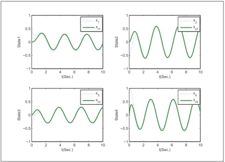
By using the method in Theorem 1, the tracking performances ofx1(t), x2(t), x3(t), x4(t)are shown in Fig.1,and the control effortsu1(t) andu2(t) are given in Fig.2,respectively.
0 2 4 6 8 10 −1 −0.5 0 0.5 1 t(Sec.) State1 0 2 4 6 8 10 −1 −0.5 0 0.5 1 t(Sec.) State2 0 2 4 6 8 10 −1 −0.5 0 0.5 1 t(Sec.) State3 0 2 4 6 8 10 −1 −0.5 0 0.5 1 t(Sec.) State4 x 1 x r1 x 2 x r2 x 3 x r3 x 4 x r4
Figure 1: The responses ofx1,x2,x3,x4,xr1,xr2,xr3andxr4
0 2 4 6 8 10 −80 −60 −40 −20 0 20 40 t(Sec.) Control1 0 2 4 6 8 10 −10 0 10 20 30 40 50 60 70 Control2 t(Sec.)
Figure 2: The control inputsu1,u2
0 2 4 6 8 10 −1 −0.5 0 0.5 1 t(Sec.) State1 0 2 4 6 8 10 −1 −0.5 0 0.5 1 t(Sec.) State2 0 2 4 6 8 10 −1 −0.5 0 0.5 1 t(Sec.) State3 0 2 4 6 8 10 −1 −0.5 0 0.5 1 t(Sec.) State4 x 1 x r1 x 2 x r2 x 3 xr3 x 4 xr4
0 2 4 6 8 10 −1 −0.5 0 0.5 1 t(Sec.) Sate1 0 2 4 6 8 10 −1 −0.5 0 0.5 1 t(Sec.) Sate2 0 2 4 6 8 10 −1 −0.5 0 0.5 1 t(Sec.) Sate3 0 2 4 6 8 10 −1 −0.5 0 0.5 1 t(Sec.) Sate4 x1 xr1 x2 xr2 x3 xr3 x4 xr4
Figure 4: The responses ofx1,x2,x3,x4,xr1,xr2,xr3andxr4
0 2 4 6 8 10 −0.1 0 0.1 0.2 0.3 0.4 t(Sec.) State1 0 2 4 6 8 10 −0.8 −0.6 −0.4 −0.2 0 0.2 State2 t(Sec.) 0 2 4 6 8 10 −0.4 −0.3 −0.2 −0.1 0 0.1 t(Sec.) State3 0 2 4 6 8 10 −0.5 0 0.5 1 t(Sec.) State4 x4 x r4 x2 xr2 x 1 xr1 x 3 xr3
Figure 5: The responses ofx1,x2,x3,x4,xr1,xr2,xr3andxr4
0 2 4 6 8 10 −15 −10 −5 0 5 t(Sec.) Control1 0 2 4 6 8 10 −5 0 5 10 15 t(Sec.) Control2 u1 u2
Whenτ1 = 1,τ2 = 1, simulation results are shown in Fig.3.Whenτ1 = 1,τ2 = 2, simulation results are shown in Fig.4.
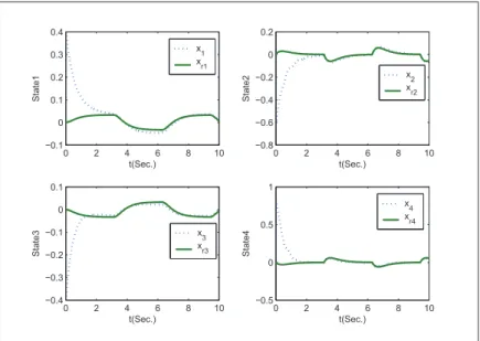
When r1(t)andr2(t) are square waves having an amplitude ±0.2 with a period of 2π, the
tracking performances of x1(t), x2(t), x3(t), x4(t) are shown in Fig. 5, and the control efforts
u1(t)and u2(t) are given in Fig.6.
Simulation results illustrate that the proposed controller design is effective and feasible.
6
Conclusion
Based on fuzzy technique, a novel tracking control scheme is presented for uncertain non-linear time-delay system. As main contribution of this paper, we design a novel fuzzy tracking controller, which is independent of the matching condition or the upper bound for the uncer-tainties. Furthermore, the tracking control design for discrete nonlinear systems is also developed.
Acknowledgment
This work was supported by the National Natural Science Foundation of China(61203320,61273128), Shandong Natural Science Foundation(ZR2014FL023) and the project of Shandong Province higher educational science and technology program(J14LN70).
Bibliography
[1] T. Takagi; M. Sugeno. (1985); Fuzzy identification of systems and its applications to mod-eling and control, IEEE Transactions on Systems, Man, and Cybernetics, ISSN 0018-9472, SMC-15(1):116-132.
[2] J.-W. Wang; H.-N. Wu; H.-X. Li. (2011); Distributed fuzzy control design of nonlinear hyper-bolic PDE systems with application to nonisothermal plug-flow reactor, IEEE Transactions on Fuzzy Systems, ISSN 1063-6706, 19(3): 514 - 526.
[3] D.W. Kim;H.J. Lee. (2012); Sampled-data observer-based output-feedback fuzzy stabiliza-tion of nonlinear systems: Exact discrete-time design approach, Fuzzy Sets and Systems, ISSN 0165-0114, 201(16): 20-39.
[4] G.K. Koo;J.B. Park;Y.H. Joo. (2013); Guaranteed cost sampled-data fuzzy control for non-linear systems: a continuous-time Lyapunov approach, IET Control Theory and Applica-tions, ISSN 1751-8644, 7(13): 1745–1752.
[5] Y.-S. Zhang;S.-Y. Xu;Y. Zou;J.-J. Lu. (2011); Delay-dependent robust stabilization for un-certain discrete-time fuzzy Markovian jump systems with mode-dependent time delays, Fuzzy Sets and Systems, ISSN 0165-0114, 164(1):66-81.
[6] J. Yoneyama. (2012); Robust sampled-data stabilization of uncertain fuzzy systems via input delay approach, Information Sciences, ISSN 0020-0255, 198 (1): 169-176.
[7] J. Yoneyama. (2013); Robust H8 filtering for sampled-data fuzzy systems, Fuzzy Sets and Systems, ISSN 0165-0114, 217(16) : 110-129.
[8] Z.-Y. Xi;G. Feng;T. Hesketh. (2011); Piecewise Integral Sliding-Mode Control for T–S Fuzzy Systems, IEEE Transactions on Fuzzy Systems, ISSN 1063-6706, 19(1): 65-74.
[9] J. Chen;F.Sun;Y.Yin;C.Hu. (2011); State feedback robust stabilization for discrete-time fuzzy singularly perturbed systems with parameter uncertainty, IET Control Theory and Applications, ISSN 1751-8644, 5(10): 1195 - 1202.
[10] C.-H. Lien;J.-D. Chen;K.-W. Yu;L.-Y.Chung. (2012); Robust delay-dependent H8 control for uncertain switched time-delay systems via sampled-data state feedback input, Computers and Mathematics with Applications, ISSN 0898-1221 , 64(5):1187-1196.
[11] L.-X. Wang. (1993); Stable adaptive fuzzy control of nonlinear systems, IEEE Transactions on Fuzzy Systems, ISSN 1063-6706,1(3):146-155.
[12] W.-S. Chen;Z.-Q. Zhang. (2010); Globally stable adaptive backstepping fuzzy control for output-feedback systems with unknown high-frequency gain sign, Fuzzy Sets and Systems, ISSN 0165-0114,161(6): 821-836.
[13] Z.-B. Du;T.-C. Lin;V. E. Balas. (2012); A new approach to nonlinear tracking control based on fuzzy approximation, International Journal of Computers, Communications and Control, ISSN 1841-9836,7(1):61-72.
[14] W.-S. Yu. (2004); Tracking-based adaptive fuzzy-neural control for MIMO uncertain robotic systems with time delays, Fuzzy Sets and Systems, ISSN 0165-0114,146(3): 375-401.