Diverse near neighbor problem

(1)

Diverse Near Neighbor Problem

[Extended Abstract]

Sofiane Abbar

QCRI, Doha, Qatar

Sihem Amer-Yahia

CNRS, LIG, Paris, France

Piotr Indyk

MIT, Cambridge, MA, USA

Sepideh Mahabadi

MIT, Cambridge, MA, USA

Kasturi R. Varadarajan

U Iowa, Iowa City, IA, USA

ABSTRACT

Motivated by the recent research on diversity-aware search, we investigate the k-diverse near neighbor reporting prob-lem. The problem is defined as follows: given a query point

q, report themaximum diversitysetSofkpoints in the ball of radiusr around q. The diversity of a set S is measured by the minimum distance between any pair of points inS

(the higher, the better).

We present two approximation algorithms for the case where the points live in a d-dimensional Hamming space. Our algorithms guarantee query times that are sub-linear inn and only polynomial in the diversity parameter k, as well as the dimensiond. For low values ofk, our algorithms achieve sub-linear query times even if the number of points within distancerfrom a queryqis linear inn. To the best of our knowledge, these are the first known algorithms of this type that offer provable guarantees.

Categories and Subject Descriptors

F.2.2 [Nonnumerical Algorithms and Problems]: Ge-ometrical problems and computations; E.2 [Data Storage Representations]: Hash-table representations

Keywords

Near Neighbor, Diversity, Core-set, Sub-linear

1. INTRODUCTION

The near neighbor reporting problem (a.k.a. range query) is defined as follows: given a collectionP ofnpoints, build a data structure which, given any query point, reports all data points that are within a given distancerto the query. The problem is of major importance in several areas, such as databases and data mining, information retrieval, image and video databases, pattern recognition, statistics and data analysis. In those application, the features of each object of

Permission to make digital or hard copies of all or part of this work for personal or classroom use is granted without fee provided that copies are not made or distributed for profit or commercial advantage and that copies bear this notice and the full citation on the first page. To copy otherwise, to republish, to post on servers or to redistribute to lists, requires prior specific permission and/or a fee.

interest (document, image, etc) are typically represented as a point in ad-dimensional space and the distance metric is used to measure similarity of objects. The basic problem then is to perform indexing or similarity searching for query objects. The number of features (i.e., the dimensionality) ranges anywhere from tens to thousands.

One of the major issues in similarity search is how many answers to retrieve and report. If the size of the answer set is too small (e.g., it includes only the few points closest to the query), the answers might be too homogeneous and not informative [6]. If the number of reported points is too large, the time needed to retrieve them is high. Moreover, long answers are typically not very informative either. Over the last few years, this concern has motivated a significant amount of research on diversity-aware search [8, 18, 5, 12, 17, 16, 7] (see [6] for an overview). The goal of that work is to design efficient algorithms for retrieving answers that are bothrelevant(e.g., close to the query point) anddiverse. The latter notion can be defined in several ways. One of the popular approaches is to cluster the answers and return only the cluster centers [6, 8, 14, 1]. This approach however can result in high running times if the number of relevant points is large.

Our results.

In this paper we present two efficient approximate algo-rithms for thek-diverse near neighborproblem. The prob-lem is defined as follows: given a query point, report the

maximum diversity set S of k points in the ball of radius

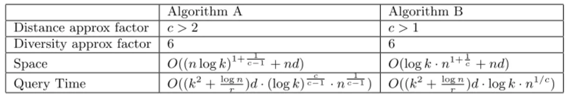
r around q. The diversity of a set S is measured by the minimum distance between any pair of points inS. In other words, the algorithm reports the approximate solution to the k-center clustering algorithm applied to the list points that are close to the query. The running times, approxi-mation factors and the space bounds of our algorithms are given in Table 1. Note that the Algorithm A is dominated by Algorithm B; however, it is simpler and easier to analyze and implement, and has been used in applications before for diverse news retrieval [1].

The key feature of our algorithms is that they guarantee query times that are sub-linear innand polynomial in the diversity parameterkand the dimensiond, while at the same time providing constant factor approximation guarantees1 for the diversity objective. Note that for low values ofkour 1_{Note that approximating the diversity objective is} in-evitable, since it is NP-hard to find a subset of sizekwhich

(2)

Algorithm A Algorithm B Distance approx factor c >2 c >1

Diversity approx factor 6 6

Space O((nlogk)1+c−11 ₊_nd₎ _O_(log_k_·_n1+1c+nd)

Query Time O((k2+log_rn)d·(logk)c−c1 _·_nc−11₎ _O₍₍_k2₊logn

r )d·logk·n

1/c

)

Table 1: Performance of our algorithms

algorithms have sub-linear query timeseven ifthe number of points within distancerfromqis linear inn. To the best of our knowledge, these are the first known algorithms of this type with provable guarantees. One of the algorithms (Algorithm A) is closely related to algorithms investigated in applied works [1, 14]. However, those papers did not provide rigorous guarantees on the answer quality.

1.1 Past work

In this section we present an overview of past work on (approximate) near neighbor and diversity aware search that are related to the results in this paper.

Near neighbor.

The near neighbor problem has been a subject of exten-sive research. There are several efficient algorithms known for the case when the dimensiondis “low”. However, despite decades of intensive effort, the current solutions suffer from either space or query time that is exponential ind. Thus, in recent years, several researchers proposed methods for overcoming the running time bottleneck by using approxi-mation. In the approximate near neighbor reporting/range query, the algorithm must outputallpoints within the dis-tancer fromq, and can also outputsomepoints within the distancecr fromq.

One of the popular approaches to near neighbor prob-lems in high dimensions is based on the concept of locality-sensitive hashing(LSH) [10]. The idea is to hash the points using several (sayL) hash functions so as to ensure that, for each function, the probability of collision is much higher for objects which are close to each other than for those which are far apart. Then, one can solve (approximate) near neigh-bor reporting by hashing the query point and retrieving all elements stored in buckets containing that point. This ap-proach has been used e.g., for the E2LSH package for high-dimensional similarity search [4].

The LSH algorithm has several variants, depending on the underlying distance functions. In the simplest case when the dis-similarity between the query points is defined by the Hamming distance, the algorithm guarantees that (i) each point within the distancerfrom from q is reported with a constant (tunable) probability and (ii) the query time is at mostO(d(n1/c₊_|_P

cr(q)|)), wherePR(q) denotes the set of

points inP with the distanceRfromq. Thus, if the size of the answer setPcr(q) is large, the efficiency of the algorithm

decreases. Heuristically, a speedup can be achieved [14] by clustering the points in each bucket and retaining only the cluster centers. However, the resulting algorithm did not have any guarantees (until now).

maximizes the diversity with approximation factor a < 2 [13].

Diversity.

In this paper we adopt the ”content-based” definition of di-versity used e.g., in [6, 8, 14, 1, 7]. The approach is to report

k answers that are ”sufficiently different” from each other. This is formalized as maximizing the minimum distance be-tween any pair of answers, the average distance bebe-tween the answers, etc. In this paper we use the minimum distance for-mulation, and use the greedy clustering algorithm of [9, 13] to find thek approximately most diverse points in a given set.

To the best of our knowledge, the only prior work that ex-plicitly addresses our definition of thek-diverse near neigh-bor problem is [1]. It presents an algorithm (analogous to Algorithm A in this paper, albeit for the Jaccard coefficient as opposed to the Hamming metric) and applies it to prob-lems in news retrieval. However, that paper does not pro-vide any formal guarantees on the accuracy of the reported answers.

1.2 Our techniques

Both of our algorithms use LSH as the basis. The key chal-lenge, however, is in reducing the dependence of the query time on the size of the setPcr(q) of points close to q. The

first algorithm (Algorithm A) achieves this by storing only thekmost diverse points per each bucket. This ensures that the total number of points examined during the query time is at mostO(kL), whereLis the number of hash functions. However, proving the approximation guarantees for this al-gorithm requires that no outlier (i.e., point with distance

> cr fromq) is stored in any bucket. Otherwise that point could have been selected as one of thek diverse points for that bucket, replacing a “legitimate” point. This require-ment implies that the algorithm works only if the distance approximation factorcis greater than 2.

The 6-approximation guarantee for diversity is shown by using the notion of coresets [2]. It is easy to see that the maximum k-diversity of a point set is within a factor of 2 from the optimal cost of its (k−1)-center clustering cost. For the latter problem it is known how to construct a small subset of the input point set (acoreset) such that for any set of cluster centers, the costs of clustering the coreset is within a constant factor away from the cost of clustering the whole data set. Our algorithm then simply computes and stores only a coreset for each LSH bucket. Standard coreset properties imply that the union of coresets for the buckets touched by the query point q is a coreset for all points in those buckets. Thus, the union of all coresets provides a sufficient information to recover an approximately optimal solution to all points close toq.

In order to obtain an algorithm that works for arbitrary

c >1, we need the algorithms to be robust to outliers. The standard LSH analysis guarantees that that the number of outliers in all buckets is at mostO(L). Algorithm B achieves the robustness by storing arobustcoreset [11, 3], which can

(3)

tolerate some number of outliers. Since we do not know a priori how many outliers are present in any given bucket, our algorithm stores a sequence of points that represents a coreset robust to an increasing number of outliers. During the query time the algorithm scans the list until enough points have been read to ensure the robustness.

2. PROBLEM DEFINITION

Let (∆, dist) be a d-dimensional metric space. We start from two definitions.

Definition 1. For a given setS ∈∆, itsdiversityis de-fined as the minimum pairwise distance between the points of the set, i.e.,div(S) = minp,p0∈Sdist(p, p

0

)

Definition 2. For a given set S ∈ ∆, its k-diversity is defined as the maximum achievable diversity by choosing a subset of sizek, i.e.,divk(S) = maxS0_⊂_S,_|_S0_|₌_kdiv(S0). We

also call the maximizing subsetS0 the optimal k-subset

ofS. Note thatk-diversity is not defined in the case where

|S|< k.

To avoid dealing with k-diversity of sets of cardinality smaller than k, in the following we adopt the convention that all pointsp in the input point setP are duplicatedk

times. This ensures that for all non-empty sets S consid-ered in the rest of this paper the quantitydivk(S) is well

defined, and equal to 0 if the number of distinct points in

S is less than k. It can be easily seen that this leaves the space bounds of our algorithms unchanged.

Thek-diverse Near Neighbor Problemis defined as follows: given a query pointq, report a setS such that: (i)

S ⊂P ∩B(q, r), whereB(q, r) ={p|dist(p, q) ≤r}is the ball of radiusr, centered at q; (ii)|S| =k; (iii) div(S) is maximized.

Since our algorithms are approximate, we need to define theApproximate k-diverse Near Neighbor Problem. In this case, we require that for some approximation factors

c > 1 andα > 1: (i) S ⊂P ∩B(q, cr); (ii)|S| =k; (iii)

div(S)≥ 1

αdivk(P∩B(q, r)).

3. PRELIMINARIES

3.1 GMM Algorithm

Suppose that we have a set of pointsS⊂∆, and want to compute an optimalk-subset ofS. That is, to find a subset ofkpoints, whose pairwise distance is maximized. Although this problem is NP-hard, there is a simple 2-approximate greedy algorithm [9, 13], calledGM M.

In this paper we use the following slight variation of the GMM algorithm2_{. The algorithm is given a set of points}

S, and the parameterk as the input. Initially, it chooses some arbitrary point a ∈ S. Then it repeatedly adds the next point to the output set until there arek points. More precisely, in each step, it greedily adds the point whose min-imum distance to the currently chosen points is maximized. Note that the convention that all points havek duplicates implies that if the input point setS contains less thank dis-tinct points, then the outputS0contains all of those points. 2_{The proof of the approximation factor this variation} achieves is virtually the same as the proof in [13]

Algorithm 1GMM

InputS: a set of points,k: size of the subset

OutputS0: a subset ofS of sizek.

1: S0← An arbitrary point a

2: fori= 2→kdo

3: findp∈S\S0 which maximizes minx∈S0dist(p, x)

4: S0←S0∪ {p}

5: end for

6: return S0

Lemma 1. The running time of the algorithm isO(k·|S|), and it achieves an approximation factor of at most2for the

k-diversitydivk(S).

3.2 Coresets

Definition 3. Let (P, dist) be a metric. For any subset of pointsS, S0⊂P, we define thek-center cost,KC(S, S0) as maxp∈Sminp0_∈_S0dist(p, p0). TheMetric k-center

Prob-lemis defined as follows: given S, find a subsetS0 ⊂S of sizekwhich minimizesKC(S, S0). We denote this optimum cost byKCk(S).

k-diversity of a setSis closely related to the cost of the best (k−1)-center ofS. That is,

Lemma 2. KCk−1(S)≤divk(S)≤2KCk−1(S)

Proof. For the first inequality, suppose that S0 is the optimalk-subset ofS. Also leta∈S0 be an arbitrary point andS0−=S0\ {a}. Then for any pointb∈S\S0, we have

minp∈S₋0 dist(b, p) ≤ minp∈S0₋dist(a, p), otherwise bwas a

better choice thana, i.e.,div(b∪S0−)> div(S0). Therefore,

KC(S, S−0)≤divk(S) and the inequality follows.

For the second part, letC={a1,· · ·, ak−1}be the opti-mum set of the (k−1)-center forS. Then sinceS0 has size

k, by pigeonhole principle, there existsp, p0∈S0anda, such that

a= arg min_c∈Cdist(p, c) = arg minc∈Cdist(p

0

, c) and therefore, by triangle inequality we get

divk(S) =div(S0)≤dist(p, p0)≤dist(p, a) +dist(a, p0)

≤2KCk−1(S)

Definition 4. Let (P, dist) be our metric. Then forβ≤1, we define aβ-coresetfor a point setS⊂P to be any subset

S0⊂Ssuch that for any subset of (k−1) pointsF ⊂P, we haveKC(S0, F)≥βKC(S, F).

Definition 5. Let (P, dist) be our metric. Then forβ≤1 and an integer `, we define an `-robust β-coreset for a point setS ⊂P to be any subsetS0⊂S such that for any set of outliers O ⊂ P with at most ` points, S0\O is a

β-coreset ofS\O.

3.3 Locality Sensitive Hashing

Locality-sensitive hashing is a technique for solving ap-proximate near neighbor problems. The basic idea is to

(4)

hash the data and query points in a way that the proba-bility of collision is much higher for points that are close to each other, than for those which are far apart. Formally, we require the following.

Definition 6. A family H=h: ∆→U is (r1, r2, p1, p2 )-sensitive for (∆, dist), if for anyp, q∈∆, we have

• ifdist(p, q)≤r1, thenP rH[h(q) =h(p)]≥p1

• ifdist(p, q)≤r2, thenP rH[h(q) =h(p)]≤p2

In order for a locality sensitive family to be useful, it has to satisfy inequalitiesp1> p2 andr1< r2.

Given an LSH family, the algorithm createsLhash func-tions g1, g2,· · ·, gL, as well as the corresponding hash

ar-rays A1, A2,· · ·, AL. Each hash function is of the form

gi =< hi,1,· · ·, hi,K >, where hi,j is chosen uniformly at

random fromH. Then each pointpis stored in bucketgi(p)

ofAi for all 1≤i≤L. In order to answer a queryq, we

then search points inA1(g1(q))∪ · · · ∪AL(gL(q)). That is,

from each array, we only have to look into the single bucket which corresponds to the query pointq.

In this paper, for simplicity, we consider the LSH for the Hamming distance. However, similar results can be shown for general LSH functions. We recall the following lemma from [10].

Lemma 3. Let dist(p, q) be the Hamming metric for

p, q∈Σd, whereΣis any finite alphabet. Then for anyr, c≥

1, there exists a familyHwhich is(r, rc, p1, p2)−sensitive,

where p1 = 1−r/d and p2 = 1−rc/d. Also, if we let

ρ=log 1/p1

log 1/p2, then we haveρ≤1/c. Furthermore, by padding

extra zeros, we can assume thatr/d≤1/2.

4. ALGORITHM A

The algorithm (first introduced in [1]) is based on the LSH algorithm. During the preprocessing, LSH creates L

hash functionsg1, g2,· · ·, gL, and the arraysA1, A2,· · ·, AL.

Then each point p is stored in buckets Ai[gi(p)], for all

i= 1· · ·L. Furthermore, for each arrayAi, the algorithm

usesGM M to compute a 2-approximation of the optimal

k-subset of each bucket, and stores it in the corresponding bucket ofA0i. This computed subset turns out to be a 1/

3-coreset of the points of the bucket.

Given a queryq, the algorithm computes the union of the bucketsQ=A01(g1(q))∪· · ·∪A0L(gL(q)), and then it removes

from Q all outlier points, i.e., the points which are not within distancecrofq. In the last step, the algorithm runs

GM M on the setQ and returns the approximate optimal

k-subset ofQ.

The pseudo codes are shown in Algorithm 2 and 3. In the next section we discuss why this algorithm works.

4.1 Analysis

In this section, first we determine the value of the param-etersL and K in terms ofn and ρ ≤1/c, such that with constant probability, the algorithm works. Here, L is the total number of hash functions used, andK is the number of hash functionshi,jused in each of thegi. We also need to

argue that limiting the size of the buckets tok, and storing only the approximatekmost diverse points inA0, works well to achieve a good approximation. We address these issues in the following.

Algorithm 2Preprocessing

Input G = {g1,· · ·, gL}: set of L hashing functions, P:

collection of points,k OutputA0={A01,· · ·, A0L}

1: for all pointsp∈P do

2: for all hash functionsgi∈Gdo

3: addpto the bucketAi[gi(p)]

4: end for

5: end for

6: forAi∈Ado

7: for j= 1→size(Ai)do

8: A0i[j] =GM M(Ai[j], k) // only store the

approxi-mate k-diverse points in each bucket 9: end for

10: end for

Algorithm 3Query Processing

Inputq: The query point,k

OutputQ: The set ofk-diverse points. 1: Q← ∅ 2: fori= 1→Ldo 3: Q←Q∪A0i[gi(q)] 4: end for 5: forallp∈Qdo 6: if dist(q, p)> crthen

7: removepfrom Q // since it is an outlier 8: end if

9: end for

10: Q←GM M(Q, k) 11: return Q

Lemma 4. For c > 2, There exists hash functions

g1,· · ·, gLof the formgi=< hi,1,· · ·, hi,K >where hi,j ∈

H, forH, p1 andp2 defined in 3, such that by settingL= (log (4k)/p1)1/(1−ρ)×(4n)ρ/(1−ρ), andK=dlog1/p2(4nL)e,

the following two events hold with constant probability:

• ∀p ∈ Q∗ : ∃isuch thatp ∈ Ai[gi(q)], where Q∗

de-notes the optimal solution (the optimal k-subset of

P∩B(q, r)).

• ∀p ∈ S

iAi[gi(q)] : dist(p, q) ≤ cr, i.e., there is no

outlier among the points hashed to the same bucket as

qin any of the hash functions.

See Appendix A for a proof.

Corollary 1. Since each point is hashed once in each hash function, the total space used by this algorithm is at most nL=n(log (4k)/p1(4n)ρ)1/(1 −ρ) =O((nlogk 1−r/d) 1 1−ρ₎ =O((nlogk)1+c−11₎

where we have used the fact thatc >2, ρ≤1/c, andr/d≤

1/2. Also we needO(nd)space to store the points.

Corollary 2. The query time is O(((logn)/r+k2)·

(logk)c−c1 _·_n 1 c−1_d₎_.

(5)

Proof. The query time of the algorithm for each query is bounded byO(L) hash computation each takingO(K)

O(KL) =O((log₁_/p₂(4nL))·L) =O( logn log (1/p2) L) =O(d rlogn·( logk 1−r/d) c c−1_·_nc−11₎ =O(d r(logk) c c−1_n 1 c−1_log_n₎

Where we have used the approximation logp2≈1−p2=cr_d ,c≥2 andr/d≤1/2.

Also in the last step, we need to run theGM Malgorithm for at mostkLnumber of points in expectation. This takes

O(k2Ld) =O(k2·(logk/p1(4n)ρ)1/(1

−ρ)

d) =O(k2(logk)c−c1_·_nc−11_d₎

Lemma 5. GM M(S, k)computes a1/3-coreset ofS.

Proof. Suppose that the set of k points computed by

GM M is S0. Now take any subset ofk−1 points F ⊂P. By pigeonhole principle there exista, b ∈ S0 whose closest point inF is the same, i.e., there existsc∈F, such that

c= arg min_f∈Fdist(a, f) = arg minf∈Fdist(b, f)

and therefore, by triangle inequality we get

div(S0)≤dist(a, b)≤dist(a, c) +dist(b, c)≤2KC(S0, F) Now take any points∈Sand lets0be the closest point of

S0tosandfbe the closest point ofF tos0. Also leta∈S0

be the point added in the last step of the GMM algorithm. Then from definitions ofs0 anda, and the greedy choice of GMM, we have

dist(s, s0)≤ min

p∈S0_\{_a_}dist(p, s)≤_p_∈min_S0_\{_a_}dist(p, a)≤div(S

0

) and thus by triangle inequality,

dist(s, f)≤dist(s, s0) +dist(s0, f)≤div(S0) +KC(S0, F)

≤3KC(S0, F)

Since this holds for anys∈S, we can infer thatKC(S, F)≤

3KC(S0, F) which completes the proof.

Lemma 6. Suppose S1,· · ·, Sm are subsets of P, and

let S = S

iSi. Also suppose that Ti = GM M(Si, k) is

the 2-approximation of the optimal k-subset of Si which

is achieved by running the GM M algorithm on Si. Also

define T = S

iTi, and let T

0

= GM M(T, k) be the 2 -approximation of the optimalk-subset ofT. Then we have

div(T0)≥ 1

6divk(S).

Proof. Let S0 denote the optimal k-subset of S. Also leta∈T0 be the added point at the last step of algorithm

GM M(T, k) and T−0 = T0\ {a}. By pigeonhole principle

there existsp, p0∈S0 andc∈T−0 such that

c= arg mint∈T0

−dist(t, p) = arg mint∈T−0 dist(t, p

0

) Therefore, by triangle inequality, lemma 5, and the fact that union ofβ-coresets ofSi is aβ-coreset for the unionS, we

have

divk(S) =div(S0)≤dist(p, p0)≤dist(p, c) +dist(p0, c)

≤2KC(S, T−0)≤6KC(T, T 0 −)

And since for anyb∈T we have min

t∈T₋0

dist(t, b)≤ min

t∈T₋0

dist(t, a)≤div(T0)

And thus,KC(T, T−0)≤div(T0) and the lemma follows.

Corollary 3. With constant probability, the approxima-tion factor achieved by the algorithm is 6.

Proof. LetSi=Ai[gi(q)] andS=S_iSi. Also letTi=

A0i[gi(q)] and T = SiTi. Furthermore define Q∗ be the

optimalk-subset ofP∩B(q, r),T0= GMM(T, k) andQbe our returned set. From the description of the algorithm, it is obvious thatQ⊂B(q, cr). So, we only have to argue about its diversity.

By Theorem 4, with constant probability the two following statements hold:

• S⊂B(q, cr). Therefore, we haveT ⊂B(q, cr), which shows that when we run the Algorithm 3 forq, since

T contains no outlier, the GMM algorithm in Line 10 is called on the setT itself and thus,Q=T0.

• Q∗⊂S. So we havedivk(S)≥divk(Q∗) =div(Q∗)

Therefore, by Lemma 6 we have

div(Q)≥1 6divk(S)≥ 1 6div(Q ∗ )

5. ALGORITHM B

In this section, we introduce and analyze a modified ver-sion of Algorithm A which also achieves a constant factor approximation. Suppose that we knew the total number of outliers in any bucket is at most `. Then, we can store for each single bucket of the arrayA, an`-robust 1₃-coreset in the corresponding bucket of arrayA0. First we show in Al-gorithm 4, how to find an`-robustβ-coreset if we know how to find aβ-coreset. This is the algorithm of [3] that “peels” coresetsβ-coresets, and its analysis follows [15].

Algorithm 4(`, β)-coreset

InputS: set of points

OutputS0: An array which is a (`, β)-coreset ofS

1: S0← ∅

2: fori= 1→(`+ 1)do

3: Ri←β-coreset ofS

4: AppendRito the end ofS0

5: S←S\Ri

6: end for

7: return S0

Lemma 7. LetO⊂P be the set of outliers andSj0 denote

set of the first (kj) points in S0 which is S0 after the jth round of the algorithm. Then for any0≤j≤`that satisfies

S 0 j+1∩O ≤j, we have thatS 0 j+1\Ois aβ-coreset forS\O. Proof. LetF ⊂P be any subset of (k−1) points, and

qbe the furthest point fromF in (S\O), i.e.,

q= arg maxp∈S\Omin

(6)

Now for any i ≤ (j+ 1), if q is a point in Ri, then the

lemma holds since KC(S, F) = KC(Sj0+1, F). Otherwise, because q has not been chosen in any of the first (j+ 1) rounds, each of theRi’s (fori≤j+ 1) contains anri such

thatKC({ri}, F)≥βKC({q}, F). Of these (j+ 1)ri’s, at

least one is not in O and therefore, KC(Sj0+1 \O, F) ≥

βKC(S\O, F).

Corollary 4. Algorithm 4 computes the(`, β)-coreset of

S correctly.

Proof. Note that here for any set of outliers O ⊂ P such that|O| ≤`, the condition in lemma 7 is satisfied for

j=`. Thus when the algorithm returns, it has computed an`-robustβ-coreset correctly.

Since by lemma 5, we know that GMM(S, k) computes a 1

3-coreset of sizekforS, it is enough to replace line 3 of the algorithm 4 withR ←GM M(S, k), in order to achieve an

`-robust 1

3-coreset of sizek(`+ 1) for the setS.

Then the only modification to the preprocessing part of Algorithm A is that now, each bucket ofA0ikeeps an`-robust

1

3-coreset of the corresponding bucket ofAi. So the line 8 of Algorithm 2 is changed toA0i[j] = (`, β)-coreset(Ai[j], ` =

3L, β= 1/3).

The pseudo-code of processing a query is shown in Algo-rithm 5. For each bucket that corresponds toq, it tries to find the smallest value of `such that the total number of outliers in the firstk(`+ 1) elements ofA0i[gi(q)] does not

exceed`. It then adds these set of points toT and returns the approximate optimalksubset of non-outlier points ofT.

Algorithm 5Query Processing

Inputq: The query point

OutputQ: The set ofk-diverse points. 1: T ← ∅

2: O←set of outliers 3: fori= 1→Ldo

4: for`= 0→3Ldo

5: U_i`+1= the firstk(`+ 1) points ofA0i[gi(q)]

6: if U_i`+1∩O ≤`then 7: `i←` 8: Ti←Ui`+1 9: break 10: end if 11: end for 12: T ←T∪Ti 13: end for 14: Q←GM M(T \O, k) 15: return Q

Note that the inner loop (lines 4 to 11) of Algorithm 5 can be implemented efficiently. Knowing the number of outliers inU_ij, there are only k more elements to check for being outliers inUij+1. Also, each point can be checked inO(d) if

it is an outlier. So in total the inner loop takesO(k`id).

5.1 Analysis

We first state the following theorem which is similar to Theorem 4. The proof is very similar to the original proof of correctness of the LSH algorithm given in [10], and hence omitted.

Theorem 1. There exists hash functions g1,· · ·, gL of

the formgi=< hi,1,· · ·, hi,K >wherehi,j ∈ H, forH, p1

andp2 defined in 3 such that by settingL= log(4k)×nρ/p1,

andK=dlog₁_/p

2ne, with constant probability the following

two events hold:

• ∀p ∈ Q∗ : ∃isuch thatp ∈ Ai[gi(q)], where Q∗

de-notes the optimal solution (the optimal k-subset of

P∩B(q, r)).

• |{p ∈ S

iAi[gi(q)] : dist(p, q) > cr}| ≤ 3L, i.e. the

number of outliers among points hashed to the same bucket asq, is at most3L.

Corollary 5. Since each point is hashed once in each hash function and each bucket ofA0iis a subset of the

corre-sponding bucket ofAi, the total space used by this algorithm

is at most

nL=nlog(4k)·nρ/p1=O(logk·n1+1/c)

where we have used the fact that ρ ≤ 1/c, and that p1 = 1−r/d≥1/2. Also we needO(nd)space to store the points.

Theorem 2. With constant probability, the approxima-tion factor achieved by the algorithm is6.

Proof. First we start by defining a set of notations which is useful in the proof.

• LetSi=A[gi(q)], andS=SiSi.

• LetObe the set of outliers, i.e.,O=S\B(q, cr). We know that with constant probability|O| ≤3L • LetS0be the optimalk-subset ofS\O.

• LetUi =A0i[gi(q)] andUij be the first jkelements of

Ui (note that since Algorithm 4 returns an array, the

elements of U are ordered). We define Ti =U_i(`i+1)

where`i is chosen such that for any`0i< `i, we have

U (`0_i+1) i ∩O > ` 0

i. This is exactly the Ti variable in

Algorithm 5. Moreover, letT=S

iTi.

• Define Q∗ to be the optimal k-subset ofP ∩B(q, r), andQbe our returned set, i.e.,Q=GM M(T\O, k). Leta∈Qbe the added point at the last step of GMM, then defineQ−=Q\ {a}.

From the description of algorithm it is obvious that Q ⊂ B(q, cr). Also by Theorem 1, with constant probability we haveQ∗⊂S, and that the total number of outliers does not exceed 3L. Thus we havedivk(Q∗) =div(Q∗) ≤divk(S\

O), and therefore it is enough to prove that under these conditions,div(Q)≥divk(S\O)/6 =div(S0)/6.

By pigeonhole principle, since|S0|=kand|Q−|=k−1,

then there existp, p0 ∈S0 whose closest point inQ−is the

same, i.e., there exists c ∈ Q− such that KC({p}, Q−) =

dist(p, c) and KC({p0}, Q−) = dist(p0, c). Therefore, by

triangle inequality, we have

div(S0)≤dist(p, p0)≤dist(p, c) +dist(p0, c)

≤2KC(S\O, Q−)

(1) By lemma 7 Ti\Ois a 1₃-coreset forSi\O, and therefore

their unionT\O, is a 1

3-coreset forS\O, and thus we have

(7)

Now note thatais chosen in the last step of GMM(T\O, k). Thus for any pointb∈(T\O)\Q, since it is not chosen by GMM,bshould be closer toQ−thana, i.e., we should have

KC({b}, Q−)≤KC({a}, Q−). This means that

KC(T\O, Q−)≤KC({a}, Q−)≤div(Q) (3)

Putting together equations 1, 2 and 3 finishes the proof. Lemma 8. With constant probability the query time is

O((k2+log_rn)d·logk·n1/c)

Proof. The query time of the algorithm for each query, has three components. First there areO(L) hash computa-tions each takingO(K)

O(KL) =O((log₁_/p₂n)·L) =O(d rlogn· logk 1−r/d·n 1/c ) =O(logk·n1/c·logn·d r)

Where we have used the approximation logp2≈1−p2=cr_d ,c≥1 andr/d≤1/2. Second, in the last step of Algorithm 5, with constant probability the total number of outliers is at most 3L. Therefore, we need to run theGM Malgorithm for at mostO(kL) number of points, i.e., |T| ≤3L. Then GMM takes

O(k2Ld) =O(d·k2logk·n1/c)

Finally, as mentioned before, the inner loop (steps 4−11) of the algorithm 5 can be implemented incrementally such that the total time it takes isO(k`id).Thus the total running

time of the loop isO(kdP

i`i) =O(kLd).

6. ACKNOWLEDGMENTS

This work was supported a grant from Draper Lab, an NSF CCF-1012042 award, MADALGO project and the Packard Foundation.

7. REFERENCES

[1] S. Abbar, S. Amer-Yahia, P. Indyk, and S. Mahabadi. Efficient computation of diverse news. InWWW, 2013. [2] P. K. Agarwal, S. Har-peled, and K. R. Varadarajan.

Geometric approximation via coresets. In

Combinatorial and Computational Geometry, volume 52, pages 1–30, 2005.

[3] P. K. Agarwal, S. Har-peled, and H. Yu. Robust shape fitting via peeling and grating coresets. InIn Proc. 17th ACM-SIAM Sympos. Discrete Algorithms, pages 182–191, 2006.

[4] A. Andoni. LSH algorithm and implementation (E2LSH). http://www.mit.edu/ andoni/LSH/. [5] A. Angel and N. Koudas. Efficient diversity-aware

search. InSIGMOD, pages 781–792, 2011. [6] M. Drosou and E. Pitoura. Search result

diversification.SIGMOD Record, pages 41–47, 2010. [7] P. Fraternali, D. Martinenghi, and M. Tagliasacchi.

Top-k bounded diversification. InSIGMOD, pages 421–432, 2012.

[8] S. Gollapudi and A. Sharma. An axiomatic framework for result diversification. InWWW.

[9] T. F. Gonzalez. Clustering to minimize the maximum intercluster distance.

[10] S. Har-Peled, P. Indyk, and R. Motwani. Approximate nearest neighbor: Towards removing the curse of dimensionality.Theory Of Computing, 8:321–350, 2012.

[11] S. Har-peled and Y. Wang. Shape fitting with outliers.

SIAM J. Comput., 33(2):269–285, 2004. [12] A. Jain, P. Sarda, and J. R. Haritsa. Providing

diversity in k-nearest neighbor query results. In

PAKDD, pages 404–413, 2004.

[13] S. S. Ravi, D. J. Rosenkrantz, and G. K. Tayi. Facility dispersion problems: Heuristics and special cases.

Algorithms and Data Structures, pages 355–366, 1991. [14] Z. Syed, P. Indyk, and J. Guttag. Learning

approximate sequential patterns for classification.

Journal of Machine Learning Research., 10:1913–1936, 2009.

[15] K. Varadarajan and X. Xiao. A near-linear algorithm for projective clustering integer points. InSODA, pages 1329–1342, 2012.

[16] M. J. Welch, J. Cho, and C. Olston. Search result diversity for informational queries. InWWW, pages 237–246, 2011.

[17] C. Yu, L. V. S. Lakshmanan, and S. Amer-Yahia. Recommendation diversification using explanations. In

ICDE, pages 1299–1302, 2009.

[18] C.-N. Ziegler, S. M. Mcnee, J. A. Konstan, and G. Lausen. Improving recommendation lists through topic diversification. InWWW, pages 22–32, 2005.

APPENDIX

A. PROOF OF LEMMA 4

Proof. For the first argument, consider a pointp∈Q∗. By Definition 6 the probability thatgi(p) =gi(q) for a given

i, is bounded from below by

pK1 ≥p

log1/p₂(4nL)+1

1 =p1(4nL)

−log 1/p1

log 1/p2 =p₁(4nL)−ρ

Thus the probability that no suchgi exists is at most

ζ= (1−p1(4nL)−ρ)L≤(1/e) L· p1 (4nL)ρ = (1/e)L(1 −ρ)_· p1 (4n)ρ = (1/e)(log (4k)/p1(4n)ρ)·(4n)p1ρ _≤ 1 4k

Now using union bound, the probability that ∀p ∈ Q∗ :

∃i, such thatp∈Ai[gi(q)] is at least 3₄.

For the second part, note that the probability thatgi(p) =

gi(q) forp∈P\B(q, cr) is at mostpK2 = 4nL1 . Thus, the

expected number of elements fromP\B(q, cr) colliding with

qunder fixedgiis at most ₄1_L, and the expected number of

collisions in all g functions is at most 1₄. Therefore, with probability at least 3

4, there is no outlier in

S

iAi[gi(q)].

Diverse near neighbor problem