Variable Selection in a Bayesian Linear
Regression Model via Generalized Bayesian
Information Criterion
著者
KABE Satoshi, KANAZAWA Yuichiro
year
2014-03
シリーズ
Department of Social Systems and Management
Discussion Paper Series;no.1316
Department of Social Systems and Management
Discussion Paper Series
No.1316
Variable Selection in a Bayesian Linear Regression
Model via Generalized Bayesian Information Criterion
by
Satoshi KABE and Yuichiro KANAZAWA
Variable Selection in a Bayesian Linear Regression
Model via Generalized Bayesian Information
Criterion.
Satoshi KABE
∗Yuichiro KANAZAWA
†Department of Social Systems and Management,
University of Tsukuba, Ibaraki, Japan
In this paper, we consider the problem of variable selection in a Bayesian linear regression model with natural conjugate priors. Specifically, we first propose a variable selection criterion based on the generalized Bayesian in-formation criterion (GBIC, Konishi et al., 2004). We then prove and show via simulation that the proposed criterion is consistent under the standard assumptions. We also compare the performance of our proposed criterion relative to other criteria (e.g., AIC, BIC, DIC) in small sample cases. The results of simulation studies show that the proposed GBIC-based criterion is not only consistent when the number of data increases, but also effective for small sample cases.
Keywords Variable selection; Bayesian linear regression model; Generalized Bayesian Information Criterion.
Mathematics Subject Classification Primary 62J05; Secondary 62F15.
Running title Variable selection for Bayesian linear model.
∗Address correspondence to Satoshi Kabe Ph.D, University of Tsukuba, 1-1-1 Tennodai, Tsukuba, Ibaraki, 305-8577, Japan; E-mail: [email protected].
1
Introduction
The problem of variable selection in a multiple linear regression model is impor-tant in practice, and a number of model selection criteria have been proposed to evaluate the goodness-of-fit of candidate models. For example, Akaike’s informa-tion criterion (AIC, Akaike, 1973) is widely used as a model selecinforma-tion criterion in terms of prediction: AIC is derived from the Kullback-Leibler divergence between unknown true density fY(y) and the parametric model g(y|θ); AIC is designed
to be an approximately unbiased estimator of expected log-likelihood. Sugiura (1978) suggested a finite bias-correction version of AIC (AICC) for a normal linear
regression model: AICC is derived as an exact unbiased estimator of expected
log-likelihood and asymptotically equivalent to AIC; Moreover, in small sample cases, AICC outperforms AIC (see Hurvich and Tsai, 1989). However, model selection
based on AIC or AICC implicitly assumes that true density (or model) must be
nested within the candidate model, i.e.,fY(y)∈ {g(y|θ);θ ∈Θ}(see Hurvich and
Tsai, 1991, p.500).
In Bayesian perspective, Schwarz (1978) proposed Bayesian information cri-terion (BIC). BIC selects a model Mr from the set of candidate models M ≡
{M1, M2, . . . , MR} based on the posterior probability Pr(Mr|Data): BIC is
de-rived as an asymptotic approximation of the marginal likelihood and covers only models estimated by the maximum likelihood estimation. Unlike AIC and AICC
derived from the Kullback-Leibler divergence, BIC does not require an assumption that candidate models contain the true model. Moreover, in cases true model ex-ists in the set of candidate models, it is well-known that BIC is consistent, i.e., the
of observed data goes to infinity (Nishii, 1984; Kubokawa and Srivastava, 2010). However it is known that BIC, though consistent for large samples, is not neces-sarily excellent in the sense of selecting variables in small sample sizes. Kubokawa and Srivastava (2010) suspected that one of the plausible reasons may be that BIC is far from the exact marginal distribution in small sample sizes. It is also known that BIC is asymptotically equivalent to a model selection based on Bayes factors (Kass and Raftery, 1995).
Bayes factor is defined as a ratio of marginal likelihoods for two different models evaluated at the observed data. Bayes factor enables us to introduce the prior information on the parameters. If the prior distribution is improper, however, it is well known that the Bayes factor does not work for model selection. To resolve this issue, many researchers (e.g., Aitkin, 1991; Gelfand and Dey, 1994; O’Hagan, 1995; Berger and Pericchi, 1996; Santis and Spezzaferri, 2001) proposed modifications of Bayes factor.
Bayes factors are possible criteria for the linear regression case. For example, variable selection via Bayes factors related to the Zellner (1986)’s g-prior is also consistent as seen in Fern´andez et al. (2001) and Liang et al. (2008). However, using a diffuse prior on the parameters in an effort to make it noninformative will lead to quite unexpected consequences. As was noted in Liang et al. (2008), “large spread of the prior induced by the noninformative choice of g has the un-intended consequence of forcing the Bayes factor to favor the null model, the smallest model, regardless of the information in the data.” and such phenomenon is called “Bartlett’s paradox.” Also, Bayes factors are known to be rather sensitive to the choice of the prior distributions on the parameters within each model. Even asymptotically, the influence of prior distributions does not vanish (see Kass and
Raftery, 1995; Fern´andez et al., 2001).
In hierarchical Bayesian perspective, deviance information criterion (DIC, Spiegel-halter et al., 2002) is widely used: DIC is easily computable and rather universally applicable Bayesian criterion for posterior predictive model comparison. Spiegel-halter et al. (2002) proposed a Bayesian measure of model complexity (i.e., effective number of parameterspD ) with respect to the hierarchical Bayesian model. This
model complexity is obtained from the difference between the posterior mean of deviance and the deviance at the posterior mean of parameters. When the num-ber of data is sufficiently large, DIC is given by adding pD to the posterior mean
of deviance. However, Ando (2007) shows that bias estimate of DIC tends to underestimate the true bias 1.
DIC can also be applied to the variable selection for non-hierarchical Bayesian linear regression models as well (van der Linde, 2005). However, as with AIC as pointed in Nishii (1984), even if the number of observed data increases, DIC will not consistently select the true model from a set of candidate models (see Spiegelhalter et al., 2002, p.613). Also, in small sample cases, DIC will need a bias corrected version comparable to AICC vis-a-vis AIC since Spiegelhalter et al.
(2002) only gave an asymptotic justification of DIC.
Hence, it is desirable to search for a consistent Bayesian criterion in place of Bayes factor and DIC in the sense of selecting true variables for large samples and still performs well for small samples.
In this paper, we instead propose a generalized BIC (henceforth GBIC, Konishi
1As pointed by Robert and Titterington (2002) and Ando (2007), observed data is used twice
in the construction of pD: Indeed, observed data is used the first time to produce the posterior
et al., 2004; Kawano and Konishi, 2009; Hirose et al., 2011; Matsui et al., 2013) based variable selection criterion with respect to the Bayesian linear regression model with natural conjugate priors. GBIC is derived as an approximation of marginal likelihood such as BIC, but, since GBIC includes terms discarded for the definition of BIC, such terms should improve the effectiveness of BIC in small sample cases (Neath and Cavanaugh, 1997).
We prove consistency of our proposed criterion under the standard assumptions and illustrate the proposed criterion is consistent in large sample cases. We then carry out performance comparisons of our proposed criterion relative to other prediction-base criteria such as AIC and DIC as well as the more traditional BIC in small sample cases to make our point clear.
The rest of this paper is organized as follows: Next section briefly describes the GBIC for Bayesian linear regression model with natural conjugate prior. In Section 3, we also prove the proposed criterion is consistent. Section 4 provides results of simulation study to illustrate the consistency of our proposed criterion and then shows the effectiveness for small sample cases via simulation. Finally, Section 5 discusses issues surrounding our proposed criterion.
2
Generalized Bayesian Information Criterion
With a finite set of R candidate models M ≡ {M1, M2, . . . , MR}, posterior
prob-ability of choosing a model Mk ∈ M given the likelihood function gk(y|θk) =
!N
i=1gk(yi|θk) and the prior distribution πk(θk|ψk) is obtained as
Pr (Mk|y,ψk) = Pr(Mk) " gk(y|θk)πk(θk|ψk)dθk #R r=1Pr(Mr) " gr(y|θr)πr(θr|ψr)dθr (2.1)
where θk is a dk×1 parameter vector andψk is a qk×1 hyper-parameter vector.
To show a heuristic derivation of GBIC, we assume that the prior probability of choosing a model Mk, Pr(Mk) = 1/R (k = 1,2, . . . , R). Then GBIC selects a
model among a finite set of candidate models M with maximizing the marginal likelihood:
p(y|ψk, Mk) =
$
gk(y|θk)πk(θk|ψk)dθk. (2.2)
To derive GBIC, we first rewrite the marginal likelihood in (2.2) as $
gk(y|θk)πk(θk|ψk)dθk=
$
exp [Q(θk;y,ψk)]dθk (2.3)
where Q(θk;y,ψk) = log{gk(y|θk)πk(θk|ψk)}. From the second-order Taylor
ex-pansion ofQ(θk;y,ψk) in (2.3), we can approximate it around the posterior mode
% θk= argmax Q(θk;y,ψk) as follows: Q(θk;y,ψk)≈Q(%θk;y,ψk) + (θk−%θk)! ∂Q(θk;y,ψk) ∂θk & & & &θ k=θ!k +1 2(θk−%θk) ! ∂2Q(θk;y,ψk) ∂θk∂θ!k & & & &θ k=θ!k (θk−θ%k) =Q(%θk;y,ψk) + 1 2(θk−%θk) ! ∂2Q(θk;y,ψk) ∂θk∂θ!k & & & &θ k=θ!k (θk−θ%k). (2.4) From (2.3) and (2.4), exp [Q(θk;y,ψk)] can be approximated as
exp [Q(θk;y,ψk)]≈gk(y|%θk)πk(θ%k|ψk) exp ' −1 2(θk−%θk) !(NJ(%θ k))(θk−%θk) ( (2.5)
where J(θ%k) =− 1 N ∂2log{g k(y|θk)πk(θk|ψk)} ∂θk∂θ!k & & & &θ k=θ!k . (2.6)
From (2.5), the marginal likelihood in (2.2) is approximately
p(y|ψk, Mk)≈gk(y|%θk)πk(%θk|ψk) $ exp ' −1 2(θk−θ%k) !(NJ(θ% k))(θk−θ%k) ( dθk. (2.7) We can regard the integral in (2.7) as the multivariate normal distribution of θk
without normalizing constant and thus $ (2π)−dk/2|NJ(%θ k)|1/2exp ' −1 2(θk−θ%k) !(NJ(θ% k))(θk−θ%k) ( dθk= 1
where | · |denotes the determinant of a matrix. Hence (2.6) can be rewritten as
p(y|ψk, Mk)≈gk(y|θ%k)πk(%θk|ψk) ) (2π)dk/2|NJ(θ% k)|−1/2 * =gk(y|%θk)πk(%θk|ψk) ) (2π)dk/2N−dk/2|J(%θ k)|−1/2 * . (2.8)
Taking logarithm on the both sides of (2.8) and then multiplying by −2, we have the generalized version of BIC 2 , presented by Konishi et al. (2004) such as
GBIC(y,θ%k,ψk) = −2 log{gk(y|θ%k)πk(%θk|ψk)}+dklog(N)
+ log{|J(%θk)|} −dklog(2π). (2.9) 2Suppose that the number of observed dataNis large enough and prior distributionπ
k(θk|ψk)
is effectively uniform, we can treatπk(θk|ψk) as a constant (Burnham and Anderson, 2002) and
the last two terms on the right-hand side of (2.9) can be ignored. Moreover, sinceπk(θk|ψk) is
effectively flat, posterior mode%θk can be replaced with the MLEθ%
mle
k and we arrive at the BIC
as
BIC(y,%θmlek ) =−2 log{gk(y|%θ
mle
In the fully Bayesian perspective, prior information on the parameter vector θk
plays an important role. As seen (2.9), the choice of the prior distributionπk(θ%k|ψk)
has an influence on model comparison.
2.1
GBIC for Bayesian Linear Regression Model with
Nat-ural Conjugate Priors
We consider the linear regression model as follows
y=Xβ+ε, ε ∼ N+0N, σ2IN
,
(2.10)
whereyis aN×1 vector of the response variable andX is aN×K non-stochastic matrix of explanatory variables. We assume that X has full column rankK. The parameter vector β is a K ×1 vector and error term ε follows a N-dimensional multivariate normal distributionN (0N, σ2IN) where 0N is a N ×1 vector whose
elements are zero and IN is a N ×N identity matrix. We assume that prior
distribution of β is a K-dimensional multivariate normal distribution and that of
σ−2 is a gamma distribution: β|σ−2 ∼ N+b0, σ2B0 , (2.11) σ−2 ∼ G -ν0 2, λ0 2 . . (2.12)
In particular, if the hyper-parameterB0 in (2.11) is specified asB0 = (κ0X!X)−1
where κ0 (>0) is unknown scalar hyper-parameter, then the prior distribution is well-known Zellner (1986)’s g-prior.
The posterior distributions of parameters β and σ−2 are expressed as β|σ−2,y,X ∼ N+b1, σ2B1 , (2.13) σ−2|y,X ∼ G -ν1 2, λ1 2 . (2.14) where b1 = B1 + X!y+B−10 b0 , , B1 = + X!X+B−10 ,−1, ν1 = ν0 +N, λ1 = λ0 + (y−Xβ%mle)!(y−Xβ%mle) + (b0−β% mle )![(X!X)−1 +B0]−1(b0 −β% mle ) and % βmle = (X!X)−1X!y.
Applying the GBIC in (2.9) to the Bayesian linear regression model in (2.10) with natural conjugate priors in (2.11) and (2.12), we can obtain the (K + 1)× (K+ 1) matrix J(%θ) in (2.6) as follows: J(%θ) =−1 N − 2 ν1−1 λ1 3 B−11 0K 0!K − +K 2 + ν1 2 −1 , 2ν1−1 λ1 3−2 . (2.15)
The derivation of (2.15) is provided in Appendix A. Taking determinant of (2.15) : |J(%θ)|= & & & &N1 -ν1−1 λ1 . B−11 & & & &× -1 N . -K 2 + ν1 2 −1 . -ν1−1 λ1 .−2 = -ν1−1 λ1 .K−2&& & &N1B−11 & & & &× -1 N . -K 2 + ν1 2 −1 . , (2.16)
we can compute the GBIC in (2.9) for the Bayesian linear regression model in (2.10) such as
+ (K −2) log -ν1 −1 λ1 . + log & & & &N1X!X+N1B−01 & & & & + log -K 2 + ν1 2 −1 . −(K+ 1) log(2π) (2.17) where θ% is a vector of posterior modes of parameter β and σ−2 in (2.10), and ψ
is a vector of hyper-parameters in (2.11) and (2.12). Substituting the posterior modes b1 and (ν1−1)/λ1 into the parametersβ andσ−2, we have a log-likelihood
log{g(y|X,%θ)} and a logarithmic prior distribution log{π(θ%|ψ)} as follows:
log{g(y|X,θ%)} =−N 2 log(2π) + N 2 log -ν1−1 λ1 . − ν1−1 2λ1 (y−Xb1) !(y−Xb 1), (2.18) log{π(θ%|ψ)} =−K 2 log(2π) + K 2 log -ν1−1 λ1 . − 1 2log|B0| − ν1−1 2λ1 (b1−b0) !B−1 0 (b1−b0) +ν0 2 log -λ0 2 . −log Γ2ν0 2 3 +2ν0 2 −1 3 log -ν1−1 λ1 . − λ0 2 -ν1−1 λ1 . (2.19)
where Γ(·) is a gamma function.
3
Consistency of GBIC in (2.17)
Suppose that true modelMT exists within the finite set of candidate models (i.e., MT ∈ M), we denote the true model MT as
where XT is a N ×KT matrix of true set of explanatory variables and βT is a KT ×1 parameter vector. The error termε is aN×1 normal random vector with
mean zero and covariance matrix σ2I
N with the scalar σ2 unknown.
We assume that the candidate model Mr∈ M is specified in its stead as
Mr : y=Xrβr+ε (3.2)
whereXris aN×Kr matrix of explanatory variables andβr is aKr×1 parameter
vector. Also, let us denote θ%mlej (j =r or T) as a vector of the MLEs of unknown
parameters βj and σ−2 in (3.1) and (3.2), respectively.
Given the GBICs for the candidate modelMr in (3.2) and the true model MT
in (3.1), we show:
Theorem 3.1.
Pr7GBIC(y,XT,θ%T,ψT)<GBIC(y,Xr,%θr,ψr)
8
→1 (3.3)
as N → ∞, where Mr *=MT with quoted two lemmas in Fern´andez et al. (2001)
in the appendix and th following assumptions
Assumption 3.1. The elements ofXj (j =r or T)in(3.1)and(3.2)are bounded
and X!jXj/N =O(1) as N → ∞.
Assumption 3.2. The vector of hyper-parameters ψj (j = r or T) is bounded,
i.e., ψj =O(1) as N → ∞.
Assumption 3.3. The logarithmic natural conjugate prior is bounded in
Proof. Using the fact that in large samples the posterior mode %θj (j =r orT) of
parametersβj andσ−2(i.e.,b
1j and (ν1j−1)/λ1j) is close to the MLE%θ mle
j , we here
suppose that the number of dataN is large enough so that the posterior mode %θj
can be replaced with the MLE%θmlej . Then from (2.17),−2 log{g(y|Xj,%θj)π(%θj|ψj)}
can be approximated by −2 log{g(y|Xj,θ% mle j )π(%θ
mle
j |ψj)}. Hence if N is large
enough, GBIC(y,Xj,θ%j,ψj) in (2.17) is equivalent to
GBIC(y,Xj,θ%j,ψj) = Nlog(2π)−Nlog
-N
RSSj
. +N
−2 log{π(%θmlej |ψj)}+Kjlog(N)
+ (Kj −2) log -ν1j −1 λ1j . + log & & & &N1X!jXj + 1 NB −1 0j & & & & + log -Kj 2 + ν1j 2 −1 . −(Kj+ 1) log(2π) (3.4) where −2 log{g(y|Xj,%θ mle j )}=Nlog(2π)−Nlog (N/RSSj) +N.
Let us denote ∆N = GBIC(y,Xr,%θr,ψr)−GBIC(y,XT,%θT,ψT) and from
(3.4), we have ∆N =−Nlog RSST RSSr + (Kr−KT) log(N) +hN (3.5) where hN =−2 log{π(%θ mle r |ψr)}+ 2 log{π(%θ mle T |ψT)} + (Kr−2) log -ν1r−1 λ1r . −(KT −2) log -ν1T −1 λ1T . + log & &1 NX!rXr+N1B−0r1 & & & &1X! X T + 1B−1 & &+ log +Kr 2 + ν1r 2 −1 , +KT +ν1T −1,
−(Kr−KT) log(2π). (3.6)
Using the fact that posterior mode (ν1j −1)/λ1j (j =r or T) is close to the MLE
of σ−2 if N is large enough, we notice that hN in (3.6) is bounded in probability
under the assumptions 3.1, 3.2 and 3.3.
(i) MT *⊂Mr. In this case, it is sufficient to show that ∆N p
−→ ∞ asN → ∞. From lemma B.1 (ii), we notice that
RSSr/N RSST/N p −→ σ 2+c r σ2 (>1). (3.7)
Therefore, we have from (3.5) and (3.6) the following limit
∆N =N -log RSSr RSST + (Kr−KT) log(N) N + hN N . p −→ ∞ (3.8)
asN → ∞, where limN→∞ log(NN) = limN→∞ 1/N
1 = 0.
(ii) MT ⊂Mr. Since we always haveKr > KT, from lemma B.2 we notice that
Pr{0<∆N}= Pr 9 NlogRSST RSSr <(Kr−KT) log(N) +hN : →Pr;χ2Kr−KT <∞< = 1. (3.9)
4
Simulation studies
In our simulation studies, we consider the candidate linear regression models by using three explanatory variables {x1,x2,x3}, where x1 is a N ×1 vector whose
elements are one and the other N ×1 vectors x2 and x3 are independently
gen-erated from the standard normal distributions. The explanatory variables in the candidate models are selected from the subsets of {x1,x2,x3} (i.e., {x1}, {x2},
{x3}, {x1,x2}, {x1,x3},{x2,x3}, {x1,x2,x3}).
To examine the consistency of our proposed criterion based on GBIC in (2.17) via simulation, we generate the simulation data from true modely= 10x1+20x2+ ε, whereε∼ N (0N,5.0IN). We set the hyper-parameters in the natural conjugate
priors in (2.11) and (2.12) such as b0 =0K,B0 = 0.01IK, ν0 = 0.1, and λ0 = 0.1
and also for reference compare with DIC given by DIC =−2Eθk|y[log{gk(y|θk)}] +
pD, whereEθk|y[·] denotes an expectation with respect to the posterior distribution andpD is the effective number of parameters. In this simulation study, we generate
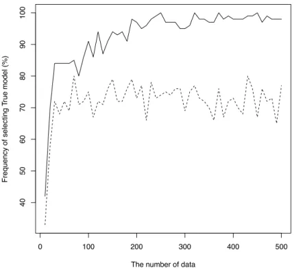
100 samples of two criteria, respectively, to examine the frequency of selecting the true model (see Figure 1). Figure 1 shows that GBIC consistently selects the true model and clearly outperforms DIC as the number of data N increases.
Next we carry out a simulation study to examine the performance of our pro-posed criterion in (2.17) for small sample cases (N = 10,20,30). In this simula-tion, we investigate effects of terms which are discarded as being asymptotically negligible, i.e., log{πk(%θk|ψk)} and log{|J(θ%k)|} in (2.9). We here compare the
0 100 200 300 400 500 40 50 60 70 80 90 100
The number of data
Frequency of selecting T
rue model (%)
Figure 1: Frequency of selecting true model (%) with respect to GBIC and DIC. The solid line indicates GBIC and the dashed line indicates DIC.
the variants of GBIC in (2.9) such as Neath and Cavanaugh (1997) as follows:
GBIC1(y,θ%k) =−2 log{gk(y|%θk)}+dklog(N)
GBIC2(y,θ%k) =−2 log{gk(y|θ%k)}+dklog(N) + log{|J(%θk)|}
where GBIC1 throws out the effects of both log{πk(θ%k|ψk)}and log{|J(%θk)|}such
as BIC proposed by Schwarz (1978) and GBIC2 only throws out the effect of
log{πk(%θk|ψk)}. Notice that Neath and Cavanaugh (1997) evaluates the effects on
BIC of truncation similarly under the maximum likelihood estimation. We also carry out the variable selection using AIC and BIC, which only deal with the
mod-els estimated by the maximum likelihood estimation, to compare the performance of AIC and BIC with that of GBIC.
In this simulation study, we set the true model y = 1.0x1+ 2.0x2+ε, where ε ∼ N(0N,0.5IN) to examine the performance of variable selection and also set
the hyper-parameters in the natural conjugate priors in (2.11) and (2.12) such as b0 = 0K, B0 = κ0IK (κ0 = 1 or 100), ν0 = 0.1, and λ0 = 0.1. We here
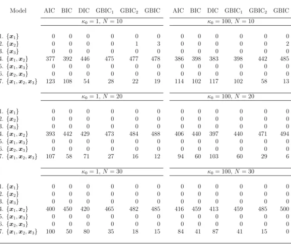
generate 500 samples of each criteria for the seven candidate models and report the frequency of selecting each candidate model in Table 1.
In the case of hyper-parameter κ0 = 1, GBIC2 and GBIC correctly select the
true model (i.e., Model 4) as compared with the results of the other criteria. On the other hand, Table 1 also shows that AIC frequently selects the full model (i.e., Model 7) in all small sample cases (N = 10,20,30).
In the case of hyper-parameter κ0 = 100, the performance of GBIC is quite
well as compared with those of the other criteria. This result reflects the fact that BIC, GBIC1 and GBIC2 are far from the exact marginal likelihood relative
to GBIC. Hence the terms discarded in the derivation of BIC should improve the performance of variable selection. On the other hand, AIC and DIC have a tendency to select the full model.
5
Conclusion and Discussion
In this paper, we consider variable selection in the Bayesian linear regression model with natural conjugate priors. In recent Bayesian modeling, prior information is aggressively applied to estimate the posterior distributions. For example, prior
Table 1: Frequency of set of variables selected by each criteria in 500 samples for small sample cases (N = 10,20,30) when true set of variables is {x1,x2}.
Model AIC BIC DIC GBIC1 GBIC2 GBIC AIC BIC DIC GBIC1 GBIC2 GBIC
κ0= 1,N= 10 κ0= 100,N= 10 1.{x1} 0 0 0 0 0 0 0 0 0 0 0 0 2.{x2} 0 0 0 0 1 3 0 0 0 0 0 2 3.{x3} 0 0 0 0 0 0 0 0 0 0 0 0 4.{x1,x2} 377 392 446 475 477 478 386 398 383 398 442 485 5.{x1,x3} 0 0 0 0 0 0 0 0 0 0 0 0 6.{x2,x3} 0 0 0 0 0 0 0 0 0 0 0 0 7.{x1,x2,x3} 123 108 54 28 22 19 114 102 117 102 58 13 κ0= 1,N= 20 κ0= 100,N= 20 1.{x1} 0 0 0 0 0 0 0 0 0 0 0 0 2.{x2} 0 0 0 0 0 0 0 0 0 0 0 0 3.{x3} 0 0 0 0 0 0 0 0 0 0 0 0 4.{x1,x2} 393 442 429 473 484 488 406 440 397 440 471 494 5.{x1,x3} 0 0 0 0 0 0 0 0 0 0 0 0 6.{x2,x3} 0 0 0 0 0 0 0 0 0 0 0 0 7.{x1,x2,x3} 107 58 71 27 16 12 94 60 103 60 29 6 κ0= 1,N= 30 κ0= 100,N= 30 1.{x1} 0 0 0 0 0 0 0 0 0 0 0 0 2.{x2} 0 0 0 0 0 0 0 0 0 0 0 0 3.{x3} 0 0 0 0 0 0 0 0 0 0 0 0 4.{x1,x2} 400 450 420 465 482 485 416 459 413 459 485 500 5.{x1,x3} 0 0 0 0 0 0 0 0 0 0 0 0 6.{x2,x3} 0 0 0 0 0 0 0 0 0 0 0 0 7.{x1,x2,x3} 100 50 80 35 18 15 84 41 87 41 15 0
decision making (e.g., Rossi and Allenby, 2003). Bayesian analysis provides a unified and coherent way of thinking about decision problems and how to solve them using data and other information (Geweke, 2005).
In this paper, we first proved and illustrated via simulation that our GBIC-based criterion is consistent under the standard assumptions (see Figure 1). Figure 1 shows diverging asymptotic properties of GBIC and DIC: GBIC consistently selects the true model as the number of data increases, while DIC does not as expected. We then compare performance of the proposed GBIC in small sample cases (see Table 1) relative not only to more traditional AIC, BIC, and DIC, but also to the variants GBIC1and GBIC2to evaluate the effect of the terms discarded
in the derivation of BIC on variable selection in linear regression setting.
Table 1 again shows that striking model selection performance differences be-tween the proposed GBIC and DIC: When the prior is informative with κ0 = 1,
neither GBIC nor DIC can escape the influence of strong prior information when the numbers of sample are so small at N = 10,20, and 30; however, it should be noted that the relative rates of misidentification of GBIC is far smaller than the rates of misidentification of DIC.
On the other hand, when the prior is noninformative with κ0 = 100, GBIC’s rates of misidentification are far smaller than the DIC regardless of the number of samples and the GBIC’s misidentification rates rapidly decrease as the num-ber of samples increases. Although GBIC has a very slight chance of choosing underspecified model {x2} for N = 10 whether the prior is informative or
non-informative, the overall small sample performance comparison clearly shows that GBIC is superior to DIC at least in this linear regression setting.
in small sample cases as expected. Therefore in small sample cases where it is crucial to identify the true model under small sample, GBIC and not its truncated versions, GBIC1 and GBIC2, ought to be used. Overall our GBIC-based criterion
is a useful Bayesian variable selection procedure in both large and small sample cases.
As an important direction for the future research, we would like to extend our proposed criterion to Bayesian econometric demand system models (e.g., Kabe and Kanazawa, 2013). Although such models are extensively used in empirical economic studies and policy decision making, their estimation is always constrained by the limited number - at most monthly, but quite often quarterly or semiannually - of data points and thus model performance comparisons must be carried out in small sample situations.
A
Derivation of Eq. (2.15)
Using a fact that p(θ|y,ψ)∝ g(y|θ)π(θ|ψ), we can rewrite the negative Hessian matrix in (2.6) as J(%θ) = −1 N ∂2log{g(y|θ)π(θ|ψ)} ∂θ∂θ! & & & &θ =θ! =−1 N ∂2log{p(θ|y,ψ)} ∂θ∂θ! & & & &θ =θ! . (A.1)
The logarithmic posterior distribution log{p(θ|y,ψ)} in (A.1) for the Bayesian linear regression model in (2.10) is given from (2.13) and (2.14) as
log{p(θ|y,ψ)}= K 2 logσ −2− σ−2 2 (β−b1) !B−1 1 (β−b1) +2ν1 2 −1 3 logσ−2− λ1 2 σ
−2+{constant term}. (A.2)
where parameter vector θ has the parametersβ and σ−2.
The first derivative of (A.2) with respect to β is given by
∂log{p(θ|y,ψ)} ∂β = ∂ ∂β 9 −σ−2 2 (β−b1) !B−1 1 (β−b1) : =−σ− 2 2 ∂ ∂β ; β!B−11β−β!B−11b1−b!1B−11β+b!1B−11b1 < =−σ− 2 2 ; 2B−11β−2B−11b1+ 0 < =−σ−2B−11 (β−b1) (A.3)
Next we take a first derivative of (A.2) with respect to σ−2 as follows: ∂log{p(θ|y,ψ)} ∂σ−2 = ∂ ∂σ−2 9 K 2 logσ −2 − σ− 2 2 (β−b1) !B−1 1 (β−b1) + 2ν1 2 −1 3 logσ−2−λ1 2 σ −2 : = K 2 1 σ−2 − 1 2(β−b1) !B−1 1 (β−b1) + 2ν1 2 −1 3 1 σ−2 − λ1 2 = -K 2 + ν1 2 −1 . (σ−2)−1− 1 2(β−b1) !B−1 1 (β−b1)− λ1 2 . (A.4)
From (A.3), the second derivative of (A.2) with respect to β is obtained as
∂2log{p(θ|y,ψ)} ∂β∂β! = ∂ ∂β ; −σ−2(β−b1)!B−11 < =−σ−2B−11 (A.5)
and with respect to σ−2 is also given by
∂2log{p(θ|y,ψ)} ∂β∂σ−2 = ∂ ∂σ−2 ; −σ−2B−11 (β−b1) < =−B−11(β−b1). (A.6)
Similarly, from (A.4), we take a second derivative of (A.2) with respect to σ−2
as follows ∂2log{p(θ|y,ψ)} ∂σ−2∂σ−2 = ∂ ∂σ−2 9-K 2 + ν1 2 −1 . (σ−2)−1 −1 2(β−b1) !B−1 1 (β−b1)− λ1 2 : = ∂ ∂σ−2 9-K 2 + ν1 2 −1 . (σ−2)−1 : =− -K 2 + ν1 2 −1 .+ σ−2,−2 (A.7)
and with respect to β! is given by ∂2log{p(θ|y,ψ)} ∂σ−2∂β! = ∂ ∂β! 9-K 2 + ν1 2 −1 . (σ−2)−1 −1 2(β−b1) !B−1 1 (β−b1)− λ1 2 : = ∂ ∂β! 9 −1 2(β−b1) !B−1 1 (β−b1) : =−(β−b1)!B−11 (A.8)
Substituting the posterior modesb1 and (ν1−1)/λ1 into parametersβ andσ−2 in
(A.5), (A.6), (A.7) and (A.8), we have the negative Hessian matrixJ(%θ) expressed by J(%θ) = −1 N − 2 ν1−1 λ1 3 B−11 0K 0! K − +K 2 + ν1 2 −1 , 2ν1−1 λ1 3−2 , (A.9)
where 0K is a K×1 vector whose elements are zero.
B
Fern´
andez et al. (2001)’s lemmas
Lemma B.1.
(i) If the true model MT is nested within or is equal to the candidate model Mr
(i.e., MT ⊆Mr), (y−Xrβ% mle r )!(y−Xrβ% mle r ) N p −→σ2. (B.1) (ii) Assuming β!TX!T(IN −Pr)XTβT N p −→cr ∈(0,∞) (B.2)
that for any model Mr that does not nest MT (i.e., MT *⊂ Mr), where Pr = Xr(X!rXr)−1X!r, we obtain (y−Xrβ% mle r )!(y−Xrβ% mle r ) N p −→σ2+cr. (B.3)
Proof. Let us denotePr =Xr(X!rXr)−1X!r, whereXr is aN×Kr design matrix
of the candidate model Mr ∈ Mand Pr and (IN −Pr) are known to be N ×N
symmetric and idempotent matrices. The residual sum of squares for candidate model Mr is given by (y−Xrβ% mle r )!(y−Xrβ% mle r ) =y!(IN −Pr)y = (XTβT +ε)!(IN −Pr) (XTβT +ε) =ε!(IN −Pr)ε+ 2β!TX!T(IN −Pr)ε+β!TX!T (IN −Pr)XTβT. (B.4)
(i)MT ⊆Mr. We assume that Xr is partitioned as Xr = [XT Zr] whereZr is
aN×Sr matrix of additional explanatory variables. When the true variables XT
is regressed on Xr, we have (X!rXr)−1X!rXT = IKT 0Sr×KT . (B.5)
where 0Sr×KT is a Sr×KT matrix whose elements are zero. Then we notice that
(IN −Pr)XT = 7 IN −Xr(Xr!Xr)−1X!r 8 XT =XT −Xr(Xr!Xr)−1X!rXT
=XT −[XT Zr] IKT 0Sr×KT =0N×KT. (B.6)
From (B.6), the residual sum of squares for candidate model Mr in (B.4) can be
rewritten as (y−Xrβ% mle r )!(y−Xrβ% mle r ) =ε!(IN −Pr)ε+ 2β!TX!T (IN −Pr)ε+β!TX!T (IN −Pr)XTβT =ε!(IN −Pr)ε. (B.7)
Since the expectation of (B.7) is given by
E)(y−Xrβ% mle r )!(y−Xrβ% mle r ) * =E[ε!(IN −Pr)ε] =σ2tr{IN −Pr} = (N−KT −Sr)σ2, (B.8) we have as N → ∞,N −Kr−Sr≈N and (y−Xrβ% mle r )!(y−Xrβ% mle r ) N p −→σ2. (B.9)
(ii) MT *⊂Mr. We suppose that
β!TX!T(IN −Pr)XTβT N
p
and expectation of (B.4) is given by E)(y−Xrβ% mle r )!(y−Xrβ% mle r ) * =E[ε!(IN −Pr)ε] +β!TX!T (IN −Pr)XTβT = (N −Kr)σ2+β!TX!T (IN −Pr)XTβT. (B.11) From (B.10) and (B.11), we have as N → ∞, N −Kr ≈N and
(y−Xrβ% mle r )!(y−Xrβ% mle r ) N p −→σ2+cr. (B.12)
Lemma B.2. If the candidate modelMr nests the true modelMT (i.e.,MT ⊂Mr),
Nlog RSST
RSSr d
−→χ2
Kr−KT, (B.13)
where RSSj is a residual sum of squares obtained by RSSj = (y−Xjβ%
mle
j )!(y−
Xjβ% mle
j ) andχ2Kr−KT is a chi-square distribution with degree of freedom Kr−KT.
References
Aitkin, M. (1991). Posterior bayes factors. Journal of the Royal Statistical Society.
Series B (Methodological), pages 111–142.
Akaike, H. (1973). Information theory as an extension of the maximum likelihood principle. pages 267–281, Akademiai Kiado, Budapest. Second International Symposium on Information Theory.
Amemiya, T. (1985). Advanced econometrics. Harvard university press.
Ando, T. (2007). Bayesian predictive information criterion for the evaluation of hierarchical bayesian and empirical bayes models. Biometrika, 94(2):443–458. Berger, J. O. and Pericchi, L. R. (1996). The intrinsic bayes factor for model
selection and prediction. Journal of the American Statistical Association, 91(433):109–122.
Burnham, K. P. and Anderson, D. R. (2002). Model selection and multimodel
inference: a practical information theoretic approach. Springer(c2002), New
York.
Fern´andez, C., Ley, E., and Steel, M. F. (2001). Benchmark priors for bayesian model averaging. Journal of Econometrics, 100(2):381–427.
Gelfand, A. E. and Dey, D. K. (1994). Bayesian model choice: asymptotics and exact calculations. Journal of the Royal Statistical Society. Series B
Geweke, J. (2005). Contemporary Bayesian econometrics and statistics, volume 537. Wiley. com.
Hirose, K., Kawano, S., Konishi, S., and Ichikawa, M. (2011). Bayesian information criterion and selection of the number of factors in factor analysis models.Journal
of Data Science, 9(2):243–259.
Hurvich, C. M. and Tsai, C. L. (1989). Regression and time series model selection in small samples. Biometrika, 76(2):297–307.
Hurvich, C. M. and Tsai, C. L. (1991). Bias of the corrected aic criterion for underfitted regression and time series models. Biometrika, 78(3):499–509. Kabe, S. and Kanazawa, Y. (2013). Estimating the markov-switching almost ideal
demand systems: a bayesian approach. Empirical Economics (forthcoming). Kass, R. E. and Raftery, A. E. (1995). Bayes factors. The Journal of the American
Statistical Association, 90(430):773–795.
Kawano, S. and Konishi, S. (2009). Nonlinear logistic discrimination via regular-ized gaussian basis expansions. Communications in Statistics - Simulation and
Computation, 38(7):1414–1425.
Konishi, S., Ando, T., and Imoto, S. (2004). Bayesian information criteria and smoothing parameter selection in radial basis function networks. Biometrika, 91(1):27–43.
Kubokawa, T. and Srivastava, M. S. (2010). An empirical bayes information cri-terion for selecting variables in linear mixed models. J. Japan Statist. Soc, 40(1):111–130.
Liang, F., Paulo, R., Molina, G., Clyde, M. A., and Berger, J. O. (2008). Mixtures of g priors for bayesian variable selection. Journal of the American Statistical
Association, 103(481).
Matsui, H., Misumi, T., and Kawano, S. (2013). Model selection criteria for the varying-coefficient modelling via regularized basis expansions. Journal of
Statistical Computation and Simulation, pages 1–10.
Neath, A. A. and Cavanaugh, J. E. (1997). Regression and time series model selection using variants of the schwarz information criterion. Communications
in Statistics-Theory and Methods, 26(3):559–580.
Nishii, R. (1984). Asymptotic properties of criteria for selection of variables in multiple regression. The Annals of Statistics, 12(2):758–765.
O’Hagan, A. (1995). Fractional bayes factors for model comparison. Journal of
the Royal Statistical Society. Series B (Methodological), pages 99–138.
Robert, C. P. and Titterington, D. M. (2002). Discussion of a paper by D.J. Spiegelhalter et al. Journal of the Royal Statistical Society. Series B
(Sta-tistical Methodology), 64(4):621.
Rossi, P. E. and Allenby, G. M. (2003). Bayesian statistics and marketing.
Mar-keting Science, 22(3):304–328.
Santis, F. D. and Spezzaferri, F. (2001). Consistent fractional bayes factor for nested normal linear models. Journal of statistical planning and inference, 97(2):305–321.
Schwarz, G. (1978). Estimating the dimension of a model.Annals of Mathematical
Statistics, 42(3):1003–1009.
Spiegelhalter, D. J., Best, N. G., Carlin, B. P., and van der Linde, A. (2002). Bayesian measures of model complexity and fit. Journal of the Royal Statistical
Society. Series B (Statistical Methodology), 64(4):583–639.
Sugiura, N. (1978). Further analysts of the data by akaike’s information criterion and the finite corrections. Communications in Statistics-Theory and Methods, 7(1):13–26.
van der Linde, A. (2005). Dic in variable selection.Statistica Neerlandica, 59(1):45– 56.
Zellner, A. (1986). On assessing prior distributions and bayesian regression analysis with g-prior distributions. Bayesian inference and decision techniques: Essays