A conditional independence algorithm for learning undirected graphical models

(1)

Contents lists available atScienceDirect

Journal of Computer and System Sciences

www.elsevier.com/locate/jcss

A conditional independence algorithm for learning undirected graphical

models

Christian Borgelt

European Center for Soft Computing, Campus Mieres, Ediﬁcio Cientíﬁco-Tecnológico, c/ Gonzalo Gutiérrez Quirós s/n, 33600 Mieres, Asturias, Spain

a r t i c l e

i n f o

a b s t r a c t

Article history:

Received 13 February 2008

Received in revised form 8 December 2008 Available online 18 May 2009

Keywords: Graphical models Possibilistic network Learning from data Conditional independence test

When it comes to learning graphical models from data, approaches based on conditional independence tests are among the most popular methods. Since Bayesian networks dominate research in this ﬁeld, these methods usually refer to directed graphs, and thus have to determine not only the set of edges, but also their direction. At least for a certain kind of possibilistic graphical models, however, undirected graphs are a much more natural basis. Hence, in this area, algorithms for learning undirected graphs are desirable, especially, since ﬁrst learning a directed graph and then transforming it into an undirected one wastes resources and computation time. In this paper I present a general algorithm for learning undirected graphical models, which is strongly inspired by the well-known Cheng–Bell–Liu algorithm for learning Bayesian networks from data. Its main advantage is that it needs fewer conditional independence tests, while it achieves results of comparable quality.

1. Introduction

Modeling complex domains with graphical models, especially Bayesian networks, has become a popular research area since the 1980s [28,38,25,14,21,17], because it allowed for consistent dependence modeling and efficient reasoning. Applications, in particular of Bayesian network classifiers, can nowadays be found in an abundance of areas, including, for example, areas as diverse as manufacturing [1], steel production [29], telecommunication network diagnosis [23], handwrit-ing recognition [8], object recognition in images [33], articulatory feature recognition [16], gene expression analysis [24], protein structure identification [31], and pneumonia diagnosis [6].

In the 1990s, learning graphical models from data became a main focus of attention [9,34,12,20,10,22] and this research direction still attracts a lot of interest after the turn of the century [36,7,11,4,26,19,32,27,37,5]. Several search strategies and scoring functions, which are the two core ingredients of basically all algorithms for learning graphical models, were developed and applied not only to learning probabilistic graphical models, but also for the somewhat less well-known possibilistic networks [18,2,13,4].

Among such learning algorithms, methods that are based on conditional independence (CI) tests are highly popular [35,10,36,11], because they possess several advantages over other learning methods. For example, they do not restrict the structure of the graphs that can be learned (while other approaches may constrain it to be, for example, a polytree or a graph with nodes having a maximum in-degree) and do not require any prior information about the domain (while the famous K2 algorithm, for example, requires, at least in its basic form, a topological order of the attributes as input). They may even be used to enhance other methods, since they can be used to ﬁnd missing prior information (in [34], for example, conditional independence tests are used to determine the topological order needed by the K2 algorithm).

E-mail address:[email protected].

(2)

Unfortunately, though, conditional independence test approaches are usually developed for directed graphs. To some degree this is understandable, since the set of conditional independence statements that can be represented by undirected graphs is monotonic in the condition sets (that is, if a conditional independence statement holds, expanding its set of conditioning attributes must not invalidate the conditional independence). As a consequence, undirected graphs cannot express certain (in)dependence structures that are fairly common in practice. In particular, they cannot capture a structure in which two variables are independent unconditionally, but become dependent conditional on a third variable, which is typical for a situation in which an effect can be brought about—jointly or independently—by two causes. This restriction is also one of the main reasons for the predominance of Bayesian networks (which, since they are based on directed graphs, allow for capturing such dependence structures) in the research on graphical models.

However, at least for a certain kind of possibilistic networks, which are based on a speciﬁc interpretation of degrees of possibility [4], undirected graphs are a much more natural basis. Of course, if one desires an undirected graphical model, it is always possible to turn a found directed graph into a corresponding undirected one by simply “moralizing” the graph (that is, by adding edges between non-adjacent parents of a node). This may lose independence information, but cannot lead to incorrect models. Nevertheless it is desirable to have methods that can learn undirected graphical models directly. In such algorithms the missing edge directions can be exploited, for example, to avoid certain tests and thus to achieve faster and possibly also more robust learning.

In this paper I present an algorithm for learning undirected graphical models that is strongly inspired by the well-known Cheng–Bell–Liu algorithm for learning Bayesian networks [10,11]. Its main advantage is that it requires fewer conditional independence tests, while it achieves results of comparable quality. This paper is organized as follows: in Sections 2 and 3 I brieﬂy review some basics of CI tests needed in the algorithm and in Section 4 recall the Cheng–Bell–Liu algorithm. In Section 5 I present my algorithm for learning undirected graphical models. Section 6 reviews an approach to evaluate learned possibilistic networks, which is then used in Section 7, where experiments, which compare the results of the two algorithms, are reported. Finally, Section 8 draws conclusion from the discussion.

2. Conditional independence and graphical models

In general, graphical models are based on the idea to exploit the structural similarity of the sets of conditional in-dependence statements that can hold in high-dimensional (probability or possibility) distributions and the sets of (node) separation statements that can hold in (directed or undirected) graphs. To be more speciﬁc, both conditional independence statements and (node) separation statements satisfy the so-called (semi-)graphoid axioms:

Deﬁnition 1.LetV be a set of (mathematical) objects and

(

· ⊥⊥ · | ·

)

a three-place relation of subsets ofV. Furthermore, let

W

,

X

,

Y

,

andZ be four disjoint subsets ofV. Then the four statements symmetry:

(

X

⊥⊥

Y

|

Z

)

⇒

(

Y

⊥⊥

X

|

Z

),

decomposition:

(

W

∪

X

⊥⊥

Y

|

Z

)

⇒

(

W

⊥⊥

Y

|

Z

)

∧

(

X

⊥⊥

Y

|

Z

),

weak union:

(

W

∪

X

⊥⊥

Y

|

Z

)

⇒

(

X

⊥⊥

Y

|

Z

∪

W

),

contraction:

(

X

⊥⊥

Y

|

Z

∪

W

)

∧

(

W

⊥⊥

Y

|

Z

)

⇒

(

W

∪

X

⊥⊥

Y

|

Z

)

are called the semi-graphoid axioms. A three-place relation

(

· ⊥⊥ · | ·

)

that satisﬁes the semi-graphoid axioms for all W

,

X

,

Y

,

andZ is called asemi-graphoid. The above four statements together with

intersection:

(

W

⊥⊥

Y

|

Z

∪

X

)

∧

(

X

⊥⊥

Y

|

Z

∪

W

)

⇒

(

W

∪

X

⊥⊥

Y

|

Z

)

are called thegraphoid axioms. A three-place relation

(

· ⊥⊥ · | ·

)

that satisﬁes the graphoid axioms for all W

,

X

,

Y

,

andZ is called agraphoid.

The rationale underlying graphical models is that the three-place relation named in this deﬁnition may either be interpreted as conditional independence or as separation, thus making it possible to use graphs as a “language” for repre-senting sets of conditional independence statements. If the three-place relation is interpreted as conditional independence,

X

⊥⊥

Y

|

Z means that

∀

x

∈

dom

(

X

)

:

∀

y

∈

dom

(

Y

)

:

∀

z

∈

dom

(

Z

)

:

P

(

X

=

x

,

Y

=

y

|

Z

=

z

)

=

P

(

X

=

x

|

Z

=

z

)

·

P

(

Y

=

y

|

Z

=

z

)

in the probabilistic case and

∀

x

∈

dom

(

X

)

:

∀

y

∈

dom

(

Y

)

:

∀

z

∈

dom

(

Z

)

:

(3)

in the possibilistic case. It is easy to show that the semi-graphoid axioms hold for both probabilistic and possibilistic conditional independence and that the graphoid axioms hold for strictly positive probability measures.

What X

⊥⊥

Y

|

Z means if it is interpreted as a statement about separation (of nodes) in a graph depends on whether

the graph is directed or undirected. If it is undirected, the meaning is simply the following:

Deﬁnition 2.LetG

=

(

V

,

E

)

be an undirected graph and X

,

Y

,

andZ three disjoint subsets of nodes. Z u-separates X and

Y inG, written

X

|

Z

|

Y G, iff all paths from a node in X to a node inY contain a node inZ. A path that contains a node

in Z is calledblocked(by Z), otherwise it is calledactive.

For directed graphs the conditions are slightly more complicated:

Deﬁnition 3.LetG

=

(

V

,

E

)

be a directed acyclic graph andX

,

Y

,

andZ three disjoint subsets of nodes.Z d-separates X and

Y inG

, written

X

|

Z

|

Y _G, iff there isnopath from a node in X to a node inY along which the following two conditions hold:

(1) every node with converging edges either is in Z or has a descendant in Z, (2) every other node is not in Z.

A path satisfying the two conditions above is said to beactive, otherwise it is said to beblocked(by Z).

It is easy to show that bothu-separation andd-separation satisfy the graphoid axioms. Hence one may use an appropri-ate graph to capture the set of conditional independence stappropri-atements that hold in a given distribution.

Deﬁnition 4.Let

(

· ⊥⊥

δ

· | ·

)

be a three-place relation representing the set of conditional independence statements that hold

in a given distribution

δ

over a setU of attributes. A (directed or undirected) graphG

=

(

U

,

E

)

overU is called aconditional dependence graphor adependence mapw.r.t.

δ

, iff for all disjoint subsets X

,

Y

,

Z

⊆

U of attributes

X

⊥⊥

δY

|

Z

⇒

X

|

Z

|

Y G

,

i.e., ifGcaptures byu-separation all (conditional) independences that hold in

δ

and thus represents only valid (conditional) dependences. Similarly,Gis called aconditional independence graphor anindependence mapw.r.t.

δ

, iff for all disjoint subsets

X

,

Y

,

Z

⊆

U of attributes

X

|

Z

|

Y G

⇒

X

⊥⊥

δY

|

Z

,

i.e., ifG captures byu-separation only (conditional) independences that are valid in

δ

.G is said to be aperfect mapof the

conditional (in)dependences in

δ

, if it is both a dependence map and an independence map.

Although the correspondence cannot always be made perfect, it is a very convenient tool. Together with the core theorem of graphical models, which connects conditional independence graphs with decompositions of distributions (factorizations in the case of probability distributions), these definitions are the basis of using graphs to capture essential properties of distributions and to derive consistent and efficient methods for drawing inferences in them. W.r.t. learning graphical models from data, these definitions provide the basis for induction algorithms based on conditional independence tests.

3. Conditional independence tests

The core ingredient of the algorithms for learning graphical models, which I focus on in this paper, is a conditional independence test (CI test for short). Such a test usually consists of a scoring function for assessing the strength of the (con-ditional) dependence of two variables together with a threshold. If the value of the scoring function is below the threshold, the variables are considered to be (conditionally) independent, otherwise they are judged to be (conditionally) dependent. By checking which conditional independences hold, one tries to ﬁnd a suitable conditional independence graph. Which con-ditional independences are tested (it is immediately clear that we cannot perform an exhaustive search) is determined by the search strategy (see Sections 4 and 5).

There is an abundance of possible scoring functions, especially for (conditional) probabilistic (in)dependence. The reason is that apart from standard dependence measures used in classical statistics, basically all measures used in decision tree induction can be transferred and then yield such a scoring function. Even if a measure was originally only intended for assessing the strength of marginal dependence, it can usually be extended to yield a measure for conditional dependence by simply computing its value for each possible instantiation of the conditioning attributes and then aggregating these values in a suitable manner. For example, one of the most common measures for the strength of marginal (probabilistic) dependence isinformation gain,

Igain

(

A

,

B

)

=

i,j pi jlog2 pi j pi.p.j

= −

i pi.log2pi.

+

j pj.

i p_i|jlog2pi|j

(4)

(where AandBare two variables,iand jrange over their respective values,pi j,pi.andp.jare the probabilities of the joint

and individual occurrence of these values, and conditional probabilities are deﬁned in the usual way). It can be extended to conditional information gain as

Igain

(

A

,

B

|

C

)

=

k p..k

i,j p_{i j|k}log₂ pi j|k pi.|kp.j|k

,

that is, by simply summing its value over all possible instantiations of the conditions. (Note that hereCmay be an individual variable or a set of variables; and thenkrefers to individual values or value vectors, respectively.)

For the transfer to the possibilistic case, which is discussed below, it is relevant that information gain may be written conveniently as

Igain

(

A

,

B

)

=

H

(

pA

)

+

H

(

pB

)

−

H

(

pA B

),

where H

(

p

)

= −

_ipilog2pidenotes the well-knownShannon entropyof the probability distributionp.

In order to remove the tendency of information gain to over-assess the strength of dependence of many-valued attributes (which is not a fundamental property, but simply results from the discretization of the—estimated—probability values due to the necessarily limited size of a database to learn from; see [4]), it is often normalized toinformation gain ratio

Igr

(

A

,

B

)

=

Igain

(

A

,

B

)

H

(

pA

)

=

i,jpi jlog2 pi j pi.p.j

−

ipilog2pi

or one of its twosymmetrical forms

Isgr1

(

A

,

B

)

=

Igain

(

A

,

B

)

H

(

pA

)

+

H

(

pB

)

=

−

ipilog2pi

−

jpjlog2pj and Isgr2

(

A

,

B

)

=

Igain

(

A

,

B

)

H

(

pA B

)

=

−

i jpi jlog2pi j

.

Worth mentioning is, of course, also the well-known

χ

2_measure,

χ

2

(

A

,

B

)

=

N..

i,j

(

pi.p.j

−

pi j

)

2 pi.p.j

,

whereN..is the total number of sample cases in the database to learn from. Extended to conditional tests it reads

χ

2

(

A

,

B

|

C

)

=

N..

k p_..k

i,j

(

pi.|kp.j|k

−

pi j|k

)

2 pi.|kp.j|k

.

Other probabilistic dependence measures include, for example, the Gini index or the relief measure (see [4] for details and a more extensive list of measures).

Not surprisingly, there is also a variety of measures for the possibilistic case [2,4]. A fairly well-known example is the so-calledspeciﬁcity gain,

Sgain

(

A

,

B

)

=

nsp

(

π

A

)

+

nsp

(

π

B

)

−

nsp

(

π

A B

).

It is easy to see that it is formed in direct analogy to information gain, with the Shannon entropy of a probability distribution replaced by thenon-speciﬁcitynsp

(

π

)

of a possibility distribution

π

. This non-speciﬁcity is deﬁned as

nsp

(

π

)

=

supE

∈Eπ(E) 0 log2 E∈E

[

π

]

α

(

E

)

d

α

,

where

E

is the set of elementary events underlying the possibility distribution

π

(that is, the set of distinct instantiations of the variable or variables) and

[

π

]

α denotes the indicator function of the

α

-cut of the possibility distribution

π

(that is,

[π]

α

(

E

)

=

1 if

π

(

E

)

α

and

[π]

α

(

E

)

=

0 otherwise).

Other measures include the following, which I used to obtain the experimental results reported in Section 7: in the first place, specificity gain may be normalized in analogy to information gain, which serves the purpose to eliminate or at least reduce a possible tendency to overrate the strength of dependence of many-valued attributes. This leads to the specificity gain ratio,

Sgr

(

A

,

B

)

=

Sgain

(

A

,

B

)

nsp

(

π

A

)

=

nsp

(

π

A

)

+

nsp

(

π

B

)

−

nsp

(

π

A B

)

nsp

(

π

A

)

(5)

Fig. 1.Illustration of the phases of the Cheng–Bell–Liu algorithm.

and twosymmetric speciﬁcity gain ratios, namely

Ssgr1

(

A

,

B

)

=

Sgain

(

A

,

B

)

nsp

(

π

A B

)

and Ssgr2

(

A

,

B

)

=

Sgain

(

A

,

B

)

nsp

(

π

A

)

+

nsp

(

π

B

)

.

By exploiting the fact that information gain can be written in two ways, another possibilistic measure can be derived. It relies on the form that is usually called “mutual information” (even though it is the same measure as information gain, since the formulas are equivalent) and compares the actual joint distribution and a hypothetical independent distribution by computing and summing their pointwise quotients, that is,

dmi

(

A

,

B

)

= −

i,j

π

i jlog2

π

i j min

{

π

i.

,

π

.j

}

,

where

π

i j denotes the degree of possibility of the combination of the ith value of attribute A and the jth value of

at-tributeB. Furthermore,

π

i. and

π

j.denote the marginal degrees of possibility, which result from taking the maximum over

all values of the missing index.

Finally, the

χ

2 _{measure (see above), which computes and sums pointwise squared differences between the actual joint}

distribution and a hypothetical independent distribution, can be transferred to possibility distributions. Thus we obtain the following measure: d_χ2

(

A

,

B

)

=

i,j

(

min

{

π

i.

,

π

.j

} −

π

i j

)

2 min

{

π

i.

,

π

.j

}

.

Other scoring functions, as well as a more extensive discussion of the ideas underlying them, can be found in [4].

All of these (possibilistic) scoring functions can be extended to conditional tests by summing their values over all instan-tiations of the conditioning attributes, weighted with the degree of possibility of the instantiation. This mimics the way in which conditional measures are constructed in the probabilistic case from their marginal counterparts (see above).

A general problem of conditional independence tests is their order, that is, the number of conditioning attributes. Since the data sets that are available in practice are always of limited size, conditional independence tests become quickly unre-liable, the higher their order. Hence algorithms for learning graphical models from data must take care to keep the order of conditional independence tests under control. For example, the Cheng–Bell–Liu algorithm, which is reviewed in the next section, does so by exploiting an already constructed graphical model to determine suitable condition sets. If the occurring condition sets still become too large, it is usually ﬁxed that all conditional independence tests with an order higher than a user-speciﬁed maximum fail.

4. The Cheng–Bell–Liu algorithm

The Cheng–Bell–Liu algorithm [10,11] constructs a Bayesian network from a data set of sample cases. It assumes that the given domain can accurately be modeled by a perfect map, that is, by a directed graph that captures exactly the conditional independences that are present in the probability distribution governing the data generation process. In addition, it assumes that the scoring function used for the conditional independence tests is, in a certain sense, well-behaved. Among other things, this means that the result of a conditional independence test coincides with the actual situation (that is, the test succeeds if and only if the tested pair of attributes is actually (conditionally) independent). In addition, if a condition that is needed for the conditional independence of two attributes is removed, the value of the measure should increase, regardless of what other attributes are present in the conditions. For detailed discussion of the exact assumptions and preconditions underlying the Cheng–Bell–Liu algorithm, see [11].

The Cheng–Bell–Liu algorithm works in four phases (see Fig. 1 for a sketch):

4.1. Drafting

A so-called Chow–Liu tree [15] is built as an initial graphical model. This involves evaluating all possible edges (that is, pairs of attributes) with an (unconditional) independence test. The standard form of the algorithm uses information gain as the scoring function and an independence threshold of about 0.1 bits. Edges (identiﬁed by attribute pairs) having

(6)

a score lower than this threshold are permanently discarded from the construction process, since the incident attributes are considered to be (marginally) independent. The rest form a set of candidate edges, which are weighted with the value of the scoring function. The initial graphical model is then formed by constructing an optimum weight spanning tree with these edge weights.

4.2. Thickening

The candidate edges that were not used for the initial graphical model (that is, are not contained in the constructed spanning tree) are traversed in the order of decreasing score. For each of these edges it is tested whether it may be needed in the graphical model. The test exploits the current graphical model in order to ﬁnd a good set of conditions, namely by selecting the set of adjacent nodes of one attribute that lie on paths leading to the other attribute.

The rationale underlying this scheme is the so-calledlocal Markov propertyof directed conditional independence graphs: an attribute is conditionally independent of all non-descendants given its parents (cf. the notion ofd-separation, deﬁned in Deﬁnition 3, which implies this property in a conditional independence graph). Of course, since the graph is undirected at this point we cannot determine which attribute is a non-descendant of the other, and hence both possibilities may have to be tried (one trial with the neighbors of one attribute, another with the neighbors of the other). In addition, the set of adjacent nodes may not only include parents, but also children. Children are a problem, because in the true graphical

model there may be a so-called v-structureon the path between the nodes (that is, there may be a node at which edges

converge). Including such a node (which may be a child) in the conditions is harmful as it activates the path and thus hinders conditional independence.

Therefore the set of adjacent nodes is reduced iteratively and greedily. In each step the conditioning attribute, which, if removed, lowers the dependence score the most, is discarded. This reduction is carried out until the score falls below the given independence threshold or no removal of a conditioning attribute lowers the score. In the former case, if it occurs in either of the two trials, the attributes of the tested edge are judged to be conditionally independent and the edge is not added to the graphical model. Otherwise it is added.

4.3. Thinning

In the thickening phase a test whether an edge is needed was based on a graph that was possibly still too sparse to reveal the conditional independence of a pair of attributes. This is the case, because not all paths that exist between the two attributes in the true model may have been present at the time of the test (even though they must all be present at the end of the thickening phase, provided the assumptions underlying the algorithm hold [11]). Hence the edges that are present in the graphical model after the thickening phase are traversed again and it is retested whether they are needed.

This test is carried out in two ways: ﬁrst in the way described on the thickening phase (which is the so-called “heuris-tic” form of the test). However, there are certain degenerate cases where this test does not correctly identify an existing conditional independence and thus a superﬂuous edge may not be removed (see [11] for an example). Hence a strict test, which adds the neighbors of the attribute’s neighbors to the condition set (because two adjacent nodes on a path cannot both have v-structures) before this set is reduced, is carried out (this is called the so-called “strict” form of the test).

If any of these tests reveals that two attributes are conditionally independent, the corresponding edge is removed from the graph. It can be shown that the resulting graph is a skeleton for the perfect map describing the domain (that is, it contains exactly the needed edges, only directions are missing)—provided, of course, the underlying assumptions hold.

4.4. Orienting

In the last phase the edges of the graph are directed. This is done in two steps: ﬁrst thev-structures (converging edges) are identiﬁed (black arrows in Fig. 1) and then the remaining edges are oriented (gray arrows in Fig. 1), using rules that

avoid the introduction of v-structures and cycles. (The latter step may be done fully automatically or may be supported

manually, since the v-structures usually do not uniquely determine the direction of all edges and thus human intervention may be advisable.)

In order to ﬁnd the v-structures, all pairs of attributes with common neighbors are traversed and it is determined by a (strict) conditional independence test (as described above), which common neighbors are in the (maximally) reduced set of conditions that render the attributes conditionally independent. Those attributes that are removed from the condition set must be common children (since they do not contribute to rendering the attributes conditionally independent, while ﬁxing parents is essential for achieving conditional independence due to the local Markov property). Hence a v-structure is built with them (that is, the edges are directed towards the common neighbor).

Afterwards other edges may be directed by alternatingly extending directed chains and choosing random directions for edges, the direction of which is not ﬁxed by the v-structures and already extended chains. The rationale underlying this procedure is that extending existing chains is the only way to avoid additional v-structures. Furthermore, cycles must, of course, be avoided.

(7)

Fig. 2.Illustration of the phases of the algorithm for undirected graphs.

5. Learning undirected graphs

It is obvious that one way of constructing an undirected graphical model consists in executing the Cheng–Bell–Liu algo-rithm, which yields a directed graph, and then moralizing the result (that is, adding edges between non-adjacent parents of a node). However, from the above description of the algorithm it is clear that in this case a lot of unnecessary work is done. For example, edges are directed and then their direction is discarded again when the graph is moralized. In the tests whether an edge is needed, it is tried to remove children from the condition sets even though in an undirected graph there is no concept of child or parent. Finally, the “strict” form of a conditional independence test has to add the neighbors of the attribute’s neighbors in order to make sure that all paths are securely blocked, regardless of any possibly existing

v-structures, thus introducing a strong tendency towards conditional independence tests of fairly high order. Hence it is desirable to devise an algorithm that removes this unnecessary work and thus obtains an undirected graphical model faster and possibly also in a more reliable way.

The algorithm I propose works in four phases (see Fig. 2 for a sketch):

5.1. Drafting

This phase is identical to the Cheng–Bell–Liu algorithm, that is, a Chow–Liu tree is formed (that is, an optimum weight spanning tree is constructed from edge weights that represent dependence strengths).

5.2. Thickening

As in the Cheng–Bell–Liu algorithm, the remaining candidate edges (that is, edges with a score above the threshold, but not used in the initial graphical model) are traversed and tested. If the test indicates that they may be needed (because the incident attributes are not conditionally independent given the chosen conditions), they are added to the graphical model.

The difference to the Cheng–Bell–Liu algorithm consists in how the conditional independence tests are executed. The underlying principle is analogous, but exploits the local Markov propertyof undirectedgraphs: an attribute is conditionally independent of any other attribute given its neighbors (cf. the notion ofu-separation, deﬁned in Deﬁnition 2, which implies this property in a conditional independence graph). We may even restrict the set of neighbors to those lying on paths leading to the other attribute (even though this is, strictly speaking, already part of the so-calledglobal Markov property).

Note that there is no need for any (greedy or non-greedy) reduction of the condition set, since we need not take care of children withv-structures. In principle, only a single conditional independence test is needed per edge. However, in order to improve the robustness, but also the eﬃciency of the algorithm, it may be advisable to carry out the alternative test (that is, using the neighbors of the other attribute) if it fails. The reason is that a test may fail, because the current graph is still too sparse and thus not all neighbors that are necessary to render the attributes conditionally independent are already present. If this is the case for one attribute, there is still a chance that the set of neighbors of the other attribute is already complete and thus this test is worthwhile.

Clearly, if the executed test indicates that the attributes arenotconditionally independent given the current graph struc-ture, the edge is added to the graph. Otherwise it is discarded.

5.3. Moralizing

If one assumes that there exists an undirected perfect map of the domain under consideration, the thinning phase (see below) already yields the result. However, this would not be a feasible assumption. Dependence structures that contain (directed) v-structures are much too frequent in practice and unfortunately there is no lossless way of representing v -structures in undirected graphs. Hence simply assuming that there is an undirected perfect map would render the algorithm basically useless for practical purposes.

However, in order to take care of v-structures one only has to connect the parents, that is, one has to moralize the

graph. The reason is that even though the parents are independent given their common ancestors (which may be the empty set), they become dependent once a common child is given. This non-monotone behavior (enlarging the set of conditions destroys a conditional independence) cannot be expressed in undirected graphs (cf. Section 2). Thus one must allow for unrepresented conditional independences. However, this is not too much of a problem, since at least for reasoning purposes an independence map suﬃces—we do not necessarily need a perfect map.

(8)

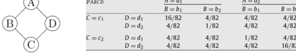
pA BC D A=a1 A=a2 B=b1 B=b2 B=b1 B=b2 C=c1 D=d1 16/82 4/82 4/82 4/82 D=d2 4/82 1/82 4/82 4/82 C=c2 D=d1 4/82 4/82 1/82 4/82 D=d2 4/82 4/82 4/82 16/82 Fig. 3.Example graphical model that can be learned with the proposed algorithm, but not with the Cheng–Bell–Liu algorithm.

The consequences of these considerations for the algorithm are clear: some of the edges, which have an unconditional score below the threshold (and thus were discarded before the initial graphical model was constructed) or were discarded in the thickening phase, may be needed in the graphical model in order to achieve monotony w.r.t. conditional independence. However, for these tests only edges need to be considered that have a common neighbor in the graph constructed so far, since no other edges can connect nodes that are involved in a v-structure. Therefore all such edges are traversed and it is tested whether they are needed in the graph. If the corresponding attributes arenotfound to be conditionally independent given the current graph (that is, given all neighbors of one of the attributes), the edge is added.

5.4. Thinning

As for the Cheng–Bell–Liu algorithm it holds that the graph resulting from the preceding step may contain superﬂuous edges, since when the test was carried out not all necessary edges and paths may have been present in the graph. Hence all edges of the graph are retested and those found to be unnecessary are removed from the graph. (Note that edges added in the thickening step as well as edges added in the moralizing step are retested.)

5.5. Additional thinning

As a simple extension of this algorithm one may add a second thinning phase between the thickening phase and the moralizing phase. The idea of such a phase is that the graph resulting from the thinning phase may contain fewer attribute pairs with common neighbors, so that fewer tests have to be carried out in the moralizing phase. Furthermore, the order of the conditional independence tests may be lower, because a lower number of edges can generally be expected to reduce the number of neighbors that enter the condition sets.

The additional costs for such a phase are negligible, since the results of already executed conditional independence tests will be stored in a cache anyway (to avoid redundant computations). Hence only for edges between attributes that received a new incident edge in the moralizing step a new test has to be carried out in the second thinning phase. The result of all other tests are already present in the cache and thus can be reused basically without costs.

5.6. Illustrative remarks

In order to illustrate the difference of the proposed algorithm to the Cheng–Bell–Liu algorithm, in particular w.r.t. their ability to learn undirected graphical models, consider the example shown in Fig. 3. The (undirected) graph shown on the left is a perfect map of the probability distribution shown on the right. However, the Cheng–Bell–Liu algorithm is unable to discover this graph. The reason is that it makes the assumption that there is a directed perfect map of the domain under consideration. However, there is no directed perfect map for this probability distribution.

Nevertheless, carrying out the Cheng–Bell–Liu algorithm for this probability distribution (or a corresponding data set), and then moralizing the resulting graph, yields a proper undirected independence map of this probability distribution. Unfortunately, though, this map contains a superﬂuous edge, namely either the edge A—C or the edge B—D (which edges is selected depends on the order in which edges with the same score are processed). Note that the thinning phase of the Cheng–Bell–Liu algorithm cannot remove this edge, because it is actually introduced by the moralizing step and not part of the result of the Cheng–Bell–Liu algorithm (which contains an (incorrect) v-structure).

This example also reveals that using the Cheng–Bell–Liu algorithm to learn an undirected graphical model may fail to ﬁnd the best undirected graphical model even if there exists an undirected perfect map of the domain and thus provides an additional argument in favor of the proposed algorithm. This algorithm ﬁnds the optimal model easily, since it is already the result of the thickening phase, and neither moralizing nor thinning change the graph.

6. Possibilistic network evaluation

The measures studied in Section 3 are local evaluation measures, because they only assess the strength of dependence of two attributes, possibly given a set of conditioning attributes. However, in order to evaluate a learned network, we need a global evaluation measure that considers the network as a whole. The idea underlying such a measure is that in order to assess a possibilistic graphical model, we may compare the possibility distribution represented by it to the one that is induced by the dataset to learn from.

(9)

The problem with this approach is, of course, that in order to do so, we would have to compute the degrees of possibility for all points of the multidimensional domain. This is clearly impossible, though, unless there are very few attributes: the size of this joint domain grows exponentially with the number of attributes.

However, we may consider restricting the set of points from which we compute this measure, so that the computation becomes eﬃcient. If we select a proper subset of points of the underlying multidimensional domain, the resulting ranking of different graphical models may coincide with the ranking computed from the full set of points.

A natural choice for such a subset is the set of sample cases recorded in the dataset to learn from, because from these the distribution is induced and thus it is most important to approximate their degrees of possibility well. In addition, we may weight the degrees of possibility for these sample cases with their frequency in order to capture their relative importance. That is, we may compute

Q

(

G

)

=

t∈D

w

(

t

)

· π

G

(

t

),

to assess the quality of a given graphical modelG [4], where D is the dataset to learn from and w

(

t

)

is the weight of a tuplet (basically: its number of occurrences in the data). This measure should be minimized by a learning algorithm, since a bad graphical model will, on average, assign higher degrees of possibility than a good one. The reason is that the degrees of possibility of the distribution represented by the graphical model are computed as minima of maximum projections that were derived from the dataset. Therefore these degrees of possibility can only be greater than the degrees of possibility of the induced possibility distribution, but never smaller. Only if the graphical model represents the database-induced possibility distribution perfectly, these degrees of possibility are equal. Consequently, we should strive to make the degrees of possibility that are computed from the graphical model as small as possible, in order to approximate the database-induced possibility distribution as closely as possible.

Of course, computing the value of the above measure is simple only if all tuples are precise (that is, if there are no miss-ing values or imprecise information about attribute values), because only for a precise tuple a unique degree of possibility can be determined from the graphical model to evaluate. For an imprecise tuple (with missing values or sets of alternative values) some kind of approximation has to be used. We may, for instance, compute an aggregate, e.g. the average or the maximum, of the degrees of possibility of all precise tuples that are compatible with an imprecise tuple. Since we are trying to minimize the value of the measure, it seems natural to choose pessimistically the maximum as the worst possible case. This choice has the additional advantage that it can be computed eﬃciently by simply propagating the evidence contained in an imprecise tuple in the given graphical model, whereas other aggregates suffer from the fact that we have to compute explicitly the degree of possibility of every compatible precise tuples. Because the number of these tuples can be very large, such an evaluation can be extremely costly.

7. Experiments

In order to test the learning algorithm proposed above, I implemented it as part of the INeS program (Induction of Network Structures), which also comprises a large number of other learning algorithms for probabilistic and possibilistic graphical models, including the Cheng–Bell–Liu algorithm.1

As a ﬁrst test case I chose a standard benchmark, namely the well-known BOBLO (BOvine BLOod) network and data set [30], which is also known as the Danish Jersey cattle data. It consists of a manually constructed Bayesian network over 21 attributes, which describe genotypical and phenotypical properties of dam, sire and calf, together with switch variables that specify whether dam and sire were correctly identiﬁed. The network serves the purpose to verify parentage for pedigree registration. In addition, there is a real-world data set of 500 cases, a large number of which contain missing values.

I focused on learning a possibilistic network, since at least the kind, in which conditional distributions are identiﬁed with joint distributions on the same subspace, is more naturally represented with the help of an undirected graph. In the imple-mentation I made use of a method to eﬃciently compute maximum projections of a multivariate possibility distribution [3], which is represented by a database of sample cases with missing values or set-valued information.

As already pointed out in Section 3, I collected scoring functions from [2,4], taking the restriction into account that the measure must be symmetric in order to be usable for a conditional independence test. As a consequence I chose the speci-ﬁcity gain Sgain, a symmetric ratio of the speciﬁcity gain Ssgr1 (the two variants mentioned in Section 3 behave similarly),

the possibilistic analog of the

χ

2_measure_d

χ2, and the possibilistic analog of mutual informationdmi (see Section 3 for the

deﬁnitions). As independence thresholds I used 0.015 for Sgain, 0.1 for Ssgr1 anddχ2, and 0.04 fordmi. These values were

chosen, because they yielded reasonably good results. By tuning these values, the complexity of the learned network may be controlled to some degree: the higher the threshold, the sparser the learned network.

The results of the experiments together with information about the number of conditional independence tests needed are shown in Tables 1 and 2. Table 1 shows the size and the quality of the networks learned with the Cheng–Bell–Liu

1 _{Note, however, that [10,11] do not specify all relevant details of the algorithm. Especially, there is no clear description how cycles introduced by}

v-structures—a situation that can occur due to certain numerical properties of information gain in connection with a threshold—are treated. Hence INeS may produce results that differ from the reference implementation of this algorithm.

(10)

Table 1

Network quality with Cheng–Bell–Liu algorithm (and moralization), BOBLO data.

Measure Edges Params Min. Avg. Max.

Sgain 16 678 8.738 8.886 10.614

Ssgr1 20 4701 8.638 8.826 10.340

dχ2 14 9450 9.344 9.446 10.728

dmi 17 1010 8.460 8.538 10.406

Table 2

Network quality of learning an undirected graphical model, BOBLO data.

Sgain 17 639 8.738 8.888 10.614

Ssgr1 21 3847 8.740 8.926 10.464

d_χ2 12 3442 9.352 9.453 10.730

dmi 19 570 8.586 8.656 10.558

Table 3

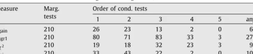
Number of tests with strict Cheng–Bell–Liu algorithm, BOBLO data. Measure Marg.

tests

Order of cond. tests

1 2 3 4 5 any Sgain 210 26 23 13 2 0 64 Ssgr1 210 79 77 86 33 3 278 dχ2 210 20 20 36 24 3 103 dmi 210 28 46 43 9 0 126 Table 4

Number of tests with heuristic Cheng–Bell–Liu algorithm, BOBLO data. Measure Marg.

tests

1 2 3 4 5 any

Sgain 210 26 23 13 2 0 64

Ssgr1 210 80 71 83 33 3 270

dχ2 210 19 18 32 23 3 95

dmi 210 33 43 22 2 0 100

algorithm and subsequent moralization using different scoring functions. The number of edges (in the moralized graph) and the number of parameters show the considerably different behavior of the measures w.r.t. the complexity of the learned network. The last three columns state the sums of the minimum, average, and maximum possibility degree of points covered by the tuples in the database, which should be as low as possible (see Section 6 for a description of how these values are computed).

As could also be observed in experiments with other learning algorithms,d_χ2 tends to learn large networks. However,

they are usually of better quality than the ones built by the Cheng–Bell–Liu algorithm. This could not be improved by increasing the independence threshold: although the networks get smaller when doing so, they also get even worse, thus indicating that this measure may not be well suited for an approach based on conditional independence tests. With the pos-sibilistic analog of mutual informationdmi and the speciﬁcity gainSgain, however, results are obtained that are competitive

with other learning approaches. This conﬁrms earlier results (see [4]) thatdmi is among the most recommendable measures

for learning possibilistic graphical models.

Table 2 shows the results for the proposed algorithm that learns undirected graphical models directly. It can be observed that it tends to learn smaller networks: even though the number of edges is the same or even slightly larger, the number of parameters is clearly smaller for all measures. Nevertheless the quality of the learned networks is comparable, only for

dmi the quality deteriorates slightly. However, this may be counteracted by adapting the independence threshold (a smaller

threshold improves the network quality).

My main goal when developing the proposed algorithm was to reduce the number of the conditional independence tests, especially of higher order. Therefore Tables 3 to 5 show the number of (conditional) independence tests that were carried out by the two algorithms. Since the drafting phase is identical in both algorithms, they execute the same number of marginal independence test, namely 210 (

=

21₂·20). This number obviously cannot be reduced, since all edges must be tested marginally. However, there are considerable differences in the number of conditional independence tests carried out. In order to treat the original Cheng–Bell–Liu algorithm as fairly as possible, I executed it in two versions. The ﬁrst version is the one as it was described above and the numbers of tests needed are shown in Table 3. The second version is simpliﬁed in as far as in the thinning phase it only carries out heuristic tests (using only direct neighbors in the condition sets) and skips the strict tests (using also neighbors of neighbors). Both versions lead to the same networks on this example

(11)

Table 5

Number of tests with algorithm for undirected graphs, BOBLO data. Measure Marg.

tests

1 2 3 4 5 any Sgain 210 13 11 5 4 0 33 Ssgr1 210 42 29 16 3 0 90 d_χ2 210 9 7 2 8 0 26 dmi 210 13 15 20 0 0 48 Table 6

Network quality with Cheng–Bell–Liu algorithm (and moralization), Monk data.

Sgain 4 232 3.401 3.806 4.253

Ssgr1 5 131 3.970 4.287 4.616

dχ2 6 240 3.378 3.777 4.211

dmi 4 232 3.401 3.806 4.253

Table 7

Network quality of learning an undirected graphical model, Monk data.

Sgain 5 145 3.953 4.256 4.579

Ssgr1 5 131 3.970 4.287 4.616

dχ2 7 153 3.912 4.210 4.522

dmi 5 145 3.953 4.256 4.579

problem and thus Table 1 applies for both version. However, in terms of the number of conditional independence tests one can expect fewer and lower order tests with the second version. This is conﬁrmed by Table 4, although the gains are a lot smaller than I had expected. The reason may be that for the orienting phase strict tests are needed anyway and thus skipping them in the thinning phase does not help much. The biggest savings result fordmi, where the number of tests goes

down by 26.

In contrast to these fairly small gains the gains achieved by using the proposed algorithm for learning undirected graphs directly are considerable. The number of conditional independence tests is cut to about half of the tests needed by the Cheng–Bell–Liu algorithm. The biggest gains result ford_χ2, but alsod_mi, one of the most recommendable measure, beneﬁts

signiﬁcantly. It is worth noting that for all measures exceptSgainthe highest order of a conditional independence test drops

by 1.

As a second test to confirm these results I ran experiments on the well-known Monk data sets, which are three artifi-cial data sets encoding certain deterministic relations between six many-valued attributes and a binary class attribute. In order to make these data sets suitable for possibilistic network learning, 10% of missing values where randomly inserted into each data set. From these modified data sets the networks where then induced. Like for the BOBLO data, the indepen-dence thresholds where adapted (to somewhat lower values than for the BOBLO data) so that the network induction yields plausible results.

Since the results are fairly similar on the three data sets, I only report the results on the second here. The assessment of the network quality of the learned networks is shown in Table 6 for the Cheng–Bell–Liu algorithm and in Table 7 for the algorithm proposed in this paper. Clearly, there is a strong relationship between the number of parameters and the network quality: the more complex the network (in terms of the number of parameters), the worse its evaluation. However, this can, in principle, be counteracted by adapting the independence threshold. Here I refrained from doing so, because the quality is still acceptable and the lower complexity may even be seen as an advantage.

The number of conditional independence tests needed to learn the networks with the different conditional independence test measures is shown in Table 8 to 10. Clearly, the general impression is the same as for the BOBLO data: the number of needed conditional independence tests is considerably reduced, in one case even removing the necessity of a test of third order. It has to be considered, though, that here this gain comes at a somewhat stronger deterioration in terms of the network quality.

Similar results are obtained for the other two monk data sets: at the price of a slightly lower network quality, networks of lower complexity are obtained with considerably fewer conditional independence tests.

8. Conclusions

In this paper I presented an algorithm for learning undirected graphical models from data that is based on condi-tional independence tests and inspired by the well-known Cheng–Bell–Liu algorithm. It is particularly useful for possibilistic networks, since at least for a certain kind of these networks undirected graphs are the most natural representation. The expectation that the algorithm would achieve its results with fewer conditional independence tests or conditional

(12)

indepen-Table 8

Number of tests with strict Cheng–Bell–Liu algorithm, Monk data. Measure Marg.

tests

1 2 3 any Sgain 21 20 24 8 52 Ssgr1 21 18 15 3 36 d_χ2 21 19 24 8 51 dmi 21 19 24 8 51 Table 9

Number of tests with heuristic Cheng–Bell–Liu algorithm, Monk data. Measure Marg.

tests

1 2 3 any Sgain 21 19 22 7 48 Ssgr1 21 18 15 3 36 dχ2 21 18 22 7 47 dmi 21 19 22 7 48 Table 10

Number of tests with algorithm for undirected graphs, Monk data. Measure Marg.

tests

1 2 3 any

Sgain 21 4 5 7 16

Ssgr1 21 5 6 0 11

dχ2 21 4 5 7 16

dmi 21 5 5 7 16

dence tests of lower order was clearly conﬁrmed in the reported experiments. Hence if undirected graphical models are to be learned, the presented algorithm provides signiﬁcant advantages. It may be conjectured that it is not only faster, but also provides more reliable results, since the number and order of the tests is decisive in this respect. However, this needs to be substantiated with more experiments.

8.1. Software

The INeS program, which is written in C and was used to carry out the experiments described above, can be downloaded

free of charge at

http://www.borgelt.net/ines.html

.

References

[1] J.M. Agosta, Intel Technol. J. 8 (4) (2004) 361–372, Intel Corporation, Santa Clara, CA, USA.

[2] C. Borgelt, R. Kruse, Evaluation measures for learning probabilistic and possibilistic networks, in: Proc. 6th IEEE Int. Conf. on Fuzzy Systems, vol. 2, FUZZ–IEEE’97, Barcelona, Spain, IEEE Press, Piscataway, NJ, USA, 1997, pp. 1034–1038.

[3] C. Borgelt, R. Kruse, Eﬃcient maximum projection of database-induced multivariate possibility distributions, in: Proc. 7th IEEE Int. Conf. on Fuzzy Systems, FUZZ–IEEE’98, Anchorage, Alaska, USA, IEEE Press, Piscataway, NJ, USA, 1998 (CD-ROM).

[4] C. Borgelt, R. Kruse, Graphical Models — Methods for Data Analysis and Mining, J. Wiley & Sons, Chichester, United Kingdom, 2002.

[5] G. Castillo, Adaptive learning algorithms for Bayesian network classiﬁers, AI Commun. 21 (1) (2008) 87–88, IOS Press, Amsterdam, Netherlands. [6] T. Charitos, L.C. van der Gaag, S. Visscher, K.A.M. Schurink, P.J.F. Lucas, A dynamic Bayesian network for diagnosing ventilator-associated pneumonia in

ICU patients, Expert Systems Appl. 36 (2.1) (2007) 1249–1258, Elsevier, Amsterdam, Netherlands.

[7] D.M. Chickering, Optimal structure identiﬁcation with Greedy search, J. Mach. Learn. Res. 3 (2002) 507–554, MIT Press, Cambridge, MA, USA. [8] S.-J. Cho, J.H. Kim, Bayesian network modeling of strokes and their relationship for on-line handwriting recognition, Pattern Recogn. 37 (2) (2003)

253–264, Elsevier Science, Amsterdam, Netherlands.

[9] G.F. Cooper, E. Herskovits, A Bayesian method for the induction of probabilistic networks from data, Mach. Learn. 9 (1992) 309–347, Kluwer, Dordrecht, Netherlands.

[10] J. Cheng, D.A. Bell, W. Liu, Learning belief networks from data: An information theory based approach, in: Proc. 6th ACM Int. Conf. Information Theory and Knowledge Management, CIKM’97, Las Vegas, NV, ACM Press, New York, NY, USA, 1997, pp. 325–331.

[11] J. Cheng, R. Greiner, J. Kelly, D.A. Bell, W. Liu, Learning Bayesian networks from data: An information theory based approach, Artiﬁcial Intelli-gence 137 (1–2) (2002) 43–90, Elsevier, Amsterdam, Netherlands.

[12] W. Buntine, Operations for learning with graphical models, J. Artiﬁcial Intelligence Res. 2 (1994) 159–225, Morgan Kaufman, San Mateo, CA, USA. [13] L.M. de Campos, J.F. Huete, S. Moral, Independence in uncertainty theories and its application to learning belief networks, in: D. Gabbay, R. Kruse

(Eds.), DRUMS Handbook on Abduction and Learning, Kluwer, Dordrecht, Netherlands, 2000, pp. 391–434.

[14] E. Castillo, J.M. Gutierrez, A.S. Hadi, Expert Systems and Probabilistic Network Models, Springer, New York, NY, USA, 1997.

[15] C.K. Chow, C.N. Liu, Approximating discrete probability distributions with dependence trees, IEEE Trans. Inform. Theory 14 (3) (1968) 462–467, IEEE Press, Piscataway, NJ, USA.

[16] J. Frankel, M. Webster, S. King, Articulatory feature recognition using dynamic Bayesian networks, Comput. Speech and Lang. 21 (4) (2007) 620–640, Elsevier Science, Amsterdam, Netherlands.

(13)

[17] J.A. Gamez, S. Moral, A. Salmeron, Advances in Bayesian Networks, Springer, Berlin, Germany, 2004.

[18] J. Gebhardt, Learning from data: Possibilistic graphical models, Habilitation Thesis, University of Braunschweig, Germany, 1997.

[19] Learning Bayesian network classiﬁers by maximizing conditional likelihood, in: Proc. 21st Int. Conf. on Machine Learning, ICML 2004, Banff, Alberta, Canada, ACM Press, New York, NY, USA, 2004, p. 46.

[20] D. Heckerman, D. Geiger, D.M. Chickering, Learning Bayesian networks: The combination of knowledge and statistical data, Mach. Learn. 20 (1995) 197–243, Kluwer, Dordrecht, Netherlands.

[21] F.V. Jensen, Bayesian Networks and Decision Graphs, Springer, Berlin, Germany, 2001. [22] M.I. Jordan (Ed.), Learning in Graphical Models, MIT Press, Cambridge, MA, USA, 1998.

[23] R.M. Khanafar, B. Solana, J. Triola, R. Barco, L. Moltsen, Z. Altman, P. Lazaro, Automated diagnosis for UMTS networks using a Bayesian network approach, IEEE Trans. Veh. Technol. 57 (4) (2008) 2451–2461, IEEE Press, Piscataway, NJ, USA.

[24] S. Kim, S. Imoto, S. Miyano, Dynamic Bayesian network and nonparametric regression for nonlinear modeling of gene networks from time series gene expression data, Biosystems 75 (1–3) (2004) 57–65, Elsevier Science, Amsterdam, Netherlands.

[25] S.L. Lauritzen, Graphical Models, Oxford University Press, Oxford, United Kingdom, 1996. [26] R.E. Neapolitan, Learning Bayesian Networks, Prentice Hall, Englewood Cliffs, NJ, USA, 2004.

[27] R.S. Niculescu, T.M. Mitchell, R.B. Rao, Bayesian network learning with parameter constraints, J. Mach. Learn. Res. 7 (2006) 1357–1383, Microtome Publishing, Brookline, MA, USA.

[28] J. Pearl, Probabilistic Reasoning in Intelligent Systems: Networks of Plausible Inference, Morgan Kaufmann, San Mateo, CA, USA, 1988 (2nd edition, 1992).

[29] F. Pernkopf, Detection of surface defects on raw steel blocks using Bayesian network classiﬁers, Pattern Anal. Appl. 7 (3) (2004) 333–342, Springer, London, United Kingdom.

[30] L.K. Rasmussen, Blood Group Determination of Danish Jersey Cattle in the F-blood Group System, Dina Res. Rep., vol. 8, Dina Foulum, Tjele, Denmark, 1992.

[31] V. Robles, R. Larrañaga, J. Pena, E. Menasalvas, M. Perez, V. Herves, A. Wasilewska, Bayesian network multi-classifiers for protein secondary structure identification, Artificial Intelligence Med. 31 (2) (2004) 117–136, Elsevier Science, Amsterdam, Netherlands.

[32] T. Roos, H. Wettig, P. Grünwald, P. Myllymäki, H. Tirri, On discriminative Bayesian network classiﬁers and logistic regression, Mach. Learn. 65 (1) (2005) 31–78, Springer, Amsterdam, Netherlands.

[33] H. Schneiderman, Learning a restricted Bayesian network for object recognition, in: Proc. IEEE Conf. on Computer Vision and Pattern Recognition, CVPR’04, Washington, DC, IEEE Press, Piscataway, NJ, USA, 2004, pp. 639–646.

[34] M. Singh, M. Valtorta, An algorithm for the construction of Bayesian network structures from data, in: Proc. 9th Conf. on Uncertainty in Artiﬁcial Intelligence, UAI’93, Washington, DC, USA, Morgan Kaufmann, San Mateo, CA, USA, 1993, pp. 259–265.

[35] P. Spirtes, C. Glymour, R. Scheines, Causation, Prediction, and Search, Lecture Notes in Statist., vol. 81, Springer, New York, NY, USA, 1993. [36] H. Steck, Constraint-based structural learning in Bayesian networks using ﬁnite data sets, PhD thesis, TU München, Germany, 2001.

[37] I. Tsamardinos, L.E. Brown, C.F. Aliferis, The max–min Hill-Climbing Bayesian network structure learning algorithm, Mach. Learn. 65 (1) (2006) 31–78, Springer, Amsterdam, Netherlands.