© 2016 IEEE. Personal use of this material is permitted. Permission from IEEE must be obtained for
all other uses, in any current or future media, including reprinting/republishing this material for
advertising or promotional purposes, creating new collective works, for resale or redistribution to
servers or lists, or reuse of any copyrighted component of this work in other works.
Local Depth Patterns for
Fine-Grained Activity Recognition in Depth Videos
Sari Awwad
Global Big Data Technologies Centre Faculty of Engineering and IT University of Technology Sydney Email: [email protected]
Massimo Piccardi
Global Big Data Technologies Centre Faculty of Engineering and IT University of Technology Sydney Email: [email protected]
Abstract—Fine-grained activities are human activities involv-ing small objects and small movements. Automatic recognition of such activities can prove useful for many applications, including detailed diarization of meetings and training sessions, assistive human-computer interaction and robotics interfaces. Existing approaches to fine-grained activity recognition typically leverage the combined use of multiple sensors including cameras, RFID tags, gyroscopes and accelerometers borne by the monitored people and target objects. Although effective, the downside of these solutions is that they require minute instrumentation of the environment that is intrusive and hard to scale. To this end, this paper investigates fine-grained activity recognition in a kitchen setting by solely using a depth camera. The primary contribution of this work is an aggregated depth descriptor that effectively captures the shape of the objects and the actors. Experimental results over the challenging “50 Salads” dataset of kitchen activities show an accuracy comparable to that of a state-of-the-art approach based on multiple sensors, thereby validating a less intrusive and more practical way of monitoring fine-grained activities.
Index Terms—Index Terms: Fine-grained activity recognition, local depth descriptors, M-SVM2 classifier, “50 Salads” activity
recognition dataset.
I. INTRODUCTION
The main aim of fine-grained activity recognition is to correctly identify activities of limited inter-class variance, often involving small objects and short-range movements. The automated recognition of such activities can play an important role in real-life applications such as the automated diarization of events, including meetings and training sessions, the verifi-cation of compliance to protocols and procedures, and human-robot interaction [1]–[3]. Typical approaches to fine-grained activity recognition leverage a variety of embedded sensors such as RFID tags, gyroscopes, and accelerometers attached to the body of the agents and to selected, target objects [4]. These sensors are often complemented by cameras to help with the fine localization of objects and the measurement of gestures and movements [5], [6]. In addition, inexpensive depth cameras such as Play Station Eye and Microsoft Kinect have made depth videos widely available and easily usable for this task.
Despite the progress in this area, the use of multiple sensors poses practical limitations to the applicability of this
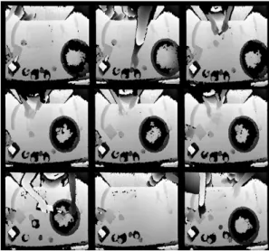
technol-ogy. As a matter of fact, the requirement of equipping people and target objects with borne sensors may prove cumbersome or impractical in many scenarios. The use of borne sensors also makes it possible to identify their carrier by association, which may not be desirable in cases where privacy is paramount. For these reasons, in this short paper we present an approach to fine-grained activity recognition that solely leverages the use of a depth camera. Depth images do not depict sig-nificant personal traits of the viewed subjects and therefore are substantially privacy-preserving. The approach is applied to a kitchen scenario where only a single camera is placed unobtrusively above the cooking plane, without interfering with the actions and with no additional instrumentation. The dataset used for the experiments is the challenging “50 Salads” dataset which was released as part of a recent publication to offer a unified and probing benchmark for fine-grained activity recognition from RGB, depth and accelerometric data [4]. Figure 1 shows an example of depth frames from this dataset. The experimental results in Section IV show that the proposed approach is capable of achieving an accuracy comparable to that of a state-of-the-art method that uses both cameras and accelerometers, making it possible to apply fine-grained activity recognition in a wide range of scenarios.
Fig. 1. Examples of depth frames from the “50 Salad” dataset. 978-1-5090-2748-4/16/$31.00 2016 IEEE
II. RELATEDWORK
The two main, interrelated issues in fine-grained activity recognition are the localization of the objects and parts of interest, and the characterization and modelling of their shape and movement [7]. Accordingly, the related work is organized over two subsections concerning object localization and fea-ture vectors.
A. Object Localization
Previous research on object localization has exploited the use of attached instrumentation such as RFID tags and ac-celerometers to locate the objects of interest. Such sensors are often used in conjunction with video cameras, so that the localization accuracy can be increased by aligning their data with the video data [2], [4], [8]–[12]. The training of these combined approaches require annotation of the “bounding boxes” of the objects in the visual data, and synchronization with the sensor data. Other approaches are based on active learning and require further human intervention during the system’s training: for instance, [12] required the use of user clicks as a means of guiding the machine toward correct identification; [13] exploited online supervision to improve the model; and [14] assumed knowledge of the true position of parts at run time. To relax the requirements on video annotation, [1] has recently proposed searching the Web for “highlights” of the objects of interest. However, this approach is heavily affected by the inaccuracy of the search results. To the best of our knowledge, [15] is the only work to date to have addressed fine-grained activity recognition without any annotation of the frames. However, it only addresses recognition in still images, rather than in live settings as in the scope of this work.
B. Feature Vectors
The use of video data requires the design of effective descriptors of the activities. While it is possible, in prin-ciple, to use precise geometric models of the objects and the agents as descriptors, their fitting onto the video data often fails due to the cluttering in the environment and the limited resolution of the video frames. For this reason, the mainstream trend in recent years has been to use a variety of local features, i.e. compound descriptors of image patches which are mildly invariant to artifacts such as illumination and viewpoint changes [16]. A great deal of local features have been proposed, including, but not limited to, spatio-temporal interest points (SIFT), speeded-up robust features (SURF), and local binary patterns (LBP) [17]–[19] which have proved effective not only for activity recognition, but also for object detection and tracking. In addition, the recent advent of consumer depth cameras has led to the proposal of many depth-based local features aimed at encapsulating the local 3D shape of objects. For instance, [20] has proposed the HON4D feature, a histogram of oriented 4D normals suitable for recognizing activities from depth video. Xia and Aggarwal in [21] have proposed a depth-based modification of the popular STIP detector and descriptor, and [22] has
proposed a combination of RGB and depth features. However, local features for fine-grained activity recognition in depth videos still constitute a subject of investigation [23].
III. PROPOSEDAPPROACH
In this paper, we show how depth videos alone enable an accurate solution to fine-grained activity recognition. This approach is demonstrated in a kitchen environment where various actors attend to the preparation of mixed salads in a spontaneous and realistic way. Figure 2 shows an overview of the proposed approach, while the remainder of this section describes the main components.
LDPT feature extraction Fisher vector encoding M-SVM2 multi-class multi-classification
Fine-grained activity label
Input frames
Fig. 2. Overview of the proposed approach.
A. The Local Depth Feature: LDPT
Local video features have proved versatile over diverse tasks such as activity recognition, detection and tracking. In [24], the authors have proposed a local depth feature for tracking (LDPT) that has ranked highly in a challenging tracking benchmark of depth videos. Since the feature has proved able to represent the target shape under mild deformations and viewpoint changes, we believe that it could also be effective for representing the shape of the objects of interest in fine-grained activity recognition. For this reason, we choose an appropriate size for the LDPT feature and we partition each depth frame into a grid of non-overlapping LDPTs with H rows and V columns. While the use of overlap between adjacent LDPTs can soften boundary effects, we found it was not beneficial in practice.
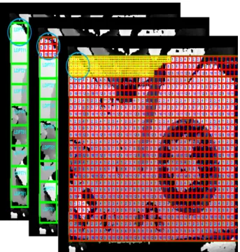
The LDPT, in turn, consists of anHD×V D grid of “depth patterns” (DP) [23] that encapsulate the directional derivatives within a small square patch. Each depth pattern first sub-divides its square patch into 3×3 cells, and then computes the absolute differences between the average depth of every pair, saving these differences in a 3∗23 = 36-dimensional vector. For clarity, Figure 3 shows the hierarchy of the cells,
Fig. 3. The hierarchy of cells (smallest), depth patterns (intermediate; numbered from1to12) and LDPTs (largest). This figure should be viewed in color.
depth patterns and LDPTs. Algorithm 1 shows the detailed steps for computing an LDPT feature.
Algorithm 1 The algorithm for computing an LDPT feature. Input: Depth frame region
Output: LDPT feature
1: LDP T =nil 2: loop r = 1 : VD
3: loop c = 1 : HD
4: DP(r, c) =nil
{computes the difference between every cell pair:} 5: loop k = 1 : 9
6: loop j = k + 1 :9
7: dif f(k, j) =|avgdepth(k)−avgdepth(j)| DP(r, c) =concatenate(DP(r, c), dif f(k, j)) 8: end loop 9: end loop LDP T =concatenate(DP(r, c)) 10: end loop 11: end loop B. Feature Encoding
After the completion of the feature extraction stage, the local features of each frame are encoded into a more compact and descriptive representation called an encoding. Encodings are a key component of visual recognition algorithms, with the most popular being the bag-of-features, the vector of locally aggregated descriptors (VLAD) and the Fisher vector [25]– [27]. In [15], the authors have shown that the Fisher vector is
especially suitable for the recognition of fine-grained activities, thanks to its ability to retain detailed information. Given a Gaussian mixture model (GMM) withMdiagonal components and parameters {wm, µm, σm, m = 1. . . M} (respectively, weight, mean and standard deviation of them-th component), the Fisher vector encodes a set of local features,X={xi, i= 1. . . N}, as the gradient of their likelihood in the GMM. The equations for the gradient with respect to the mean and the standard deviation of thek-th component are:
Gµm = 1 N√wm N X i=1 pim xi−µm σ (1) Gσm = 1 N√wm N X i=1 pim (x i−µm)2 σ −1 (2)
wherepim is the probability of measurement xi in the m-th component. The Fisher vector is the concatenation of these gradients for all the M components and its dimensionality is equal to 2M D, where D is the dimensionality of a local feature. Given that this value is typically very high (in the order of several thousands), we post-process the vector with principal component analysis to reduce the dimensionality to a range of [300−500] that seemed appropriate based on preliminary experiments.
C. Multi-Class Classification by M-SVM2
Notwithstanding the use of informative features, classifi-cation of fine-grained activities remains a very challenging task due to the typically small inter-class distance between the activities. Therefore, a multi-class classifier capable of discriminating subtle differences between classes is a critical requirement. The support vector machine (SVM) has a strong reputation for high empirical accuracy over multi-class prob-lems [28]. However, its common binary decompositions are trained separately for each class and are prone to inconsistent predictions. Conversely, the multi-class SVM proposed by Lee et al. in [29] is trained using a unified objective for all the classes while guaranteeing useful statistical properties. The main idea is to train a multi-class SVM to assign a score of1to the ground-truth class and a score of−1/(K−1)to each of the otherK−1classes. The loss function that is derived from this sum-to-0 score is proven to be Fisher consistent, i.e. it tends to Bayes’ optimal decision rule as the size of the training set grows. To the best of our knowledge, this is the only multi-class SVM loss which enjoys this property over the entire parameter space. As a further improvement, Guermeur and Monfrini in [30] have suggested using a quadratic form over this loss to upper-bound the leave-one-out cross-validation error. The resulting classifier - M-SVM2- has outperformed a number of other multi-class classifiers over a diverse range of datasets and for this reason we adopt it here [30], [31]. Given a multi-class training set xi, yi, i= 1. . . N, with K classes, the primal problem of M-SVM2 is given by:
argmin w,b,ξ 1 2kwk 2+Cξ>M ξ s.t., i= 1. . . N : wk>xi+bk ≤ − 1 K−1+ξik,∀k6=yi K X k=1 w>kxi+bk= 0 (3)
Like in a conventional SVM, (3) aims to minimize a trade-off between a regularization term (kwk2) and a term account-ing for the error over the trainaccount-ing set (ξ>M ξ). Notations in (3) are as follows: parameter vectorw, b={wk, bk}, k= 1. . . K, is the concatenation of the score parameters of each class. Vector ξ = {ξik}, i = 1. . . N, k = 1. . . K, k 6= yi, is the vector of the “slack” variables used to relax the N(K−1) constraints for the satisfiability of the problem. Matrix M = {mik,jl = δi,j(δk,l + 1)} is a positive semidefinite matrix that computes a quadratic term over the slack variables. The inequality constraints limit the score of classes other than the ground truth to≤ −1/(K−1). As a consequence, the equality constraints make the score of the true class,yi, to be greater than or equal to a unit, guaranteeing a proper margin between correct and incorrect classifications.
IV. EXPERIMENTS
The proposed approach has been evaluated on the chal-lenging “50 Salads” kitchen activities dataset that was re-leased as part of a 2013 publication to offer a benchmark for fine-grained activity recognition from RGB, depth and accelerometer data [4]. The dataset consists of 50 videos of an individual preparing a salad in a kitchen setting, under the view of a Kinect camera and with several accelerometers attached to utensils. The activities in the “50 Salads” dataset have been labeled at two different levels of granularity using 17 and 10 different labels, and we follow the latter for direct comparability with [4]. The ten activities are: add oil, add pepper, mix the salad dressing, peel a cucumber, cut into pieces,place into a bowl,mix the ingredients,serve the salad onto a plate,add the salad dressing, andnull. The challenge with this set of classes is not its size, but the fact that all activities only involve small arm movements and small objects, suggesting a very significant class overlap. Figure 1 shows the challenging scenario, where all the target objects are present at once and only the actor’s arms are in view. On the other hand, the camera’s position is unobtrusive and does not impinge on the activities. Each activity instance in the dataset is further annotated into three stages: pre-, core- and post-activity. The total size of the dataset is approximately 500 thousand video frames, of which around 250 thousand represent the core stage of activities. Table I displays the video frame counts for each activity.
As measurements for the experiments, we first extracted the LDPT features of Section III-A. The size of the cell was set to 5×5 pixels and HD and V D were set to 3 and 4,
TABLE I
DATASET ACTIVITIES AND VIDEO FRAME COUNTS Main Activity Fine-Grained Activity # Frames # Core
add oil 24463 7100
prepare add pepper 11544 5404 a dressing mix dressing 17291 12578
peel cucumber 57021 35934 cut and mix cut into pieces 194600 123836
ingredients place into bowl 53462 27113 mix ingredients 20525 14138 serve salad serve saladadd dressing 3123719227 169569730
null 62754 N/A
Total 492124 252789
respectively. This made the total area covered by an LDPT equal to (5∗3∗3 =) 45×(5∗3∗4 =) 60pixels which is appropriate for the typical size of the objects in these frames. The vector dimensionality of an LDPT was therefore HD∗ V D∗ 3∗3
2
= 432. Each depth frame was then partitioned in a grid of H = 9and V = 10LDPTs, centred in the frame. This resulted in a total covered area of 405 pixels in height and600 in width which adequately captured all the viewable activities in the scene. The LDPT features of each frame were then encoded usingM = 16components, resulting in a large Fisher vector of2DM = 2∗432∗16 = 13,824 dimensions. We therefore reduced this dimensionality by PCA to the top 300 principal components. For the classification, we used the M-SVM2 algorithm from package MSVMpack [31] with 5-fold cross-validation which returns a realistic estimation of the run-time accuracy. As cross-validation parameters, we used constant C over range [1,10] and the linear, polynomial and RGB kernels as the kernel.
A. State of the Art on the Dataset
The state-of-the-art accuracy on the “50 Salad” dataset is held by the approach presented in [4]. This approach exploits the RGB and depth videos from a vertical view of the kitchen bench and seven Axivity WAX3 wireless accelerometers at-tached to the following utensils: a knife, a mixing spoon, a peeler, a small spoon, a glass, an oil bottle and a pepper dispenser. A set of four types of features is computed by combining the visual and accelerometric data:
• Object Use (OU): a binary variable indicating whether the object is accelerating or not, used as a proxy for the object being in use at all (7 variables in total);
• Acceleration Statistics (AS): mean, energy, standard de-viation and entropy for each of the three axes (relative to free fall) and estimated pitch and roll (relative to gravity) (20D per object; 140D for all objects);
• Device Locations (DL): accelerometers are localized in the visual field of the camera by matching the measured acceleration of a device with the acceleration estimated along visual point trajectories (2D per object; 14D for all objects);
• Visual Displacement Statistics (VS): mean, energy, stan-dard deviation and entropy for the visual displacement
components in x and y (8D per object; 56D for all objects).
B. Experimental Results and Discussion
Table II shows the recall, precision and F1 score obtained with the proposed approach for each activity class. Fig. 4 dis-plays the corresponding confusion matrix (the complete matrix of ground-truth vs prediction percentages). Table II shows that there are significant differences in recall and precision between the classes: for instance, class “peel cucumber” reaches an 89.0%recall average, while class “serve salad” only achieves 55.2%. This can be explained by the different extent of class evidence in the depth data, where a repetitive activity such as peeling may prove easier to spot than an isolated action. On the other hand, Table II shows that the differences in F1 score are far less remarked and that the proposed approach achieves an F1 score above 50% for all classes but one. These results have been obtained with cross-validation parameters C = 5 and the linear kernel.
Table III compares the results from the proposed approach with the original results of the dataset’s authors and a popular, standard SVM baseline (libsvm [32]) in terms of recall and precision. The table shows that the proposed approach out-performs various combinations of visual and sensor features from [4], and achieves a recall higher than all of them (offset by a lower precision). The recall improvement over the best combination of visual and sensor features is 6 percentage points, while the decrease in precision is 8percentage points, making the results roughly equivalent and supporting our main claim that our approach, based solely on a depth camera, achieves approximately the same results as an approach using a depth/RGB camera and accelerometers on every target object. Another important remark about this comparison is that the results of [4] were obtained using different cross-validation parameters for each fold, whereas we only use one setting for all folds. While our choice may slightly penalize our reportable test accuracy, it is more realistic since a run-time system is only allowed one setting. Table III also shows that the adoption of the recent M-SVM2algorithm allows us to achieve a marked improvement over the standard SVM baseline.
TABLE II
RECALL,PRECISION ANDF1SCORE FOR EACH ACTIVITY CLASS WITH THE PROPOSED APPROACH.
Class Label Recall % Precision % F1 score % add oil 74.0 +−16.0 47.5 +−2.2 57.1 +−6.0
add pepper 88.3 +−3.4 57.4 +−5.9 63.6 +−5.6
mix dressing 85.9 +−5.1 51.0 +−4.8 64.0 +−5.1
peel cucumber 89.0 +−2.7 49.4 +−8.2 63.2 +−6.8
cut into pieces 74.1 +−5.5 68.7 +−5.7 71.2 +−5.2
place into bowl 69.8 +−11.5 48.6 +−7.7 57.2 +−8.8
mix ingredients 66.4 +−10.4 66.9 +−9.4 65.9 +−4.4
serve salad 55.2 +−9.2 59.1 +−13.5 56.0 +−6.7
add dressing 80.7 +−16.8 58.0 +−5.3 66.6 +−6.1
null 50.7 +−6.2 82.6 +−1.6 62.6 +−4.8
TABLE III
COMPARISON OF RECOGNITION PERFORMANCE. Feature Type Recall % Precision %
OU + DL [4] 51 +−3 51 +−2 OU + VS [4] 54 +−2 53 +−4 DL + VS [4] 57 +−4 54 +−3 DL + AS [4] 61 +−5 64 +−3 OU + AS [4] 63 +−5 66 +−3 AS + VS [4] 67 +−5 67 +−3 OU + AS + VS [4] 67 +−5 68 +−3 libsvm 68 +−4 57 +−5 Our Approach 73+−4 56+−1
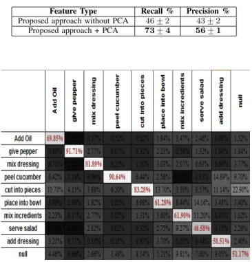
Finally, for internal comparison, Table IV shows the accu-racy improvement achieved by applying PCA to the Fisher vectors. The recall and precision proved much higher than not using PCA (by27and13percentage points, respectively). This is in accordance with the results of [15] that had shown that Fisher vectors are highly compressible. In initial experiments, we had also compared this with the popular VLAD and bag-of-words encodings, but we had achieved much lower accuracies, both with and without PCA.
TABLE IV
RECALL AND PRECISION FOR THE PROPOSED METHOD WITH AND WITHOUTPCA.
Feature Type Recall % Precision % Proposed approach without PCA 46 +−2 43 +−2
Proposed approach + PCA 73+−4 56+−1
Fig. 4. Confusion matrix for the proposed method. Rows and columns represent ground-truth and predicted class labels, respectively. Numbers represent frequencies in percentages and the cells’ gray-levels visually encode the frequencies from 0% = black to 100% = white.
V. CONCLUSION
In this paper, we have proposed a novel approach for fine-grained activity recognition from depth video. The
recognition pipeline includes a novel feature (LDPT), Fisher vector encoding and a contemporary SVM classifier. The experimental results over a probing dataset of kitchen activities have shown that the proposed approach is capable of providing accuracy comparable to that of a state-of-the-art approach that uses a combination of depth/RGB video and accelerometers. We believe that these results pave the way for less intrusive and more pervasive implementations of fine-grained activity monitoring. In addition, the sample frames displayed in Fig. 1 give visual evidence that depth data are very privacy-preserving and can mollify concerns in relation to the adoption of fine-grained activity classification in a variety of environments, including privacy-sensitive organizations such as hospitals and aged care facilities.
REFERENCES
[1] C. Sun, S. Shetty, R. Sukthankar, and R. Nevatia, “Temporal localization of fine-grained actions in videos by domain transfer from web images,” inProceedings of the 23rd ACM International Conference on Multime-dia. ACM, 2015, pp. 371–380.
[2] B. Yao, A. Khosla, and L. Fei-Fei, “Combining randomization and discrimination for fine-grained image categorization,” inProc. CVPR. IEEE, 2011, pp. 1577–1584.
[3] D. Riboni, C. Bettini, G. Civitarese, Z. H. Janjua, and V. Bulgari, “From lab to life: Fine-grained behavior monitoring in the elderlys home,” in
Proc. of PerCom Workshops. IEEE Comp. Soc., 2015.
[4] S. Stein and S. J. McKenna, “Combining embedded accelerometers with computer vision for recognizing food preparation activities,” in
Proceedings of the ACM International Joint Conference on Pervasive and Ubiquitous Computing. ACM, 2013, pp. 729–738.
[5] J. Lei, X. Ren, and D. Fox, “Fine-grained kitchen activity recognition using RGB-D,” inProceedings of the ACM Conference on Ubiquitous Computing. ACM, 2012, pp. 208–211.
[6] M. Rohrbach, S. Amin, M. Andriluka, and B. Schiele, “A database for fine grained activity detection of cooking activities,” inProc. CVPR. IEEE, 2012, pp. 1194–1201.
[7] Y. Zhou, B. Ni, S. Yan, P. Moulin, and Q. Tian, “Pipelining localized semantic features for fine-grained action recognition,” inProc. ECCV. Springer, 2014, pp. 481–496.
[8] M. Stikic, T. Huynh, K. V. Laerhoven, and B. Schiele, “ADL recog-nition based on the combination of RFID and accelerometer sensing,” in Proceedings of the Second International Conference on Pervasive Computing Technologies for Healthcare. IEEE, 2008, pp. 258–263. [9] Y. Chai, V. Lempitsky, and A. Zisserman, “Symbiotic segmentation and
part localization for fine-grained categorization,” inProc. ICCV. IEEE, 2013, pp. 321–328.
[10] J. Donahue, Y. Jia, O. Vinyals, J. Hoffman, N. Zhang, E. Tzeng, and T. Darrell, “DeCAF: A deep convolutional activation feature for generic visual recognition.” inProc. ICML, 2014, pp. 647–655.
[11] Y. Jia, O. Vinyals, and T. Darrell, “Pooling-invariant image feature learning,”arXiv preprint arXiv:1302.5056, 2013.
[12] C. Wah, S. Branson, P. Perona, and S. Belongie, “Multiclass recognition and part localization with humans in the loop,” inProc. ICCV. IEEE, 2011, pp. 2524–2531.
[13] S. Branson, C. Wah, F. Schroff, B. Babenko, P. Welinder, P. Perona, and S. Belongie, “Visual recognition with humans in the loop,” inProc. ECCV. Springer, 2010, pp. 438–451.
[14] L. Xie, Q. Tian, R. Hong, S. Yan, and B. Zhang, “Hierarchical part matching for fine-grained visual categorization,” inProc. ICCV. IEEE, 2013, pp. 1641–1648.
[15] J. S´anchez, F. Perronnin, and Z. Akata, “Fisher vectors for fine-grained visual categorization,” in FGVC Workshop in IEEE Computer Vision and Pattern Recognition (CVPR), 2011.
[16] H. Wang, M. M. Ullah, A. Klaser, I. Laptev, and C. Schmid, “Evaluation of local spatio-temporal features for action recognition,” inProc. BMVC - British Machine Vision Conference. BMVA Press, 2009, pp. 124–1. [17] D. G. Lowe, “Distinctive image features from scale-invariant keypoints,”
International Journal of Computer Vision, vol. 60, no. 2, pp. 91–110, 2004.
[18] H. Bay, A. Ess, T. Tuytelaars, and L. Van Gool, “Speeded-up robust features (SURF),”Computer Vision and Image Understanding, vol. 110, no. 3, pp. 346–359, 2008.
[19] M. Pietik¨ainen, A. Hadid, G. Zhao, and T. Ahonen, “Local binary patterns for still images,” in Computer Vision Using Local Binary Patterns. Springer, 2011, pp. 13–47.
[20] O. Oreifej and L. Zicheng, “HON4D: Histogram of oriented 4d normals for activity recognition from depth sequences,” inProc. CVPR, 2013, pp. 716–723.
[21] L. Xia and J. Aggarwal, “Spatio-temporal depth cuboid similarity feature for activity recognition using depth camera,” inProc. CVPR, 2013, pp. 2834–2841.
[22] Y. Zhao, Z. Liu, L. Yang, and H. Cheng, “Combining RGB and depth map features for human activity recognition,” inProceedings of the Signal & Information Processing Association Annual Summit and Conference (APSIPA ASC), Asia-Pacific. IEEE, 2012, pp. 1–4. [23] M. Pietik¨ainen, G. Zhao, A. Hadid, and T. Ahonen,Computer Vision
Using Local Binary Patterns. Springer, 2011, no. 40.
[24] S. Awwad, F. Hussein, and M. Piccardi, “Local depth patterns for tracking in depth videos,” inProceedings of the 23rd ACM International Conference on Multimedia. ACM, 2015, pp. 1115–1118.
[25] F.-F. Li and P. Perona, “A Bayesian hierarchical model for learning natural scene categories,” in Proc. CVPR. IEEE Computer Society, 2005, pp. 524–531.
[26] H. Jegou, M. Douze, C. Schmid, and P. P´erez, “Aggregating local descriptors into a compact image representation,” inProc. CVPR, 2010, pp. 3304–3311.
[27] F. Perronnin, J. S´anchez, and T. Mensink, “Improving the fisher kernel for large-scale image classification,” inProc. ECCV. Springer-Verlag, 2010, pp. 143–156.
[28] C.-W. Hsu and C.-J. Lin, “A comparison of methods for multiclass support vector machines,”IEEE Trans. Neur. Netw., vol. 13, no. 2, pp. 415–425, Mar. 2002.
[29] Y. Lee, Y. Lin, and G. Wahba, “Multicategory support vector machines: Theory and application to the classification of microarray data and satellite radiance data,”Journal of the American Statistical Association, vol. 99, pp. 67–81, 2004.
[30] Y. Guermeur and E. Monfrini, “A quadratic loss multi-class SVM for which a radius-margin bound applies,” Informatica, Lith. Acad. Sci., vol. 22, no. 1, pp. 73–96, 2011.
[31] F. Lauer and Y. Guermeur, “MSVMpack: A multi-class support vector machine package,”J. Mach. Learn. Res., vol. 12, pp. 2293–2296, Jul. 2011.
[32] C.-C. Chang and C.-J. Lin, “LIBSVM: A library for support vector machines,”ACM Transactions on Intelligent Systems and Technology, vol. 2, pp. 27:1–27:27, 2011.