A Projection-Free Algorithm for Solving Support Vector Machine Models

Clemson University

Clemson University

TigerPrints

TigerPrints

All Theses

Theses

May 2020

A Projection-Free Algorithm for Solving Support Vector Machine

A Projection-Free Algorithm for Solving Support Vector Machine

Models

Models

Seyed Hamid Nazari

Clemson University, [email protected]

Follow this and additional works at: https://tigerprints.clemson.edu/all_theses

Recommended Citation

Recommended Citation

Nazari, Seyed Hamid, "A Projection-Free Algorithm for Solving Support Vector Machine Models" (2020). All Theses. 3361.

https://tigerprints.clemson.edu/all_theses/3361

This Thesis is brought to you for free and open access by the Theses at TigerPrints. It has been accepted for inclusion in All Theses by an authorized administrator of TigerPrints. For more information, please contact

A projection-free algorithm for solving support vector

machine models

A Thesis Presented to the Graduate School of

Clemson University

In Partial Fulfillment of the Requirements for the Degree

Master of Science Mathematics by HamidNazari May 2020 Accepted by:

Dr. Yuyuan Ouyang, Committee Chair Dr. Cristopher McMahan

Abstract

In this thesis our goal is to solve the dual problem of the support vector machine (SVM) problem, which is an example of convex smooth optimization problem over a polytope. To this goal, we apply the conditional gradient (CG) method by providing explicit solution to the linear programming (LP) subproblem. We also describe the conditional gradient sliding (CGS) method that can be considered as an improvement of CG in terms of number of gradient evaluations. Even though CGS performs better than CG in terms of optimal complexity bounds, it is not a practical method because it requires the knowledge of the Lipschitz constant and also the number of iterations. As an improvement of CGS, we designed a new method,conditional gradient sliding with line search (CGS-ls) that resolves the issues in CGS method. CGS-ls requires O(1/√) gradient evaluations andO(1/) linear optimization calls that achieves the optimal complexity bounds in CGS method. We also compare the performance of our method with CG and CGS methods as numerical results by experimenting them in dual problem of SVM for binary classification of two subsets of the MNIST hand-written digits dataset.

Table of Contents

1.1 Properties of convex smooth functions . . . 2

1.2 Support Vector Machine . . . 4

1.3 Projection-based Algorithms . . . 7

1.4 Examples of projections . . . 14

1.5 Projection-free Algorithms . . . 20

2 CGS With Line Search . . . 46

3 Experimental results . . . 59

3.1 Binary classification of 2D data set . . . 60

3.2 Binary classification of MNIST hand-written digits . . . 64

List of Tables

List of Figures

3.1 Classifying 2D data sets in two orthants . . . 61

3.2 accuracy of algorithms classifying data sets in two orthants . . . 61

3.3 iteration versus objective value in classifying data sets in two orthants . . . 61

3.4 CPU-time versus objective value in classifying data sets in two orthants . . . 61

3.5 CPU-time versus accuracy in classifying data sets in two orthants . . . 62

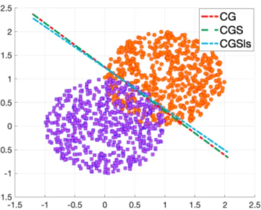
3.6 Classifying 2D data sets . . . 63

3.7 accuracy of algorithms . . . 63

3.8 iteration versus objective value in classifying data sets in two unit balls . . . 63

3.9 CPU-time versus objective value in classifying data sets in two unit balls . . . 63

3.10 CPU-time versus accuracy in classifying data sets in two unit balls . . . 63

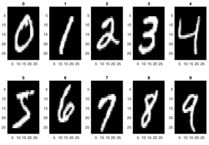
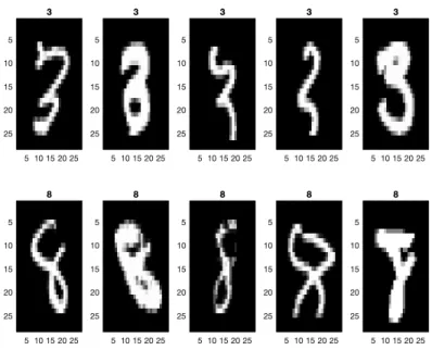
3.11 a sample of converted MNIST data set to images. . . 64

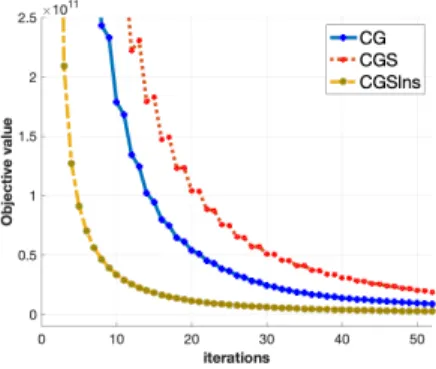
3.12 Iterations versus objective value. . . 65

3.13 CPU time versus Objective value. . . 65

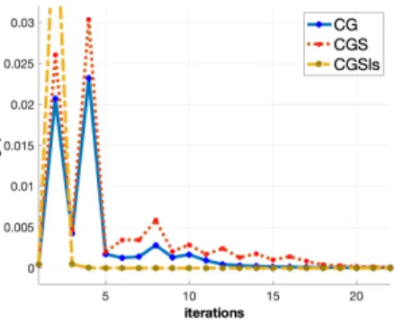
3.14 Iterations versus Wolfe gap. . . 66

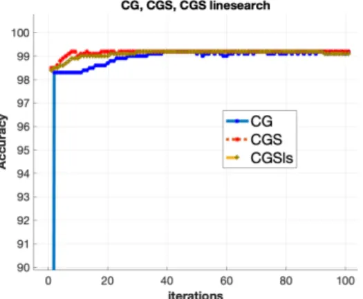
3.15 Iterations versus accuracy. . . 66

3.16 CPU-time versus Wolfe gap. . . 66

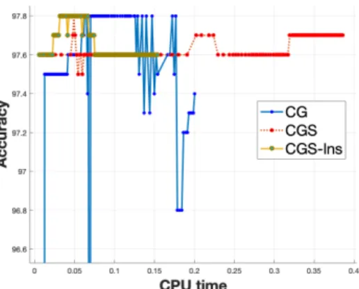
3.17 CPU-time versus accuracy. . . 66

Chapter 1

Introduction

In this thesis our problem of interest is

min

x∈X f(x) (1.1)

whereX ⊆Rnis a convex compact set andf :Rn→Ris a smooth convex function. We assume that

the gradient function ∇f(·) is Lipschitz continuous (with respect to the normk·k) with Lipschitz constantL >0, namely

k∇f(x)− ∇f(y)k_∗≤Lkx−yk, ∀x, y∈_Rn_{. (1.2)}

Herek·kis any norm and k·k_∗ is its dual norm, defined by

kyk_∗:= sup

kxk≤1

hx, yi

fory∈Rn. Also, we define the diameter of the setX as

DX ≡DX,k·k:= max

x,y∈Xkx−yk. (1.3)

Throughout this chapter, we describe the properties and examples of problem (1.1), and also list several algorithms that can solve (1.1).

1.1

Properties of convex smooth functions

In this section we describe a few properties of convex smooth functions. These properties are necessary for analyzing the algorithms that we are going to introduce in the sequel. We start with the definition of a convex function.

Definition 1. A function f :Rn→Ris a convex function if for anyx, y∈Rn and any λ∈[0,1],

we have

f(λx+ (1−λ)y)≤λf(x) + (1−λ)y. (1.4)

We say thatf is concave if (−f) is convex. An important property of convex functions can be shown by an induction through our definition in (1.4):

f k X i=1 λixi ! ≤ k X i=1 λif(xi), (1.5)

for allλ1, . . . , λk ∈[0,1] such thatP k

i=1λi= 1 and allxi∈Rn, i= 1,· · ·, k. In such case,Pki=1λixi is called a convex combination ofx1, . . . , xk. We are now ready to introduce two important properties of convex smooth functions.

Proposition 1. Let f :Rn→Rbe a smooth function that satisfies (1.2), then

|f(y)−f(x)− h∇f(x), y−xi | ≤ L

2 ky−xk

2

, ∀x, y∈Rn. (1.6)

Proof. Let us fix anyx, y∈Rn and define

h(τ) :=f((1−τ)x+τ y), ∀τ ∈[0,1].

Then we haveh(0) =f(x),h(1) =f(y), and

By the fundamental theorem of calculus, we have h(1) =h(0) + Z 1 0 h0(τ)dτ, i.e., f(y) =f(x) + Z 1 0 h∇f((1−τ)x+τ y), y−xidτ =f(x) +h∇f(x), y−xi+ Z 1 0 h∇f((1−τ)x+τ y)−f(x), y−xidτ. Therefore |f(y)−f(x)− h∇f(x), y−xi|= Z 1 0 h∇f((1−τ)x+τ y)−f(x), y−xidτ ≤ Z 1 0 |h∇f((1−τ)x+τ y)−f(x), y−xi| dτ ≤ Z 1 0 k∇f((1−τ)x+τ y)−f(x)k_∗ky−xk dτ ≤ Z 1 0 Lτky−xk2 dτ = L 2 ky−xk 2 .

Here in the second inequality we use the Cauchy-Schwartz inequality.

Theorem 1. A smooth functionf :Rn→R is convex if and only if

f(y)≥f(x) +h∇f(x), y−xi, ∀x, y∈Rn. (1.7)

Proof. Let us fix anyx, y∈_Rn_{, and denote x}

λ:=λx+ (1−λ)y. Suppose that (1.7) holds. Then for anyλ∈[0,1] we have

f(x)≥f(xλ) +h∇f(xλ), x−xλiandf(y)≥f(xλ) +h∇f(xλ), y−xλi.

Noting thatx−xλ= (1−λ)(x−y) andy−xλ=λ(y−x), using the above relations, we have

=f(xλ), ∀λ∈[0,1].

Therefore (1.4) holds andf is convex. Let us consider the other direction and suppose that (1.4) holds. Then for anyλ∈[0,1) we have

f(xλ)≤λf(x) + (1−λ)f(y), or f(y)≥ f(xλ)−λf(x) 1−λ =f(x) + f(xλ)−f(x) 1−λ . (1.8) Lettingλ→1, we have lim λ→1 f(xλ)−f(x) 1−λ =−λlim→1 f(y+λ(x−y))−f(x) λ−1 =− d dλ _λ=1f(y+λ(x−y)) =−hf(x), x−yi. (1.9)

Combining (1.9) and (1.8) we obtain (1.7) and conclude the theorem.

From Proposition 1 and Theorem 1, we can prove the following corollary immediately.

Corollary 1. Letf be a convex smooth function. We have,

0≤f(y)−f(x)− h∇f(x), y−xi ≤L

2ky−xk

2_{, ∀x, y∈}

Rn. (1.10)

1.2

Support Vector Machine

In this section, we describe an example of (1.1). Suppose that we have a set of points in

Rn and we would like to classify these points intok sets. This problem is called classification in

machine learning. One classification model is the support vector machine (SVM). There are two types of SVMs, namely hard-margin SVM and soft-margin SVM. In this section, we describe the soft-margin SVM.

Suppose that we havek= 2 sets of data points. LetX∈Rn×mbe the matrix corresponding

binary classification, namely, we are distinguishing two classes of data points. The optimization problem of the soft-margin SVM model [4] can be expressed as

min w∈Rm,ξ∈Rn,w0∈R 1 2kwk 2 2+C n X i=1 ξi s.t. bi(hw, Xii −w0)≥1−ξi, i= 1, . . . , n ξi≥0. (1.11)

Here ξ := (ξ1,· · ·, ξn)T and XiT denotes the ith row of X. We will formulate the dual problem of (1.11). The Lagrangian function corresponding to (1.11) is

L(w, w0, ξ, x, λ) = 1 2kwk 2_+C n X i=1 ξi− n X i=1 xi bi(wTXi+w0)−1 +ξi − n X i=1 λiξi = 1 2w T_w+C n X i=1 ξi− n X i=1 xibiwTXi− n X i=1 xibiw0+ n X i=1 xi− n X i=1 xiξi− n X i=1 λiξi = 1 2w T_w−wT n X i=1 xibiXi− n X i=1 xibiw0+ (C−xi−λi) n X i=1 ξi+ n X i=1 xi

wherex= (x1,· · · , xn)T andλ= (λ1,· · ·, λn)T. So the Lagrangian dual will be

zD= sup λ≥0,x≥0 inf w∈Rn,ξ∈Rm,w0∈R L(w, w0, λ) or zD= sup λ≥0,x≥0 n X i=1 xi+ inf w∈Rm,ξ∈Rn,w0∈R 1 2w T_w−wT n X i=1 xibiXi− n X i=1 xibiw0+ (C−xi−λi) n X i=1 ξi !!

Calling the function inside the inf function ash(w, ξ, w0) wherew, ξ∈Rn andw0∈R, we

can observe that the functionhis convex with respect towand is affine with respect to ξandw0.

infw,w0h(w, w0). So forwwe have: ∇wh(w, ξ, w0) = w− n X i=1 xibiXi= 0 ⇒ w∗= n X i=1 xibiXi (1.12) ∇ξh(w, ξ, w0) = C−xi−λi = 0, i= 1,· · ·, n (1.13) ∇w0h(w, ξ, w0) = n X i=1 xibi= 0. (1.14)

Having foundw∗ we can findw∗₀. Since we require the interceptw₀∗ to satisfy

w∗0≤ −1− max i:bi=−1 w∗TXi (1.15) w∗₀≥ 1− min i:bi=1 w∗TXi, (1.16)

we takew∗₀ to be the average the two values (1.15) and (1.16). Hence,

w∗₀=−maxi:bi=−1w ∗T_X i+ mini:bi=1w ∗T_X i 2 . (1.17)

Also, for anywandw0we have ξi = 1−bi(hw, Xii −w0), i= 1,· · · , n. Therefore,

ξ∗i = 1−bi(hw∗, Xii −w∗0), i= 1,· · ·, n. (1.18)

Substituting the optimal solutionw∗, w∗₀ andξ∗to infw,w0h(w, ξ, w0) we obtain:

inf w∈Rm,ξ∈Rn,w0∈R h(w, ξ, w0) = 1 2   m X j=1 xjbjXj   n X i=1 xibiXi ! −   m X j=1 xjbjXj   n X i=1 xibiXi ! =−1 2   m X j=1 xjbjXj   n X i=1 xibiXi ! =−1 2 m X j=1 n X i=1 xixjbibjXiTXj =−1 2 m X j=1 n X i=1 xixjbibjhXi, Xji.

Note that we must havexi, λi ≥0. Also, from (1.13) we have λi =C−xi. Therefore, we must havexi≤C. Summarizing the above derivation, the Lagrangian dual of (1.11) can be written as

sup x∈Rn n X i=1 xi− 1 2 m X j=1 n X i=1 xixjbibjhXi, Xji s.t. n X i=1 xibi = 0 0≤xi≤C i= 1, . . . , n. (1.19)

Note that the above is a special case of (1.1) with convex quadratic objective function

f(x) := n X i=1 xi− 1 2 m X j=1 n X i=1 xixjbibjhXi, Xji

and polytope feasible set

X := ( x : n X i=1 xibi= 0, 0≤xi≤C, i= 1, . . . , n ) .

Now we are ready to introduce and analyze some types of algorithms to solve (1.1). In general, we will discuss two types of algorithms, projection-based algorithms and projection-free algorithms. At each part, we will discuss the advantages and also the drawbacks of each type of algorithm.

1.3

Projection-based Algorithms

Projection-based algorithms are of the type that need projection as their subproblems. The projections that appear in these algorithms might be different depending on the problem structure. In this section we will describe and analyze theprojected gradientandNesterov’s accelerated gradient descent methods [10]. After analyzing these algorithms we will have a section to provide several examples of projection to different sets that might appear in these algorithms as a subproblem.

1.3.1

Projected gradient method

As we can see from the name of this algorithm, projected gradient method is a projection-based algorithm. Projected gradient is one of the most straight forward projection-projection-based algorithms. The simplest interpretation of this algorithm is that at each step we go through the negative direction

of the objective; if we are out side of the feasible set then we project back the point to the feasible set and continue with the projected point. We will describe a more general form of the projected gradient method usingprox-function.

The algorithm of projected gradient method for solving (1.1) is described bellow.

Algorithm 1 The gradient descent algorithm Choosex0∈ X. fork= 1, . . . , N do xk= arg min x∈X h∇f(xk−1), xi+ηkV(xk−1, x) (1.20) end for OutputxN.

HereV(·,·) is a function, called theprox function, that satisfies the following two inequalities: 1. For anyx, y∈Rn,

V(x, y)≥ 1

2kx−yk

2_{. (1.21)}

2. For anyg∈Rn andu∈Rn, ify is the solution to the problem

min

x∈Xhg, xi+ηV(u, x), then

hg, y−xi ≤η[V(u, x)−V(u, y)−V(y, x)], ∀x∈ X. (1.22)

The simplest choice of V(·,·) is V(x, y) := ky−xk2

2/2, when the norms k · k and k · k∗ are both

2-norms. Note also that the gradient method is a special case of Algorithm 2 withγk ≡1,X =Rn,

V(x, y) := ky −xk2

V(xk−1, x) =kx−xk−1k 2

2/2, then (1.20) in Algorithm 1 becomes

xk = arg min x∈Rn h∇f(xk−1), xi+ ηk 2 kx−xk−1k 2 2 = arg min x∈Rn ηk 2 x−xk−1+ 1 ηk ∇f(xk−1) 2 =xk−1− 1 ηk ∇f(xk−1). (1.23)

The geometric interpretation of above is clear; the new iterationxk is computed by moving from xk−1 along the opposite direction of∇f(xk−1) with stepsize 1/ηk. The intuition is that the negative direction−∇f(x) is the direction of the fastest local decrement off at point x.

In the following theorem, we state the convergence result of the projected gradient algorithm in Algorithm 1, assuming constant stepsize.

Theorem 2. Suppose that f : _Rn _→

R is a smooth convex function. If the parameters ηk in Algorithm 1 satisfy ηk≡η≥L, (1.24) then we have f(¯xN)−f∗≤ η NV(x0, x ∗_), where ¯ xN := 1 N N X k=1 xk.

Proof. Sincef is a smooth convex function, from the Corollary 1 and Theorem 1 we have

f(xk)≤f(xk−1) +h∇f(xk−1), xk−xk−1i+ L 2kxk−xk−1k 2 2 =f(xk−1) +h∇f(xk−1), x−xk−1i+h∇f(xk−1), xk−xi+ L 2 kxk−xk−1k 2 (1.25) ≤f(x) +h∇f(xk−1), xk−xi+ η 2kxk−xk−1k 2 (1.26) ≤f(x) +η(V(xk−1, x)−V(xk−1, xk)−V(xk, x)) +ηV(xk, xk−1) (1.27)

=f(x) +η(V(xk−1, x)−V(xk, x)),

where the equality (1.25) is from (1.24), inequality (1.26) is from convexity of f, and inequality (1.27) is from (1.22). Hence,

f(xk)≤f(x) +η(V(xk−1, x)−V(xk, x)).

Summing the above inequality up fromk= 1 toN, we obtain N

X

k=1

f(xk)≤N f(x) +η(V(xk−1, x)−V(xk, x))

≤N f(x) +ηV(x0, x).

Settingx=x∗ in above relation and using the convexity off, we have

f(¯xN)≤ 1 N N X k=1 f(xk)≤f(x∗) + η NV(x0, x ∗_). Therefore, f(¯xN)−f∗≤ η NV(x0, x ∗_).

From the above theorem, we observe that in order to compute an approximate solution ¯xN such thatf(¯xN)−f∗≤ε, the number of iterations that are required is bounded byO(LV(x0,x∗)/).

1.3.2

Nesterov’s accelerated gradient method

In the previous section we obtained anO(1_{/) convergence result of the projected gradient}

descent method. In this section we introduce a method that has a better complexity. This algo-rithm is called Nesterov’saccelerated gradient descent(AGD) method. Similar to projected gradient descent, AGD is a projection-based algorithm.

The algorithm of accelerated gradient descent method for solving (1.1) is described bellow.

Algorithm 2Accelerated Gradient Descent Method Choosex0∈ X and set y0=x0.

fork= 1,· · · , N do zk = (1−γk)yk−1+γkxk−1 (1.28) xk = arg min x∈X h∇f(zk), xi+ηkV(xk−1, x) (1.29) yk = (1−γk)yk−1+γkxk (1.30) end for OutputyN.

We present the convergence result of Algorithm 2. In Theorem 3 below we describe a general result.

Theorem 3. Suppose thatyk andzk in Algorithm 2 satisfy

f(yk)≤f(zk) +h∇f(zk), yk−zki+

Lk

2 kyk−zkk

2 _(1.31)

for someLk >0, and that the parameters in Algorithm 2 satisfy

γ1= 1, γk ∈[0,1), andηk≥Lkγk, ∀k≥1. (1.32)

Letting Γk be a parameter that satisfiesΓ1>0 and

Γk= (1−γk)Γk−1, ∀k >1, (1.33) then we have f(yk)−f∗≤Γk k X i=1 γiηi Γi [V(xi−1, x∗)−V(xi, x∗)], wherex∗ is a solution to (1.1).

Proof. Noting (1.28) and (1.30) we haveyk−zk =γk(xk−xk−1), and also yk−zk =yk−yk−1+yk−1−zk (1.30) = γk(xk−yk−1) +yk−1−zk =γk[(xk−x) + (x−zk) + (zk−yk−1)] +yk−1−zk = (1−γk)(yk−1−zk) +γk((x−zk) + (xk−x)) = (1−γk)(yk−1−zk) +γk(xk−zk). (1.34)

Using above the inequality, (1.31) becomes

f(yk)≤f(zk) + (1−γk)h∇f(zk), yk−1−zki+γkh∇f(zk), xk−zki+ Lkγk2 2 kxk−xk−1k 2 = (1−γk)[f(zk) +h∇f(zk), yk−1−zki] +γk[f(zk) +h∇f(zk), x−zki+h∇f(zk), xk−xi] +Lkγ 2 k 2 kxk−xk−1k 2_{, ∀x∈ X.}

Let us make three observations. First, by (1.10), we have

f(zk) +h∇f(zk), yk−1−zki ≤f(yk−1),

and

f(zk) +h∇f(zk), x−zki ≤f(x).

Second, by (1.22) (withg=∇f(zk),y=xk, u=xk−1, andη =ηk) we have

h∇f(zk), xk−xi ≤ηk[V(xk−1, x)−V(xk−1, xk)−V(xk, x)], ∀x∈ X. Third, by (1.21), we have Lkγk2 2 kxk−xk−1k 2 ≤Lkγk2V(xk−1, xk).

Summarizing the three observations, we have f(yk)≤(1−γk)f(yk−1) +γkf(x) +γkηk[V(xk−1, x)−V(xk−1, xk)−V(xk, x)] +Lkγk2V(xk−1, xk) = (1−γk)f(yk−1) +γkf(x) +γkηk[V(xk−1, x)−V(xk, x)] −γk(ηk−Lkγk)V(xk−1, xk) ≤(1−γk)f(yk−1) +γkf(x) +γkηk[V(xk−1, x)−V(xk, x)].

Here the last inequality is from (1.32). Summing up the above two inequalities, we have

f(yk)≤(1−γk)f(yk−1) +γkf(x) +γkηk[V(xk−1, x)−V(xk, x)].

In particular, lettingx=x∗ wherex∗ is a solution to (1.1), we can reformulate the above to

f(yk)−f∗≤(1−γk)(f(yk−1)−f∗) +γkηk[V(xk−1, x∗)−V(xk, x∗)].

Dividing both sides by Γk, and using (1.33) and (1.32), we have

1 Γk (f(yk)−f∗)≤ 1 Γk−1 (f(yk−1)−f∗) + γkηk Γk [V(xk−1, x∗)−V(xk, x∗)], ∀k >1.

Also, whenk= 1, noting that γ1= 1 by (1.32), we have

1 Γ1 (f(yk)−f∗)≤ γ1η1 Γ1 [V(x0, x∗)−V(x1, x∗)].

Using induction on the two inequalities above, we conclude that

1 Γk (f(yk)−f∗)≤ k X i=1 γiηi Γi [V(xi−1, x∗)−V(xi, x∗)].

Corollary 2. If we set γk= 2 k+ 1, ηk= 2L k (1.35) in Algorithm 2, then f(yk)−f∗≤ 4L k(k+ 1)V(x0, x ∗_{). (1.36)}

Proof. Clearly (1.31) and (1.32) hold, and Γk =2/k(k+1)satisfies (1.33) with Γ1= 1. Therefore, by

Theorem 3, we have f(yk)−f∗≤ 2 k(k+ 1) k X i=1 2L[V(xi−1, x∗)−V(xi, x∗)] = 4L k(k+ 1)[V(x0, x ∗_)−V(x k, x∗)]. (1.37)

From (1.21), we haveV(xk, x∗)≥0. Thus

f(yk)−f∗≤ 4L

k(k+ 1)V(x0, x

∗_{). (1.38)}

From Corollary 2 we can see that in order to compute an approximate solution such that

f(yk)−f∗≤ε, we need

k≥

r

4LV(x0, x∗)

ε . (1.39)

Therefore, the iteration complexity upper bound is O(p1_{/ε). Note that the Nesterov’s accelerated}

gradient method is optimal for solving smooth convex optimization with Lipschitz constantL[10].

1.4

Examples of projections

In this section we have some examples of projections of different sets. As we have seen in previous sections these projections arise from the subproblems of the projection-based algorithms.

1.4.1

Projection onto the standard simplex under the Euclidean

prox-function

Assume thatX in (1.1) is a standard simplex ∆n. We will study the projection subproblem (1.29) in Algorithm 2 where the prox-function is defined as

V(x, y) = 1

2kx−pk

2

, p∈Rn.

Note that similar analysis can be performed for Algorithm 1. The subproblem (1.29) in this case can be formulates as

min x∈Rn h∇f(zk), xi+ ηk 2 kx−pk 2 (1.40) s.t. −x(i)≤0 i= 1,· · · , n (1.41) n X i=1 x(i)−1 = 0 (1.42)

and without loss of generality we can assume thatp∈Rn satisfiesp(1)≤p(2)≤ · · · ≤p(n).

To solve the problem (1.4.1) since the Slater’s condition holds we may consider the KKT points a) Primal feasibility −x(i)≤0 i= 1,· · ·, n n X i=1 x(i)−1 = 0 b) Complementary slackness −u(i)x(i)= 0, ∀i= 1,· · ·, n c) Dual feasiblity ∇f(zk)(i)+x(i)−p(i)−u(i)+v= 0, ∀i= 1,· · ·, n u(i)≥0, ∀i= 1,· · ·, n

For anyi= 1,· · · , nifu(i)= 0, then by dual feasibility we have

x(i)=p(i)−v− ∇f(zk)(i).

Sincex(i)_{≥0, we needp}(i)_≥v+∇f(z

k)(i).Ifu(i)>0, then from complementary slackness we have

x(i)_{= 0 and by dual feasibility}

u(i)=v−p(i)+∇f(zk)(i)

and sinceu(i)>0, thenp(i)< v+∇f(zk)(i). In summary,

x(i)=      p(i)_{−v− ∇f(z} k)(i) ifp(i)≥v+∇f(zk)(i) 0 otherwise.

Note that from primal feasibility and dual feasibility we have

1−

n

X

i=1

(p(i)+u(i)− ∇f(zk)(i)) +nv= 0,

which implies that

v= 1 n n X i=1 (p(i)+u(i)− ∇f(zk)(i)) ! − 1 n = 1 n   X i:p(i)_≥v+∇f(z k)(i) (p(i)− ∇f(zk)(i)) + X i:p(i)_<v+∇f(z k)(i) v  − 1 n or X i:p(i)_{≥v+∇f(zk)}(i) v= X i:p(i)_{≥v+∇f(zk)}(i) (p(i)− ∇f(zk)(i))−1.

Therefore, we have the following cases: i) v≤p(1)_{− ∇f(z} k)(1). In this case nv= n X i=1 (p(i)− ∇f(zk)(i))−1 or v= 1 n n X i=1 (p(i)− ∇f(zk)(i))− 1 n

ii) p(j)− ∇f(zk)(j)< v≤p(j+1)− ∇f(zk)(j+1). In this case (n+j)v= n X i=j+1 (p(i)− ∇f(zk)(i))−1 iii) v > p(n)_{− ∇f(z} k)(n)which is infeasible. Hence, we havenpossible choices ofvas

v=      1 n Pn i=1(p (i)_{− ∇f(z} k)(i))−_n1 ifnp(1)≥P n i=1(p (i)_{− ∇f(z} k)(i))−1 1 n+j Pn i=j+1(p (i)_{− ∇f(z} k)(i))−_n+1_j if (n+j)p(j)≥P n i=1(p (i)_{− ∇f(z} k)(i))−1≤(n+j)p(j+1) wherej= 1,· · · , n−1. The optimal solution is of the form

(x∗)(i)=      p(i)−v− ∇f(zk)(i) ifp(i)≥v+∇f(zk)(i) 0 otherwise.

1.4.2

Projection onto the standard simplex under entropy prox-function

If we define the prox-function in (1.29) as

V(x, y) =ω(x)−ω(y)− h∇ω(y), x−yi, (1.43)

whereω(x) =Pn

i=1x

(i)_logx(i)_{, then we have}

arg min x∈∆n h∇f(zk), xi+ηk(ω(x)−ω(xk−1)− h∇ω(xk−1), x−xk−1i) = arg min x∈∆n h∇f(zk), xi +ηk n X i=1 x(i)logx(i)− n X i=1 (xk−1)(i)logx (i) k−1− n X i=1 (logx(_ki₋)₁+ 1)(x(i)−x(_ki₋)₁) ! = arg min x∈∆n h∇f(zk), xi+ηk n X i=1 x(i)log x (i) x(_ki₋)₁ − n X i=1 x(i)+ n X i=1 x(_ki₋)₁ ! = arg min x∈∆n h∇f(zk), xi+ηk n X i=1 x(i)log x (i) x(_ki₋)₁

= arg min x∈∆n h∇f(zk), xi+ηk n X i=1 x(i)logx(i)−ηk n X i=1 x(i)logx(_ki₋)₁ = arg min x∈∆n * 1 ηk ∇f(zk)−       logx(1)_k−1 .. . logx(_kn₋)₁       , x + + n X i=1 x(i)logx(i).

Now we rewrite the subproblem (1.29) as

min x∈Rn h∇f(zk), xi+ηk n X i=1 x(i)log x (i) x(_ki₋)₁ s.t. −x(i)≤0 n X i=1 x(i)−1 = 0 Or equivalently min x∈Rn hg, xi+ n X i=1 x(i)logx(i) s.t. −x(i)≤0 n X i=1 x(i)−1 = 0 (1.44) where g = _η1 k∇f(zk)−       logx(1)_k−1 .. . logx(_kn₋)₁      

. The optimization problem (1.44) is the subproblem of the

accelerated gradient descent method with prox-function defined in (1.43). Proposition 2 gives the solution to the above.

Proposition 2. Let X in subproblem of Algorithm 2 be the standard simplex defined as

∆n ={x∈Rn :

n

X

i=1

x(i)= 1, x(i)≥0, i= 1,· · ·, n}.

and the prox-function V(·,·) be of the form (1.43), where ω(x) :=Pn

i=1x

element of the optimal solutionx∗ to the subproblem (1.44)is (x∗)(i)= e −g(i) Pn i=1e−g (i).

Proof. To solve the problem (1.44) since the Slater’s conditions hold we check the KKT points a) Primal feasibility: n X i=1 x(i)= 1 x(i)≥0 b) Complementary slackness: −u(i)x(i)= 0, ∀i= 1,· · ·, n c) Dual feasibility: g(i)+ logx(i)+ 1−u(i)+v= 0, ∀i= 1,· · ·, n u(i)≥0, ∀i= 1,· · ·, n

Since for any i, x(i) _{>0, then we must have u}(i) _{= 0, ∀i = 1,· · ·, n. This implies that}

logx(i)_=−g(i)_{−1−v and so} x(i)= 1 e1+v_×eg(i). SincePn i=1x(i)= 1 we conclude that 1 = 1 e1+v n X i=1 e−g(i)

Taking log from both sides and writing the equality with respect tov we get

v= log n X i=1 e−g(i) ! −1

Therefore (x∗)(i) = 1 exp logPn i=1e−g (i) eg(i) = e −g(i) Pn i=1e−g (i).

Note that the choice ofV(·,·) in Proposition 2 is also called the entropy prox-function.

1.5

Projection-free Algorithms

In previous section we mentioned projected gradient and accelerated gradient descent as ex-amples of projection-based methods. These methods require projection as subproblems and specially the AGD with complexityO(p1_{/) is an efficient algorithm. However, the projection in subproblems}

of these algorithms are sometimes problematic. They are not always efficiently solvable. Algorithms called projection-free algorithms are useful in such expensive cases.

Similar to previous section, we mention some of the projection free algorithms and discuss their complexities. The methods that we are going describe areconditional gradientandconditional gradient sliding. We will compare their complexity with themselves and also with projection-based algorithm that we had in the last section.

1.5.1

Conditional Gradient Algorithm

Conditional gradient (CG) algorithm, also known as Frank-Wolfe method, is one of the earliest projection-free first-order algorithms for solving convex programming problems. It was initially developed by Frank and Wolfe in 1956 [5]. The algorithm of CG is described in Algorithm 3.

As we can observe in Algorithm 3, the CG method solves the projection subproblem (1.29) of AG approximately over the feasible setX. Regarding the CG algorithm we should mention a few remarks. First, in CG method the assumption of compactness ofX is important, because otherwise the subproblem (1.46) might become unbounded. Second, the solution to (1.46) is not necessarily unique and there might exist multiple solutions. Third, it is better to avoid settingγk ≡1. As an

example, consider the problem withf(x) =x2and X = [−1,1]. Settingx0=z0= 1 where γk ≡1 imply that the CG method hasx1=x3=· · ·= 1 and x0=x2=· · ·=−1 as its outputs.

Algorithm 3Conditional Gradient Algorithm Choosez0∈ X and setx0=z0.

fork= 1,· · · , N do zk = (1−γk)yk−1+γkxk−1 (1.45) xk ∈ Argmin x∈X h∇f(zk), xi (1.46) yk = (1−γk)yk−1+γkxk (1.47) end for OutputxN.

We describe the convergence result [5] of the CG method in Algorithm 3. We first state a simple technical result that will be used in the analysis of the algorithm.

Lemma 1. Let wt∈(0,1], t= 1,2,· · ·, be given. Also let us denote

Wt:=      1, t= 1, (1−wt)Wt−1, t≥2. (1.48)

Suppose thatWt>0 for allt≥2 and that the sequence{δt}t≥0 satisfies

δt≤(1−wt)δt−1+Bt, t= 1,2,· · ·. (1.49)

Then for any1≤l≤k, we have

δk ≤Wk 1−wl Wl δl−1+ k X i=l Bi Wi ! . (1.50)

Proof. Dividing both sides of (1.49) byWt, we obtain

δ1 W1 ≤ (1−w1)δ0 W1 + B1 W1

and δi Wi ≤(1−wi)δi−1 Wi + Bi Wi = δi−1 Wi−1 + Bi Wi ∀i≥2.

The result then immediately follows by summing up the above inequalities for i = 1· · ·, k and rearranging the terms.

In the following theorem and corollary the notation below will be used:

Γk=      1 ifk= 1 (1−γk)Γk−1 ifk≥2. (1.51)

Theorem 4. For parametersγk∈(0,1) in Algorithm we have

f(yk)−f∗≤ LD2_Γ k 2 k X i=1 γ2 i Γi . (1.52)

Proof. Fist, we can write (1.47) asyk =yk−1+γk(xk−yk−1), so

yk−yk−1=γk(xk−yk−1). (1.53)

Also, from (1.45) and (1.45) we observe that

yk−zk =yk−yk−1+yk−1−zk (1.53) = γk(xk−yk−1) +yk−1−zk =γk[(xk−x) + (x−zk) + (zk−yk−1)] +yk−1−zk =γk((x−zk) + (xk−x)) + (1−γk)(yk−1−zk). (1.54)

Sincef is a smooth convex function from Corollary (1) and also from (1.47) we have

f(yk)≤f(zk) +h∇f(zk), yk−zki+

L

2 kyk−zkk

2

. (1.55)

Now from (1.54), for anyx∈X we have

+γk[f(zk) +h∇f(zk), x−zki+h∇f(zk), xk−xi] +L 2 kyk−zkk 2 = (1−γk)(f(zk) +h∇f(zk), yk−1−zki) +γk(f(zk) +h∇f(zk), x−zki) +γkh∇f(zk), xk−xi+ L 2 kyk−zkk 2 .

Here we note that since xk is an optimal solution to the subproblem (1.46), then by optimality condition we have

h∇f(zk), xk−xi ≤0,

and also sincef is a convex function we have

f(zk) +h∇f(zk), yk−1−zki ≤f(yk−1)

and

f(zk) +h∇f(zk), x−zki ≤f(x).

In addition, from (1.45) and (1.47) we haveyk−zk=γk(xk−xk−1). Summarizing all these

and using (1.3) we obtain

f(yk)≤(1−γk)f(yk−1) +γkf(x) + Lγ2 k 2 D 2_, or equivalently, f(yk)−f(x)≤(1−γk)(f(yk−1)−f(x)) + Lγ_k2 2 D 2_.

Dividing both sides of the above inequality by Γk fork≥2 we obtain

f(yk)−f(x) Γk ≤ (1−γk) Γk (f(yk−1)−f(x)) + Lγ2 k 2Γk D2.

Also, fork= 1 we have

f(y1)−f(x)≤

LD2_γ2 1

2 .

Summing up from 1 tokwe conclude that

1 Γk (f(yk)−f(x))≤ LD2 2 k X i=1 γ2 i Γi .

Note that the sequence of parameters γk in CG is conceptual and clearly there might be many choices to set these parameters properly to get the best convergence result for this algo-rithm. In Corollary 3 below we provide a setting for this parameter and prove the convergence rate corresponding to our setting.

Corollary 3. In Algorithm 3, if we set the parameterγk=2/(k+1), then

f(yk)−f∗≤ 2LD2

k+ 1. (1.56)

Proof. Withγk defined in assumption we have

Γk = 2 k(k+ 1). (1.57) Using (1.57) we obtain k X i=1 γ2 i Γi = k X i=1 4 (i+ 1)2 × i(i+ 1) 2 = k X i=1 2i i+ 1 = 2( k X i=1 1− k X i=1 1 i+ 1)≤2k. Therefore, f(yk)−f∗ ≤ LD2 2 × 2 k(k+ 1)×2k = 2LD 2 k+ 1.

Corollary 3 shows that the CG method computes an -solution to the problem (1.1) in

O(LD2_{/) iterations. This means that in order to compute ansolution, CG requires more evaluations} of ∇f than AGD method, which only requiresO(p1_{/) evaluations. This drawback is resolved in} conditional gradient sliding method [8]. In particular, conditional gradient sliding method requires

O(p1_{/) evaluations of∇f(·) andO(}1_{/) evaluations for linear optimization problems of form (1.46).}

we will discuss the conditional gradient sliding method in later sections.

According to [6, 9] the number of evaluations of linear optimization problems of form (1.46) can not be improved from the lower complexity boundO(1_{/). Also, it should be noted that the CG}

does not require knowledge on the Lipschitz constantL, the normk.k, and diameterD. In particular, if there exists a normk.kthat yields the smallest possible value ofLD2, then the convergence result (1.56) will follow such smallest value. In other words, the CG is a first-order method that would automatically adapt to the best possible geometric properties of the problem.

1.5.2

Conditional Gradient Sliding Algorithm

In this section we describe an algorithm and its analysis by [8]. The goal of theconditional gradient sliding(CGS) [8] method is to present a new linear optimization based convex programming method which can skip the computation for the gradient of f from time to time when performing Linear optimization over the feasible region X. The basic scheme of this method is obtained by applying the CG method to solve the projection subproblems existing in the AGD approximately. By properly specifying the accuracy for solving these subproblems, we will show that the resulting CGS method can achieve the optimal bounds on the number of calls to the first-order and linear optimization oracles for solving problem (1.1). The development of CGS method, in spirit, is similar to the gradient sliding algorithm developed by Lan in [7] for solving a class of composite optimization problems. However, the gradient sliding algorithm in [7] requires us to perform projection over the feasible setX and targets to solve convex programming problems with a general nonsmooth term in objective function. The CGS method is formally described in Algorithm 4.

Algorithm 4 The Conditional Gradient Sliding Algorithm Initial pointx0∈ X and iteration limitN.

Letβk ∈Rn++, γk ∈[0,1], andηk ∈R+, k= 1,3· · ·, be given and sety0=x0.

fork= 1, . . . , N do zk = (1−γk)yk−1−γkxk−1 (1.58) xk = CndG(f0(zk), xk−1, βk, ηk), (1.59) yk = (1−γk)yk−1+γkxk (1.60) end for procedureu+= CndG(g, u, β, η) 1. Setu1=uandt= 1.

2. Letvtbe the optimal solution for the subproblem of

Vg,u,β(ut) := max

x∈Xhg+β(ut−u), ut−xi (1.61)

3. IfVg,u,β(ut)≤η, set u+=utand terminate the procedure. 4. Setut+1= (1−αt)ut+αtvt, with αt= min ( 1,hβ(u−ut)−g, vt−uti βkvt−utk 2 ) (1.62)

5. Sett←t+ 1 and go to step 2.

end procedure

Clearly, the most crucial step of the CGS method is to update the search pointxk by calling the CndG procedure in (1.59). Denoting f(x) := hg, xi+βkx−uk2/2, the CndG can be viewed as a specialized version of the classical CndG method applied to minx∈Xf(x). In particular, it can

be easily seen thatVg,u,β(ut) in (1.61) is equivalent to maxx∈Xhf0(ut), ut−xi, which is often called the Wolfe gap, and the CndG procedure terminates wheneverVg,u,β(ut) is smaller than the specified tolerance η. In fact, this procedure is slightly simpler than the generic CndG method in that the

selection ofαt in (1.62) explicitly solves

αt= arg min α∈[0,1]

f((1−α)ut+αvt). (1.63)

It should be pointed out that (1.62) was initially suggested by Frank and Wolfe to specify the stepsizes for the CndG method through the minimization of an upper quadratic approximation of

f(·) atxk [5, 3, 2]. In view of above discussion, we can easily see that xk obtained in (1.59) is an approximate solution for the projection subproblem

min x∈X f(x) :=hf0(zk), xi+ βk 2 kx−xk−1k 2 (1.64) such that hf0(xk), xk−xi=hf0(zk) +βk(xk−xk−1), xk−xi ≤ηk, ∀x∈ X (1.65) for someηk≥0.

Clearly, problem (1.64) is equivalent to minx∈Xβk/2kx−xk−1+f0(zk)/βkk2, after com-pleting the square, and it admits explicit solutions in some special cases, e.g., when X is standard Euclidean ball. However, here the focus is on the case where (1.64) is solved iteratively by calling the linear optimization oracle.

Before analyzing the convergence rate of CGS we add a few comments about this method. First, as an special case of CGS if we limit the number of inner iterations in CndG procedure of CGS we get the Algorithm 5. Note that (1.68) in Algorithm 5 is equivalent to

xk ∈Argmin x∈X

h∇f(zk), xi (1.66)

and (1.66) is exactly the subprobem of CG algorithm. Therefore, limiting the number of inner iterations of CGS leads to the CG algorithm.

Algorithm 5 The Conditional Gradient Sliding Algorithm with One Inner Iteration Initial pointx0∈ X and iteration limitN.

Letβk ∈Rn++, γk ∈[0,1], andηk ∈R+, k= 1,3· · ·, be given and sety0=x0.

fork= 1, . . . , N do zk = (1−γk)yk−1−γkxk−1 (1.67) xk ∈Argmax x∈X h∇f(zk), xk−1−xi, (1.68) yk = (1−γk)yk−1+γkxk (1.69) end for OutputyN.

Second, similarly to the AGD method, the above CGS method maintains the updating of three intertwined sequences, namely, {xk}, {yk}, and {zk}, in each iteration. The main difference between CGS and the original AGD exists in the computation of xk. More specifically, xk in the original AG method is set to the exact solution of (1.64) (i.e.,ηk= 0 in (1.65)), while the subproblem in (1.64) is only solved approximately for the CGS method (i.e.,ηk >0 in (1.65)).

Third, we say that an inner iteration of the CGS method occurs whenever the indextin the CndG procedure increments by 1. Accordingly, an outer iteration of CGS occurs wheneverkincreases by 1. While we need to call the first-order oracle to compute the gradient f0(zk) in each outer iteration, the gradientf0

k(pt) used in the CndG subroutine is given explicitly byf0(zk)+βk(p−xk−1).

Hence, the main cost per each inner iteration of the CGS method is to call the linear optimization oracle to solve the linear optimization problem in (1.61). As a result, the total number of outer and inner iterations performed by the CGS algorithm is equivalent to the total number of calls to the first order and linear optimization oracles, respectively.

Fourth, observe that the above CGS method is conceptual only since we have not yet specified a few parameters, including{βk},{γk}, andηk, used in this algorithm. We will come back to this issue after establishing some important convergence properties for the above generic CGS algorithm.

We describe the convergence analysis of CGS method in [8]. For the sake of convergence analysis of CGS we need to mention the following lemma.

Lemma 2. Let {λi} and{ai} be sequences of nonnegative real numbers. Then for a fixedk, 1- If the sequence {λi} is a decreasing sequence, then

k

X

i=1

λi(ai−1−ai)≤λ0a0.

2- If the sequence {λi} is an increasing sequence, then k

X

i=1

λi(ai−1−ai)≤λk max 0≤t≤kat.

Proof. In order to prove part 1 we have k X i=1 λi(ai−1−ai) =− k X i=1 λi(ai−ai−1) =− k X i=1 λiai+ k X i=1 (λi−λi−1)ai−1+ k X i=1 λi−1ai−1 =−λkak− k−1 X i=1 λiai+ k X i=1 (λi−λi−1)ai−1+λ0a0+ k−1 X i=1 λiai =λ0a0−λkak− k X i=1 (λi−1−λi)ai−1 ≤λ0a0.

Where the last inequality holds because{λi}is decreasing. To prove the second part we have

k X i=1 λi(ai−1−ai) =−λkal+λ0a0+ k X i=1 (λi−λi−1)ai−1 ≤λ0a0+ k X i=1 (λi−λi−1) max 0≤t≤kat =λ0a0+ (λk−λ0) max 0≤t≤kat ≤λk max 0≤t≤kat.

Theorem 5 describes the main convergence properties of the above CGS method. More specifically, Theorem 5(a) and (b) show the convergence of the AG method when the projection subproblem is approximately solved according to (1.65), while Theorem 5(c) states the convergence of the CndG procedure by using the Wolfe gap as the termination criterion. Hence, part (c) is included here mainly for the sake of completeness. It should be noted, however, that the analysis provided in part (c) is more specialized to problem (1.64).

Observe that the following quantity will be used in the convergence analysis of the CGS algorithm: Γk :=      1, k= 1, Γk−1(1−γk), k≥2. (1.70)

Theorem 5. LetΓk be defined in (1.70). Suppose that{βk} and{γk}in the CGS algorithm satisfy

γ1= 1 and Lγk ≤βk, k≥1. (1.71) (a) If βkγk Γk ≥βk−1γk−1 Γk−1 , k≥2, (1.72)

then for any x∈ Xandk≥1,

f(yk)−f(x∗)≤ βkγk 2 D 2 X+ Γk k X i=1 ηiγi Γi , (1.73)

where x∗ is an arbitrary optimal solution of (1.1)andDX is defined in (1.3).

(b) If βkγk Γk ≤βk−1γk−1 Γk−1 , k≥2, (1.74)

then for any x∈ Xandk≥1,

f(yk)−f(x∗)≤ β1Γk 2 kx0−x ∗_k2 + Γk k X i=1 ηiγi Γi , (1.75)

(c) Under the assumptions either in part (a) or (b), the number of inner iterations performed at the kth outer iteration can be bounded by

T := _6β kD2X ηk ∀k≥1. (1.76)

Proof. To prove part (a) note that by (1.58) and (1.60) we have yk −zk = γk(xk −xk−1). Also,

from (1.60) we have

yk−zk = (1−γk)yk−1+γkxk−zk = (yk−1−zk) +γk(xk−yk−1)

= (1−γk)(yk−1−zk) +γk(xk−zk)

(1.77)

Using this and also (1.10) we have

f(yk)≤f(zk) +h∇f(zk), yk−zki+ L 2 kyk−zkk 2 = (1−γk)(f(zk) +h∇f(zk), yk−1−zki) +γk(f(zk) +h∇f(zk), xk−zki) + Lγ2 k 2 kxk−xk−1k 2 ≤(1−γk)f(yk−1) +γk(f(zk) +h∇f(zk), xk−zki) + βkγk 2 kxk−xk−1k 2 (1.78)

where the last inequality follows from convexity off and (1.71). Also note that from the optimality condition (1.65) we have h∇f(zk) +βk(xk−xk−1), xk−xi ≤ηk ∀x∈ X, and so hxk−xk−1, xk−xi ≤ ηk βk + 1 βk hf0(zk), x−xki ∀x∈ X. (1.79)

Also, note that

1 2kxk−1−xk 2 =1 2k(xk−1−xk) + (xk−x)k 2 =1 2kxk−xk−1k 2 +hxk−1−xk, xk−xi+ 1 2kxk−xk 2 ,

which implies that 1 2kxk−xk−1k 2 =1 2kxk−1−xk 2 − hxk−1−x, xk−xi − 1 2kxk−xk 2 ≤1 2kxk−1−xk 2 + 1 βk hf0(zk), x−xki − 1 2kxk−xk 2 + ηk βk . Hence, βkγk 2 kxk−xk−1k 2 ≤ βkγk 2 kxk−1−xk2− kxk−xk2 +γkh∇f(zk), x−xki+ηkγk. (1.80)

Combining (1.78), (1.80) and (1.79) we obtain

f(yk)≤(1−γk)f(yk−1) +γk(f(zk) +h∇f(zk), xk−zki+h∇f(zk), x−xki) +βkγk 2 kxk−1−xk 2 − kxk−xk 2 +ηkγk = (1−γk)f(yk−1) +γk(f(zk) +h∇f(zk), x−zki) +βkγk 2 kxk−1−xk2− kxk−xk2 +ηkγk ≤(1−γk)f(yk−1) +γkf(x) + βkγk 2 kxk−1−xk2− kxk−xk2 +ηkγk, (1.81)

where the last inequality is from convexity off. Subtractingf(x) from both sides of above inequality gives f(yk)−f(x)≤(1−γk)(f(yk−1)−f(x)) + βkγk 2 kxk−1−xk 2 − kxk−xk 2 +ηkγk ∀x∈ X.

Now using Lemma 1,

f(yk)−f(x)≤ Γk(1−γ1) Γ1 [f(y0)−f(x)] + Γk k X i=1 βiγi 2Γi kxi−1−xk2− kxi−xk2 + Γk k X i=1 ηiγi Γi . (1.82)

Note thatγ1= 1 and since from the assumption{βkγk/Γk}is increasing; then from Lemma 2 k X i=1 βiγi 2Γi kxi−1−xk 2 − kxi−xk 2 ≤ βkγk Γk D2_X. (1.83)

Hence, we have f(yk)−f(x)≤ βkγk 2 D 2 X+ Γk k X i=1 ηiγi Γi .

which completes the proof of part (a).

To prove part (b), from (1.83) and Lemma 2 the assumption we have k X i=1 βiγi 2Γi kxi−1−xk 2 − kxi−xk 2 ≤β1kx0−xk 2

Therefore, by (1.82) for anyx∈ X we have

f(yk)−f(x)≤ Γk 2 β1kx0−xk 2 + Γk k X i=1 ηiγi Γi ,

Which is true forx=x∗, and this completes the proof of part (b).

To prove part (c) let us denote φ ≡ φk := hf0(zk), xi+βk/2kx−xk−1k 2

and φ∗ _≡

minx∈Xφ(x). Also let us denote

λt:= 2

t and Λt=

2

t(t−1), (1.84)

which implies that

Λt+1= Λt(1−λt+1) ∀t≥2. (1.85)

Let us define ¯ut+1 := (1−λt+1)ut+λt+1vt. Clearly we have ¯ut+1−ut+λt+1(vt−ut). Observe thatut+1= (1−αt)ut+αtvtandαtis an optimal solution to (1.63) and henceφ(ut+1)≤φ(¯ut+1).

Using this observation, (1.10), and the fact thatφhas Lipschitz continuous gradients, we have φ(ut+1)≤φ(¯ut+1) ≤φ(ut) +hφ0(ut),u¯t+1−uti+ β 2ku¯t+1−utk 2 =φ(ut) +λt+1hφ0(ut), vt−uti+ β 2λ 2 t+1kvt−utk 2 =φ(ut)−λt+1φ(ut) +λt+1(φ(ut) +hφ0(ut), vt−uti) + β 2λ 2 t+1kvt−utk 2 ≤(1−λt+1)φ(ut) +λt+1(φ(ut) +hφ0(ut), x−uti) + β 2λ 2 t+1kvt−utk 2 ≤(1−λt+1)φ(ut) +λt+1φ(x) + β 2λ 2 t+1kvt−utk 2 . (1.86)

Subtractingφ(x) from both sides implies that

φ(ut+1)−φ(x)≤(1−λt+1)(φ(ut)−φ(x)) + β 2λ 2 t+1kvt−utk 2 ∀x∈ X.

By Lemma 1, for anyx∈ X andt≥1

φ(ut+1)−φ(x)≤Λt+1 _1−λ 2 Λ1 (φ(1)−φ(x)) + t+1 X i=2 βλ2 i 2Λi kvi−1−ui−1k 2 = Λt+1β t X i=1 i i+ 1kvi−uik 2 ≤ 2βD 2 X t+ 1 (1.87)

Now, let the gap functionVg,u,β be defined in (1.61). Also let us denote ∆j =φ(uj)−φ∗. It then follow from (1.61), and (1.86) that for anyj= 1,· · ·, t,

φ(uj+1)≤φ(uj) +λj+1hφ0(uj), vj−uji+ βλ2 j+1 2 kvj−ujk 2 . Hence, λj+1hφ0(uj), uj−vji ≤φ(uj)−φ(uj+1) + βλ2 j+1 2 kvj−ujk 2 ,

which implies that

λj+1Vg,u,β(uj)≤φ(uj)−φ(uj+1) +

βλ2_j+1

2 kvj−ujk

= ∆j−∆j+1+

βλ2_j+1

2 kvj−ujk

2

.

Dividing both sides of above inequality by Λj+1and summing up the resulting inequalities, we obtain t X j=1 λj+1 Λj+1 Vg,u,β(uj)≤ t X j=1 ∆j−∆j+1 Λj+1 + t X j=1 βλ2 j+1 2Λj+1 kvj−ujk 2 =− 1 Λt+1 ∆t+1+ t X j=2 ₁ Λj+1 − 1 Λj ∆j+ ∆1+ t X j=1 βλ2_j+1 2Λj+1 kvj−ujk 2 ≤ t X j=2 ₁ Λj+1 − 1 Λj ∆j+ ∆1+ t X j=1 βλ2 j+1 2Λj+1 kvj−ujk2 ≤ t X j=1 j∆j+β t X j=1 j j+ 1D 2 X ≤ t X j=1 j∆j+tβD2X,

where the last inequality follow from the definition ofλtand Λtin (1.84). Using the above inequality and the bound on ∆j given in (1.87), we conclude that

min j=1,...,tVg,u,β(uj) t X j=1 λj+1 Λj+1 ≤ t X j=1 λj+1 Λj+1 Vg,u,β(uj)≤ t X j=1 j2βD 2 X j +tβD 2 X = 3tβD2X. SincePt j=1λj+1/Λj+1=t(t+ 1)/2, then min j=1,...,tVg,u,β(uj) _{t(t+ 1)} 2 ≤3tβD_X2, Therefore, min j=1,...,tVg,u,β(uj)≤ 6βD2 X t+ 1 ,

which implies part (c).

Clearly, there exist various options to specify the parameters{βk},{γk}, and{ηk}so as to guarantee the convergence of the CGS method. In the following corollaries, we provide two different parameter settings for{βk},{γk}, and{ηk}, which lead to optimal complexity bounds on the total number of calls to the first-order and linear optimization oracles for smooth convex optimization.

Corollary 4. If{βk},{γk}, and{ηk} in the CGS method are set to βk = 3L k+ 1, γk= 3 k+ 2 and ηk = LD2 X k(k+ 1), ∀k≥1, (1.88)

then for any k≥1,

f(yk)−f(x∗)≤

15LD2

X

(k+ 1)(k+ 2). (1.89)

As a consequence, the total number of calls to the first-order and linear optimization oracles per-formed by the CGS method for finding an -solution of (1.1) can be bounded by O(pLD2X/) and

O(LD2X/), respectively.

Proof. It can be easily seen from (1.88) and (1.71) holds. Also note that by (1.88), we have

Γk= 6 k(k+ 1)(k+ 2) (1.90) and βγk Γk = 9L (k+ 1)(k+ 2)· k(k+ 1)(k+ 2) 6 = 3Lk 2 ,

which implies that (1.72) is satisfied. It then follows from Theorem 5(a), (1.88), and (1.90) that

f(yk)−f(x∗)≤ 9LD2 X 2(k+ 1)(k+ 2) + 6 k(k+ 1)(k+ 2) k X i=1 ηiγi Γi = 15LD 2 X 2(k+ 1)(k+ 2),

which implies that the total number of outer iterations performed by the CGS method for finding an -solution can be bounded by N = p15LD2

X/2. Moreover, it follows from the bound in (1.76) and (1.88) that the total number of inner iterations can be bounded by

N X k=1 Tk ≤ N X k=1 _6βD2 X ηk + 1 = 18 N X k=1 k+N = 9N2+ 10N,

which implies that the total number of inner iterations is bounded byO(LDX2/).

not improvable in terms of their dependence on , LandDX for linear optimization-based convex programming methods [6]. Similarly, the number of calls to the FO oracle is also optimal in terms of its dependence onandL[10]. It should be noted, however, that we can potentially improve the latter bound in terms of its dependence onDX. Indeed, by using a different parameter setting, we

show in Corollary 5 a slightly improved bound on the number of calls to the first-order oracle which only depends on the distance from the initial point to the set of optimal solutions, rather than the diameterDX. This result will play an important role for the analysis of the CGS method for solving

strongly convex problems. The disadvantage of using this parameter setting is that we need to fix the number of iterationsN in advance.

Corollary 5. Suppose that there exist an estimateD0≥ kx0−x∗kand that the outer iteration limit

N ≥1is given. If βk = 2L k , γk = 2 k+ 1, ηk = 2LD2 0 N k (1.91)

for any k≥1, then

f(yN)−f(x∗)≤

6LD2₀

N(N+ 1). (1.92)

As a consequence, the total number of calls to the first-order and linear optimization oracles per-formed by the CGS method for finding an -solution of (1.1), respectively, can be bound by

O D0 r L ! (1.93) and O LD 2 X +D0 r L ! . (1.94)

Proof. It can be easily seen from the definition ofkin (1.91) andγk in (1.70) that

Γk = 2

k(k+ 1). (1.95)

then follows from (1.75), (1.91), and (1.95) that f(yN)−f(x∗)≤ΓN LD02+ N X i=1 ηiγi Γi ! = ΓN LD20+ N X i=1 iηi ! = 6LD0 N(N+ 1).

Moreover, it follows from the bound in (1.76) and (1.91) that the total number of inner iterations can be bounded by N X k=1 Tk≤ N X k=1 _6β kD2X ηk + 1 = 6N 2_D2 X D2 0 +N.

The complexity bounds in (1.93) and (1.94) then immediately follow from the previous two inequal-ities.

We end this section by summarizing and comparing the convergence result and also require-ments of AGD, CG and CGS. As we proved in previous sections, in order to compute an-solution AGD requiresO(pL∗_(D∗

X)2/) gradient evaluations where L∗ and DX∗ are the true values of

Lip-schitz constant and the diameter of X, respectively. This number of evaluations is significantly smaller than the O(LD2/) evaluations of CG. However, AGD requires the solution to the projec-tion subproblem in each iteraprojec-tion of its algorithm which is not always efficiently solvable. This can be a drawback for AGD method. CGS, on the other hand, resolves the requirement of projection calculation in AGD and also the complexity of total number of gradient evaluations in CG. This observation is summarized in Table 1.1. Note that ΠX(·) in Table 1.1 is the projection function

where (1.29) and (1.20) the subproblem of AGD and GD, respectively, are examples of this function.

AGD CG CGS

Subproblem ΠX(·) minx∈Xh·, xi minx∈Xh·, xi

Number of subproblem computations pLD2

X/ε L∗(D∗X)2/ε L∗(D∗X)2/ε

Number of gradient evaluations pLD2

X/ε L∗(D∗X)2/ε

p

L∗_(D∗ X)2/ε

Table 1.1: Comparing the complexity of algorithms AGD, CG and CGS

However, CGS still requiresL∗(D_X∗)2/εnumber of solutions to linear optimization problem that cannot be improved according to [6, 9]. Another drawback of CGS is its requirement to the parameter L∗. This drawback is resolved in CGS with line search (CGS-ls) method that we will

propose it in next chapter.

1.5.3

Examples of LP subproblems

As we can see in previous section, projection-free algorithms such as CG and CGS have a linear programming problem (LP) over the feasible set of the main problem that are needed to be solved on each iteration or each inner iteration. It is reasonable to have an analytic and closed form solution for such subproblems instead of directly asking solvers to find the optimal solution or optimal value. In this section we have a few examples of closed form solutions for some LPs over common feasible regions.

1.5.3.1 LP over simplex

In this example we find a closed form solution for the LP over the simplex.

Proposition 3. The optimal objective to the problem min x∈Rn cTx s.t n X i=1 x(i)= 1 x≥0 (1.96)

ismin{c(1)_{,· · ·, c}(n)_{}, wherec}(i)_{, i= 1,· · ·, nare the elements of cost vector c.} Proof. If we write the dual of the problem (1.96), we have

D= max y∈R y s.t. y≤c(1) .. . y≤c(n) y free

The solution to the dualD is clearlyy∗ = min{c(1)_{,· · · , c}(n)_{}, and by LP strong duality we have}

cT_{x=y. Then the primal optimal solution is given by x}∗ _=e

y∗, where e_y∗ is the vector of zeros

Proposition 3 states that, to find the LP solution over a simplex, we just need to find index

k such that c(k) _{= min{c}(1)_{,· · ·, c}(n)_{} and then the optimal solutions will be x}∗ _{= e}

k. Note that this can also be observed from that fact that all extreme points of a simplex areei, i= 1,· · · , n.

1.5.3.2 LP over SVM dual constraints

In this example we find a closed form solution for the LP over the feasible set in (1.19). This problem is discussed in Section 1.2.

Proposition 4. Consider the linear programming problem

min u,v∈Rk aTu+bTv s.t. eTu−eTv= 0 0≤u(i)≤σ i= 1,· · · , k 0≤v(i)≤σ i= 1,· · ·, k (1.97) where a, b ∈ _Rk_{, σ ∈}

R, e is vector of ones in Rk and a(1) ≤ a(2) ≤ · · · ≤ a(k) and

b(1) _{≤ b}(2) _{≤ · · · ≤ b}(k)_{. Then (1.97) has an optimal solution w}∗ _{= (u}∗_{, v}∗₎T _∈

R2k so that

w∗∈ {0, σ}2k_{. Also, if there exist a number,0< m≤k, so that} Pm

i=1(a (i)_+b(i)_)<0and m X i=1 (a(i)+b(i)) = min ( j X i=1 (a(i)+b(i)) : j= 1,· · · , k ) ,

then the optimal solution is w∗ _{= (u}∗_{, v}∗₎T _∈

R2k where u∗ and v∗ are as u(i) = v(i) = σ for

i = 1,· · · , m and u(j) _=v(j) _{= 0 forj = m+ 1,· · · , k. If no such m exists then 0∈}

R2k is the

optimal solution.

Proof. Let S be the feasible set of the (1.97). Then S is clearly a polytope and there exists an optimal solutionw∗ = (u∗, v∗)T _{so thatw}∗_{∈ext{S}. Also, (1.97) has 4k+ 1 constraints in which}

2k of them are active atw∗. Since the equality constraint is already active then 2k−1 constraints out of 2kremaining inequality constraints should be active. This implies thatw∗∈ {0, σ}2k−1_×

R.

Without loss of generality, suppose that u∗ ∈ {0, σ}k _andv∗ _{∈ {0, σ}}k−1_×

positive integer value,t, so that

k

X

i=1

(u∗)(i)=tσ.

However, in order to stay feasible from the equality constraint of (1.97) we have Pk

i=1(u∗) (i) ₌ Pk i=1(v∗) (i)_orPk i=1(v∗) (i)_{=tσ. But sincev∈ {0, σ}}k−1_×

Rwe must havev∈ {0, σ}k. Therefore,

the optimal solutionw∗_{∈ {0, σ}}2k_.

Now letI={i:u(i)_{=σ}and J ={j :v}(j)_{=σ}. Then |I|=|J|=t for somet∈}

Z+ and

from the objective function we have

aTu+bTv= k X i=1 a(i)u(i)+ k X j=1 b(j)v(j) =σX i∈I a(i)+σX j∈J b(i) =σ(X i∈I a(i)+X j∈J b(i)) ≥σ t X i=1 (a(i)+b(i)).

This implies that if for anyt= 1,· · ·, kwe havePt

i=1(a

(i)_+b(i)_{)>0 thent= 0 or zero is the optimal}

solution andw∗=0. If otherwise there exist a numberm∈ {1,· · · , k}so thatPm

i=1(a (i)_+b(i)_)<0 and m X i=1 (a(i)+b(i)) = min ( j X i=1 (a(i)+b(i)) :j= 1,· · · , k ) thenσPm i=1(a

(i)_+b(i)_{) is the optimal value. In this casew}∗_{= (u}∗_{, v}∗₎T _{where (u}∗₎(i)_{= (v}∗₎(i)_=σ

fori= 1,· · ·, mand (u∗)(j)_{= (v}∗₎(j)_{= 0 forj=m+ 1,· · · , k}

Note that the feasible set of (1.97) looks different from that in (1.19). However, if the SVM problem associated to (1.19) is balanced, namely, the samples belonging to the two sets are the same, then the feasible set of (1.97) and (1.19) are the same (withk=m/2 andσ=C).

1.5.3.3 LP over spectrahedron

As we mentioned before, a spectrahedron is the set of all positive semi-definite matrices with trace one. First of all, note that ifA∈Rn×n, then the solution to the problem

min xTAx

s.t xTx= 1

(1.98)

is the smallest eigenvalue of A. The reason is that if using spectral theorem we decompose A as

A=UT_{ΛU, whereU is the orthogonal matrix of eigen vectors of A, and Λ is the diagonal matrix} of eigenvalues ofA, then we have

xTUTΛU x= (U x)Tλ(U x) =yTΛy.

Here y =U x, and sinceyTy = (U x)T(U x) = xTUTU x = xTx= 1, then the problem (1.98) will change to

min yTΛy

s.t yTy= 1

and the solution to this problem is the smallest value on the diagonal of Λ which is the smallest eigenvalue ofA. Now, let us defineX =xxT. Then the objective function in (1.98) can be written as xT_{Ax = trace(Axx}T_{) = kAXk}2

F. Also, x

T_{x = trace(xx}T_{) = trace(X) = 1, where X = x}T_x implies that X has rank 1 and is positive semidefinite. So, as a relaxation of (1.98) to rank one matrices, we have the following problem

min kAXk2_F

s.t trace(X) = 1

X _<0.

(1.99)

Theorem 6. Let S={xxT : x∈Rn, xTx= 1}, then

Conv(S) ={X : X ∈ Sn, trace(X) = 1, X _<0}.

Moreover, if v∈S thenv is an extreme point ofConv(S). Proof. Let us denote ¯S={X : X ∈ Sn_{, trace(X) = 1, X}

<0}. First, we show thatConv(S)⊂S¯. To show this let X ∈ Conv(S). Then X = Pn

i=1λix

(i)_(x(i)₎T_{, where λ}(i) _{≥ 0, i = 1· · · , k and}

Pn

i=1λ(i) = 1. Since λ(i) ≥ 0, and x(i)(x(i))T are rank one positive semidefinite matrices for all

i= 1· · ·, n, thenX is positive semidefinite too. Also,

trace(X) = trace( k X i=1 λ(i)x(i)(x(i))T) = k X i=1 λ(i)(x(i))Tx(i)= k X i=1 λ(i)= 1.

This implies thatX ∈S¯and soConv(S)⊂S¯.

Now let X ∈ S¯. Then X being positive semidefinite implies that using spectral theorem and eigenvalue decomposition, we get

X =UTΛU = n

X

i=1

λ(i)v(i)(v(i))T,

where λ(i) ≥ 0, i = 1,· · · , n are the eigenvalues of X and v(i) is normalized eigen vector cor-responding to λ(i) for i = 1,· · ·, n. Since trace(X) = 1 we have Pn

i=1λ

(i) _{= 1. This means}

that Pn

i=1λ

(i)_v(i)_(v(i)₎T _{is a convex combination ofv}(i)_(v(i)₎T _{where by definition v}(i)_(v(i)₎T _∈S. Therefore,X ∈Conv(S) and then ¯S⊂Conv(S).

First part of this theorem clearly implies that any point of set S is an extreme point of

Conv(S). Also note that any element ofConv(S) with rank higher than one can be written as a nontrivial convex combination elements inS and so is no longer an extreme point.

Observe that Theorem 6 show that even though we relaxed he problem (1.98) to (1.99) they will have the same optimal solutions. This means that the solution to (1.99) which is a LP over Spectrahedron is the smallest eigenvalue of matrix A, sayλ, and the optimal value isvvT wherev

1.5.3.4 LP over Birkhoff Polytope

The Birkhoff polytope is defined as

B={X ∈Rm×n : X is doubly stochastic with non-negative elements}.

In other words, the Birkhoff is the set of allm×nmatrices such that both columns and rows sum to one. The LP over Birkhoff polytope is define as

min m X i=1 n X j=1 c(ij)x(ij) s.t. m X i=1 x(ij)= 1 j= 1,· · ·, n n X j=1 x(ij)= 1 i= 1,· · ·, m 0≤x(ij)≤1 i= 1,· · ·, m, j= 1,· · ·, n

and this is the relaxed LP assignment problem and can be solved with special LP techniques.

1.5.3.5 LP over the set of Hamiltonian cycles on degreen

The LP over the set of Hamiltonian cycles on degree n can be formulated as traveling salesman problem. min m X i=1 n X j=1 c(ij)x(ij) s.t. m X i=1 i6=j x(ij)= 1 j = 1,· · · , n n X j=1 i6=j x(ij)= 1 i= 1,· · ·, m u(i)−u(j)+nxij ≤n−1 2≤i6=j≤n 0≤x(ij)≤1 1≤i≤m, 1≤j≤n

Chapter 2

CGS With Line Search

In Chapter 1 we introduced the CGS algorithm (see Algorithm 4) and also mentioned the complexity and convergence results under different parameter set up. In the kth outer iteration (kth gradient evaluation) of CGS the parametersβk and ηk depend on other constants such as the Lipschitz constantL, the diameterDX of the feasible setX and also the maximum number of outer iterationN. Although in theory these constants do not change the convergence rate of the algorithm with proper setting up of parameters, in practice we might have issue in finding these constants. For example, for largeX finding the the Lipschitz constantLmight be expensive in terms of computing and CPU-time consuming. This is a draw back of CGS in practice.

One of the most common methods in optimization is the back tracking line search [1]. Line search involves starting with an estimate of the corresponding constant and continue the iterations of the algorithm while some conditions are satisfied. This guessed value of constant will be increased iteratively if the specific condition is violated.

In this chapter we utilize the line search approach for the Lipschitz constantL. Algorithm 6 is the generic procedure of CGS with line search (CGS-ls). It starts with a first guess ofL, that is

L0 in the algorithm and while the condition (2.1) is satisfied the algorithm iterates with the same

value ofLk at iterationk; once (2.1) is violated this value will be increased by a multiple of 2 until the condition holds.

Algorithm 6 A CGS-ls algorithm Initial pointy0∈ X. Setx0=y0.

fork= 1,2, . . .do

FindLk>0 such that

f(yk)≤f(zk) +hf0(zk), yk−zki+ Lk 2 kyk−zkk 2 + 2γk (2.1) where γk =      1 k= 1 Positive solution to Γk= Γk−1(1−γk) k≥2 (2.2)

where Γk depends onLk andγk.

zk = (1−γk)yk−1−γkxk−1 (2.3) xk≈arg min x∈X hf0(zk), xi+ βk 2 kx−xk−1k 2 (2.4) yk= (1−γk)yk−1+γkxk (2.5) Set `k(x) := Γk k X i=1 γi Γi [f(yi) +hf(zi), x−zii]. (2.6) Stop if f(yk)−min x∈X`k(x)≤, (2.7) or equivalently, max x∈Xf(yk)−`k(x)≤. (2.8) end for OutputyN.

Note that the approximate solution toxkin (2.4), the approximate solution to the projection problem, is given by the same inner iterations as CGS Algorithm 4 inner iterations depending on parameters {βk} and {ηk}. Namely, xk = CndG(f0(zk), xk−1, βk, ηk). Indeed, if we consider the

optimality condition

h∇f(zk) +βk(xk−xk−1), xk−xi ≤ηk,

for ηk = 0 we have the exact solution to the projection subproblem which leads to the Nesterov’s AG method and for ηk > 0, xk is solved with accuracy ηk. Also, the Lk in Algorithm 6 can be the Lipschitz constant or any other amount that (2.1) hold. In addition, we can observe that the above method is conceptual only since we have not yet specified the parameters{βk},{γk} andηk that are used in the algorithm. Before setting these parameters we first establish some convergence properties for the Algorithm 6.

We begin the proof of the convergence of the above algorithm by first showing some technical results that will be used in the analysis of the Algorithm 6.

Lemma 3. For a given kwe have

Γk k X i=1 γi Γi = 1. (2.9)

Proof. Let 1≤i≤kthen by (2.2) we have

1 Γi = 1−γi Γi + γi Γi = 1 Γi−1 + γi Γi .

Now summing up both sides of above inequality fori= 2,· · ·, k we get k X i=2 1 Γi − 1 Γi−1 = k X i=2 γi Γi . Hence, 1 Γk −1 = k X i=2 γi Γi .

Lemma 4. If (2.7)or (2.8)hold, then

f(yk)−f∗≤.

Proof. From the definition of`k(x) in (2.6), Lemma 3 and also the convexity off for anyx∈ X we have `k(x) = Γk k X i=1 γi Γi [f(yi) +hf(zi), x−zii] ≤Γk k X i=1 γi Γi f(x) =f(x).

This implies that minx∈X`k(x)≤f∗ and therefore,

f(yk)−f∗≤f(yk)−min

x∈X`k(x)≤.

Theorem 7 below describes the main convergence property of the Algorithm 6.

Theorem 7. In Algorithm 6 ifβk ≥Lkγk, then

f(yk)−`k(x)≤ 2+ Γk k X i=1 γiβi 2Γi kx−xi−1k 2 − kx−x)ik2 + Γk k X i=1 γiηi Γi − k X i=1 γi 2Γi (βi−Liγi)kxi−xi−1k 2 . Proof. We have `k(x) Γk (2.6) = k X i=1 γi Γi [f(zi) +h∇f(zi), x−xii+h∇f(zi), xi−zii] = k X i=1 1 Γi [γif(zi) +γih∇f(zi), x−xii+h∇f(zi), γi(xi−zi)i].

Here γi(xi−zi) (2.5) = yi−(1−γi)yi−1−γizi = (yi−zi)−(1−γi)(yi−1−zi). So, `k(x) Γk = k X i=1 1 Γi [γif(zi) +h∇f(zi), yi−zii −(1−γi) (f(zi) +h∇f(zi), yi−1−zii) +γih∇f(zi), x−xii].

Note that from (2.3) and (2.5) we haveyi−zi=γi(xi−xi−1) and

f(zi) +h∇f(zi), yi−zii ≥f(yi)− Li 2 kyi−zik 2 − 2γi.

Also, from convexity off we have

−(f(zi) +h∇f(zi), yi−1−zii)≥ −f(yi−1),

and from (2.1) we have

γih∇f(zi), x−xii ≥ − γiβi 2 kx−xi−1k 2 − kxi−xi−1k 2 − kx−xik 2 −γiηi. Therefore, `k(x) Γk ≥ k X i=1 1 Γi f(yi)− Liγi2 2 kxi−xi−1k 2 − 2γi−(1−γi)f(yi−1) −γiβi 2 kx−xi−1k 2 − kxi−xi−1k 2 − kx−xik 2 −γiηi = k X i=1 1 Γi f(yi)− 1−γi Γi f(yi−1)− k X i=1 γiβi 2Γi kx−xi−1k2− kx−xik2 − 2 k X i=1 γi Γi − k X i=1 γi 2Γi (Liγi−βi)kxi−xi−1k 2 − k X i=1 γiηi Γi .

Noting that k X i=1 1 Γi f(yi)− 1−γi Γi f(yi−1) (2.2) = f(yk) Γk ,

and also using Lemma 3 we have

`k(x) Γk ≥ f(yk) Γk − k X i=1 γβi 2Γi kx−xi−1k 2 − kx−xik 2 − 2Γk − k X i=1 γi 2Γi (Liγi−βi)kxi−xi−1k 2 − k X i=1 γiηi Γi ,

which implies that

f(yk)−`k(x)≤ 2+ Γk 2Γi X γiβi kx−xi−1k2− kx−x)ik2 + Γk k X i=1 γiηi Γi − k X i=1 γi 2Γi (βi−Liγi)kxi−xi−1k2.

As we can see in Theorem 7 and the Algorithm 6 the parameters {βk},{γk}and {ηk} are needed to be specified in a proper way to have the desired convergence result. Clearly, there are many options to choose these parameters to guarantee the convergence of CGS-ls. In our next step we and in corollaries 6 and 7 we provide two different parameter settings for{βk},{γk} and {ηk} which lead to optimal complexity bounds on total number of gradient evaluations and also the total number of calls to the linear optimizations oracle.

Corollary 6. If we set βk= 2Lk k , γk = 2 k+ 1, Γk = 2 k(k+ 1), ηk = 2LkD2X N k ,

whereN is the max number of iteration and is bounded by

N ≥

r

2M D2

X