KERNEL-BASED DISCRETISATION FOR SOLVING MATRIX-VALUED PDES
PETER GIESL∗ AND HOLGER WENDLAND†
Abstract. In this paper, we discuss the numerical solution of certain matrix-valued partial differential equations. Such PDEs arise, for example, when constructing a Riemannian contraction metric for a dynamical system given by an autonomous ODE. We develop and analyse a new meshfree discretisation scheme using kernel-based approximation spaces. However, since these approximation spaces have now to be matrix-valued, the kernels we need to use are fourth order tensors. We will review and extend recent results on even more general reproducing kernel Hilbert spaces. We will then apply this general theory to solve a matrix-valued PDE and derive error estimates for the approximate solution. The paper ends with applications to typical examples from dynamical systems.
Keywords. Meshfree Methods, Radial Basis Functions, Autonomous Systems, Contraction Metric.
AMS subject classifications.65N35, 65N15, 37B25, 37M99
1. Introduction. Kernel-based discretisation methods provide an extremely flexible, general framework to approximate the solution to even rather unconven-tional problems (see for example [7, 5, 47, 13, 15, 39]). They are meshfree methods, requiring only a discrete data set for discretising the underlying domain. Since the kernel can be chosen problem dependent, it is very easy to construct in particular smooth approximation spaces and high order methods.
Kernel-based methods have extensively been used for solving partial differential equations (see for example [17, 28, 14, 46]). They have been used in the context of dynamical systems for constructing Lyapunov functions ([19, 24]) and they also play a key role in learning theory ([10, 11, 35, 40, 43, 41]) and high-dimensional integration (see for example [12]) and many other areas.
Our main motivation for extending these methods to solving matrix-valued PDEs is the following application from the theory of dynamical systems. We consider the autonomous ODE
˙
x=f(x) (1.1)
where f ∈C1(
Rn,Rn). The solutionx(t) with initial condition x(0) =ξis denoted byx(t) =:Stξand is assumed to exist for allt≥0. A setG⊆Rn is called positively invariant ifStG⊆Gfor allt≥0.
We are interested in the existence, uniqueness and exponential stability of an equilibrium, as well as the determination of its basin of attraction. An equilibrium is a point x0 ∈ Rn such that f(x0) = 0 and its basin of attraction is defined by A(x0) ={x∈Rn|limt→∞Stx=x0}.
If the equilibrium is known, then Lyapunov functions are one way of analysing the basin of attraction of the equilibrium as well as its basin of attraction, see the recent survey article [23] for constructing such Lyapunov functions. A different way of studying stability and the basin of attraction, which does not require any knowledge about the equilibrium and which is also robust with respect to perturbations of the ODE uses contraction metrics.
∗Department of Mathematics, University of Sussex, Falmer BN1 9QH, United Kingdom,
†Applied and Numerical Analysis, Department of Mathematics, University of Bayreuth, 95440
Bayreuth, Germany,[email protected] 1
A Riemannian contraction metric is a matrix-valued function M:Rn → Rn×n, such that M(x) is symmetric and positive definite for everyx. It defines a (point-dependent) scalar product onRn byhv, wiM(x)=vTM(x)w. ForM to be a contrac-tion metric, we require the distance between adjacent solucontrac-tions of (1.1) to decrease with respect to such a contraction metric. This can be expressed by the negative definiteness of
F(M)(x) :=Df(x)TM(x) +M(x)Df(x) +M0(x); (1.2)
see Theorem 1.1 below. Here, Df is the matrix of first-order deriviatives of f and M0 denotes the so-called orbital derivative, i.e. it is component-wise defined to be (M0(x))ij =∇M(x)ij·f(x). The existence of a contraction metric in a certain setG gives information about the basin of attraction of a unique equilibrium inG.
Theorem 1.1 ([20]). Let ∅ 6=G ⊆Rn be a compact, connected and positively
invariant set andM be a Riemannian contraction metric inG, i.e. • M ∈C1(G,
Rn×n), such thatM(x)is symmetric and positive definite for all x∈G.
• F(M)(x)is negative definite for allx∈G.
Then there exists one and only one equilibriumx0inG;x0is exponentially stable and
Gis a subset of the basin of attractionA(x0).
The difficulty of this approach is to constructively find such a contraction metric. In [20], a contraction metric is characterised as the solution of a first-order PDE of the form F(M)(x) = −C for all x ∈ A(x0), where C ∈ Rn×n is a given constant, symmetric and positive definite matrix.
As we do not know A(x0) in advance, we thus seek to reconstruct the matrix-valued functionM : Ω⊆Rn→Rn×n from the matrix-valued PDE
F(M)(x) =−C, x∈Ω⊆Rn, (1.3)
where Ω⊆Rn is a given, sufficiently large domain. We then need to ensure that the solutionM is also symmetric and positive definite.
In the accompanying paper [25], we will prove the theoretical results required in the dynamical system context. In this paper, however, we will concentrate on deriving the numerical framework for discretising even more general PDEs of the form
F(M)(x) =−C(x), x∈Ω, (1.4)
where F is not necessarily of the form (1.2) but can be a rather general differential operator which maps matrix-valued Sobolev functions of order σ to matrix-valued Sobolev functions of order τ and C is a smooth, not necessarily constant matrix-valued function.
Other applications for matrix-valued valued PDEs arise, e.g., in image processing, in particular magnetic resonance imaging in the medical sciences [8]. While many models rely on nonlinear PDEs [9], in [44] linear matrix-valued diffusion techniques are compared to nonlinear improvements. For a study of linear matrix-valued PDEs from a theoretical point of view see [34].
The paper is organised as follows. In Section 2 we will review and extend results on optimal recovery in general reproducing kernel Hilbert spaces, going far beyond the usual definition. In Section 3 we will employ these general results in the concrete situation of reproducing kernel Hilbert spaces of matrix-valued functions which are also Sobolev spaces. In Section 4 we will derive error estimates for the optimal recovery
processes of solutions to (1.4). Section 5 then deals with the application to the above mentioned problem to construct a contraction metric for an autonomous system by solving (1.3). The final section gives numerical examples.
2. Optimal Recovery in Reproducing Kernel Hilbert Spaces. Reproduc-ing kernel Hilbert Spaces (RKHS) have first been introduced to describe real-valued functions f: Ω → R on a domain Ω ⊆ Rd (see for example [2]). They require a kernel Φ : Ω×Ω → R with the reproduction property f(x) = hf,Φ(·, x)iH for
f ∈ H, x ∈ Ω where H denotes a Hilbert space of functions f : Ω → R. Later, so-called matrix-valued kernels Φ : Ω×Ω → Rn×n with the reproduction property f(x)Tα = hf,Φ(·, x)αi
H, have been introduced to recover vector-valued functions
f: Ω→Rn whereHdenotes a Hilbert space of functions Ω→Rn and α∈Rn is an arbitrary vector (see for example [1, 4, 18, 33, 36, 48]).
In this paper, we are interested in reproducing kernel Hilbert spaces of matrix-valued functions. While it is possible to describe such Hilbert spaces using vector-valued functions, it is, in particular when it comes to the consideration of subspaces, much cleaner to take a broader point of view and employ a more general approach, which we will shortly describe now. More details and applications in learning theory can, for example, be found in [35] and the literature therein.
LetW be a real Hilbert space and denote the linear space of all linear and bounded operators L : W → W by L(W). For any L ∈ L(W), we will denote the adjoint operator byL∗∈ L(W). Let Ω⊆Rdbe a given domain and letH(Ω;W) be a Hilbert space ofW-valued functionsf : Ω→W.
Definition 2.1. The Hilbert space H(Ω;W) is called a reproducing kernel
Hilbert space (RKHS) if there is a functionΦ : Ω×Ω→ L(W)with 1. Φ(·, x)α∈ H(Ω;W)for allx∈Ωand all α∈W.
2. hf(x), αiW =hf,Φ(·, x)αiH for allf ∈ H(Ω;W), allx∈Ωand all α∈W. The functionΦ is called thereproducing kernelofH(Ω;W).
The following results are proven as in the real-valued case, see [35] for details.
Lemma 2.2.
1. The reproducing kernelΦof a Hilbert spaceH(Ω;W)is uniquely determined. 2. The reproducing kernel satisfiesΦ(x, y)∗= Φ(y, x)for all x, y∈Ω.
3. The reproducing kernel is positive semi-definite, i.e. it satisfies
N
X
i,j=1
hαi,Φ(xi, xj)αjiW ≥0
for allx1, . . . , xN ∈Ωand allα1, . . . , αN ∈W.
If the functions Φ(·, xj)αj are linearly independent, the kernel is even positive definite in the sense of the following definition.
Definition 2.3. A kernel Φ : Ω×Ω→ L(W)which satisfiesΦ(x, y)∗= Φ(y, x) for all x, y ∈ Ω is called positive definite if for all N ∈ N, for all x1, . . . , xN ∈ Ω,
pairwise distinct, and for all α1, . . . , αN ∈W, not all of them zero, we have N
X
i,j=1
hαi,Φ(xi, xj)αjiW >0.
As usual in the theory of reproducing kernel Hilbert spaces, it is also possible to start with a kernel and to build its Hilbert space from scratch. This is done as
follows. Suppose we have a positive definite kernel Φ : Ω×Ω→ L(W) as in Definition 2.3. Then, we can form the space
FΦ(Ω;W) = span{Φ(·, x)α:x∈Ω, α∈W} and equip this space with an inner product defined by
hΦ(·, x)α,Φ(·, y)βiΦ:=hΦ(x, y)β, αiW.
The closure ofFΦ(Ω;W) with respect to the norm induced by this inner product is then the corresponding Hilbert spaceH(Ω;W) for which Φ is the reproducing kernel. Within this general framework, we now want to discuss the more general concept of optimal recovery. Hence, letH(Ω;W) be our reproducing kernel Hilbert space with reproducing kernel Φ : Ω×Ω→ L(W). As usual, we denote the dual ofH(Ω;W) by
H(Ω;W)∗.
Definition 2.4. Given N linearly independent functionals λ1, . . . , λN ∈
H(Ω;W)∗ and N values f1 = λ1(f), . . . , fN = λN(f) ∈ R generated by an element f ∈ H(Ω;W). The optimal recovery of f based on this information is defined to be the elements∗∈ H(Ω;W)which solves
min{kskH:s∈ H(Ω;W)withλj(s) =fj,1≤j≤N}.
The solution to this minimisation problem is well-known and follows directly from standard Hilbert space theory; it works in any Hilbert space, not only in reproducing kernel Hilbert spaces. We quote the following result from [47, Theorem 16.1]:
Theorem 2.5. Let H be a Hilbert space. Let λ1, . . . , λN ∈H∗ be linearly
inde-pendent linear functionals with Riesz representers v1, . . . , vN ∈H. Then the element s∗∈H which solves min{kskH :s∈H with λj(s) =fj,1≤j≤N} is given by s∗= N X k=1 βkvk,
where the coefficients βk ∈R are determined by the generalised interpolation
condi-tions λi(s∗) = fi, 1 ≤ i ≤ N, which lead to the linear system AΛβ = f with the
positive definite matrixAΛ= (aik)having entries aik=λi(vk) =hvk, viiH.
If we want to to apply this general result to our specific situationH =H(Ω;W) then we need to know the Riesz representers of the functionalsλ∈ H(Ω;W)∗. In the case of a separable Hilbert spaceW the Riesz representers are given as stated in the next Proposition.
Proposition 2.6. Assume that the Hilbert space W is separable and that {αj}j∈J is an orthonormal basis of W. Then, the Riesz representer of a functional λ∈ H(Ω;W)∗ is given by vλ(x) = X j∈J λ(Φ(·, x)αj)αj, x∈Ω. 4
Proof. Since vλ(x)∈ W for everyx ∈ Ω and since {αj}j∈J is an orthonormal basis ofW, we can expandvλ(x) within this basis using its Fourier representation
vλ(x) =X j∈J
hvλ(x), αjiWαj.
The result then follows immediately from the reproducing kernel property:
hvλ(x), αjiW =hvλ,Φ(·, x)αjiH=hΦ(·, x)αj, vλiH=λ(Φ(·, x)αj).
Thus, the optimal recovery problem can be recast as a linear system. From now on, we will writeλy(Φ(y, x)α) to indicate that the functionalλacts on the variabley of the kernel.
Corollary 2.7. Assume that {αj}j∈J is an orthonormal basis of W. The
solution of the minimisation problem of Theorem 2.5 is given by
s∗= N X k=1 βk X j∈J λyk(Φ(y,·)αj)αj,
and the coefficientsβk ∈Rare determined by
N X k=1 λxi λ y k X j∈J (Φ(y, x)αj)αj βk=fi, 1≤i≤N.
3. Matrix-Valued Theory. After establishing the general theory, we will, in this section, consider special cases to which we will apply the main result of the previous section stated in Corollary 2.7.
To be more precise, we will chooseW to be the spaceRn×n of real-valuedn×n matrices or its subspace Sn×n of symmetric matrices. Moreover, we will consider specific RKHS spaces, namely matrix-valued Sobolev spacesHσ(Ω;Sn×n), where the kernel is built from the kernel of the corresponding real-valued Sobolev space. The next section is then devoted to specific functionals and an error analysis.
We start this section by setting W = Rn×n or W =
Sn×n, the space of all symmetricn×nmatrices. OnW we define the following inner product to make it a Hilbert space. hα, βiW = n X i,j=1 αijβij= tr(αβT), α= (αij), β= (βij). (3.1)
According to the general theory of the last section, a kernel Φ is now a mapping Φ : Ω×Ω→ L(Rn×n) and can be represented by a tensor of order 4. To this end, we will write Φ = (Φijk`) and define its action onα∈Rn×n by
(Φ(x, y)α)ij= n
X
k,`=1
Φ(x, y)ijk`αk`. (3.2)
By the second statement of Lemma 2.2, a necessary requirement for the kernel is the adjoint condition hΦ(x, y)α, βiW = hα,Φ(y, x)βiW, which means in the given
situation n X i,j=1 n X k,`=1 Φ(x, y)ijk`αk`βij = n X i,j=1 n X k,`=1 Φ(y, x)ijk`αijβk` = n X i,j=1 n X k,`=1 Φ(y, x)k`ijαk`βij.
Hence, we require our tensor kernel to satisfy
Φ(x, y)ijk`= Φ(y, x)k`ij. (3.3)
This will motivate the choice of a kernel in (3.6) later on. The kernel Φ is positive definite, see Definition 2.3, if
N X µ,ν=1 hα(ν),Φ(xν, xµ)α(µ)iW = N X µ,ν=1 n X i,j=1 n X k,`=1 Φ(xν, xµ)ijk`α (ν) ij α (µ) k` ≥0 (3.4)
and the sum is positive if not all of the α(ν) are zero. The associated reproducing kernel Hilbert spaceH(Ω;W) =H(Ω;Rn×n) consists of matrix-valued functions.
Finally, for a given functionalλ∈ H(Ω;Rn×n)∗, we can write its Riesz representer
as follows. LetEµν∈Rn×nbe the matrix with value 1 at position (µ, ν) and value zero everywhere else. Then, {Eµν : 1≤µ, ν ≤n} is an orthonormal basis of W =Rn×n and the Riesz representer ofλhence becomes, by Proposition 2.6,
vλ(x) = n
X
µ,ν=1
λ(Φ(·, x)Eµν)Eµν, x∈Ω.
In the case of symmetric matrices, we can proceed quite similarly. However, we need to consider a different orthonormal basis, namely{Es
µν : 1≤µ≤ν ≤n}. We define Es
µµ to be the matrix with value 1 at position (µ, µ) and value zero everywhere else. For µ < ν, we define Es
µν to be the matrix with value 1/
√
2 at positions (µ, ν) and (ν, µ) and value zero everywhere else. It is easy to see that{Es
µν : 1≤µ≤ν ≤n}is an orthonormal basis ofW =Sn×n.
For a given functionalλ∈ H(Ω;Sn×n)∗, the Riesz representer ofλis, by Propo-sition 2.6, hence given by
vλ(x) = X 1≤µ≤ν≤n
λ(Φ(·, x)Esµν)Eµνs , x∈Ω. (3.5)
In the following, we will be concerned with specific functionals defined on specific reproducing kernel Hilbert spaces. We end this section with discussing the spaces. The functionals will be subject of the next section.
Throughout this paper, we will assume thatHσ(Ω) denotes the Sobolev space of orderσ > d/2, where the weak derivatives are measured in theL2(Ω)-norm. However, σ does not necessarily have to be an integer and the space can then be defined, for example, by interpolation. We will always assume that σ > d/2 such that the Sobolev embedding theorem yields Hσ(Ω) ⊆ C(Ω) which particularly means that Hσ(Ω) has a reproducing kernel. The kernel is uniquely determined by the inner product. However, it is possible to define equivalent norms on Hσ(Ω) using other
inner products. This then leads to other reproducing kernels. Examples of such kernels comprise the Sobolev (or Mat´ern) kernels and Wendland’s radial basis functions (see [13, 45, 38]). We will also assume that Ω⊆Rd is a bounded domain with a boundary which is at least Lipschitz continuous.
Definition 3.1. Let Ω⊆ Rd and σ > d/2 be given. Then, the matrix-valued
Sobolev space Hσ(Ω;
Rn×n) consists of all matrix-valued functions M having each
component Mij in Hσ(Ω). Similarly, the Sobolev space Hσ(Ω;Sn×n) consists of all
symmetric matrix-valued functionsM having each componentMij in Hσ(Ω). Hσ(Ω;
Rn×n) andHσ(Ω;Sn×n) are Hilbert spaces with inner product given by
hM, SiHσ(Ω;Rn×n):= n
X
i,j=1
hMij, SijiHσ(Ω);
the same inner product can be used for Hσ(Ω;Sn×n). They are also reproducing kernel Hilbert spaces. The next result shows that a reproducing kernel of such a space can simply be given by using adiagonalkernel.
Lemma 3.2. Let Ω⊆ Rd and σ > d/2 be given. Assume that φ: Ω×Ω→ R
is a reproducing kernel of Hσ(Ω). Then, Hσ(Ω;
Rn×n) and Hσ(Ω;Sn×n) are also
reproducing kernel Hilbert spaces with reproducing kernelΦdefined by
Φ(x, y)ijk`:=φ(x, y)δikδj` (3.6)
forx, y∈Ωand1≤i, j, k, `≤n.
Proof. We have to verify the two defining properties of a reproducing kernel given in Definition 2.1. First of all, we obviously have Φ(·, x)α∈Hσ(Ω;Rn×n) for allx∈Ω and allα∈Rn×n since
(Φ(·, x)α)ij = n X k,`=1 Φ(·, x)ijk`αk`= n X k,`=1 φ(·, x)δikδj`αk`=φ(·, x)αij
and φ is a reproducing kernel of Hσ(Ω). For Hσ(Ω;
Sn×n), note that Φ(·, x)α is symmetric ifαis symmetric.
Secondly, we have the reproduction property. If once again α∈ Rn×n and f ∈ Hσ(Ω;
Rn×n) then the computation just made shows
hf,Φ(·, x)αiHσ(Ω;Rn×n)= n X i,j=1 hfij,(Φ(·, x)α)ijiHσ(Ω) = n X i,j=1 hfij, φ(·, x)αijiHσ(Ω) = n X i,j=1 αijfij(x) =hf(x), αiRn×n,
using the reproduction property of φ in Hσ(Ω). The proof for Hσ(Ω;
Sn×n) is the same.
Corollary 3.3. Let the assumptions of Lemma 3.2 hold with a positive definite kernelφ: Ω×Ω→R. Then, also the tensor-valued kernelΦis positive definite.
Proof. The kernel is positive definite in the sense of (3.4), since we have N X µ,ν=1 n X i,j=1 n X k,`=1 Φ(xν, xµ)ijk`α (ν) ij α (µ) k` = N X µ,ν=1 n X i,j=1 n X k,`=1 φ(xν, xµ)δikδj`α (ν) ij α (µ) k` = n X i,j=1 N X µ,ν=1 φ(xν, xµ)α (ν) ij α (µ) ij ≥0
and at least one of the inner sums is positive.
4. Error Analysis of the Reconstruction Process. After having specified the reproducing kernel Hilbert spaces in the last section, we will now analyse the error of the reconstruction process of Theorem 2.5 in this specific setting. To this end, we have to define the relevant functionals on Hσ(Ω;
Rn×n) and Hσ(Ω;Sn×n) that we are interested in. Note that using a kernel of the form (3.6) together with point evaluations would simply lead to a component-wise treatment. In such a situation, dealing with each component separately would be more efficient. Here, however, we are interested in the following situation. Suppose F :Hσ(Ω;
Rn×n)→Hτ(Ω;Rn×n) (or F : Hσ(Ω;
Sn×n) → Hτ(Ω;Sn×n)) is a linear and bounded map, i.e. there is a constantC >0 such that
kF(M)kHτ(Ω;
Rn×n)≤CkMkHσ(Ω;Rn×n), M ∈H σ(Ω;
Rn×n).
Suppose further that τ > d/2 so that F(M)∈C(Ω;Rn×n) is continuous. Then, we can define functionals of the form
λ(ki,j)(M) =eiTF(M)(xk)ej
for 1≤i, j≤n(or 1≤i≤j≤nforSn×n) and 1≤k≤N, whereX={x1, . . . , xN} is a given discrete point set in Ω. We will specify the mappingF later on but we can derive a general theory using just these assumptions.
To derive our error estimates, we will follow general ideas from scattered data approximation. In particular, we will measure the error in terms of the so-called fill distance or mesh norm
hX,Ω:= sup x∈Ω
min xi∈X
kx−xik2.
This means that we can derive the classical error estimates based upon sampling inequalities also in this case. We will require the following result (see [37]).
Lemma 4.1. Let Ω⊆Rd be a bounded domain with Lipschitz continuous
bound-ary. Letσ > d/2 and letX ={x1, . . . , xN} ⊆Ω. Iff ∈Hσ(Ω) vanishes onX, then
there is a constant C >0independent of X andf such that
kfkL∞(Ω)≤Ch
σ−d/2
X,Ω kfkHσ(Ω).
We can now use this result component-wise to derive estimates for the matrix-valued set-up. We will do this immediately for the situation we are interested in, which gives our first main result of this paper.
Theorem 4.2. Let Ω ⊆ Rd be a bounded domain with Lipschitz continuous
boundary. Let either W = Rn×n or W =
Sn×n. Let σ, τ > d/2 be given and F :
Hσ(Ω;W)→ Hτ(Ω;W) be linear and bounded. Finally, let X ={x1, . . . , x
N} ⊆Ω
be given and let
λ(ki,j)(M) :=eTiF(M)(xk)ej, 1≤k≤N,
(
1≤i, j≤n if W =Rn×n, 1≤i≤j≤n if W =Sn×n.
Then each λ(ki,j) belongs to the dual ofHσ(Ω;W).
Let us further assume that the functionals are linearly independent. If S denotes the optimal recovery of M ∈ Hσ(Ω;W) in the sense of Definition 2.4 using these
functionals and a reproducing kernel of Hσ(Ω;W)then
kF(M)−F(S)kL∞(Ω;Rn×n)≤Ch τ−d/2
X,Ω kMkHσ(Ω;Rn×n),
wherekAkL∞(Ω;Rn×n)= maxi,j=1,...,nkaijkL∞(Ω).
Proof. We only consider the case W = Rn×n as the proof for W =
Sn×n is essentially the same. Obviously, the λ(ki,j) are linear. Because of our assumptions, F(M) is indeed continuous by the Sobolev embedding theorem, i.e. the functionals are well-defined. Furthermore,
|λ(ki,j)(M)| ≤CkF(M)kHτ(Ω;Rn×n)≤CkMkHσ(Ω;Rn×n), M ∈Hσ(Ω;Rn×n),
by the Sobolev embedding theorem and by the continuity ofF. This means that all functionals indeed belong to the dual ofHσ(Ω;
Rn×n).
For the error estimate we note that the matrix-valued functionF(M)−F(S)∈
Hτ(Ω;Rn×n) vanishes on the data set X. Hence, we can apply Lemma 4.1 to each component ofF(M)−F(S) yielding kF(M)−F(S)kL∞(Ω;Rn×n)≤Ch τ−d/2 X,Ω kF(M−S)kHτ(Ω;Rn×n) ≤ChτX,−Ωd/2kM −SkHσ(Ω;Rn×n) ≤ChτX,−Ωd/2kMkHσ(Ω;Rn×n),
using also the continuity ofF and the fact thatSis theHσ(Ω;
Rn×n) optimal recovery ofM.
To show linear independence, we follow the scalar-valued case [24] and define singular points for a general linear differential operator F, mapping matrix-valued functions to matrix-valued functions. We will then apply the rather general result of Theorem 4.2 to a particular class of operatorsF.
Definition 4.3. Let n, d ∈ N, Ω ⊆ Rd, σ > m+d/2 and τ = σ−m. Let W =Rn×n orW =Sn×n. Let F :Hσ(Ω;W)→Hτ(Ω;W) be a differential operator
of degreem of the form
F(M)(x) = X
|α|≤m
cα(x)[DαM(x)]
where Dα is applied component-wise and cα : Ω → L(W) is such that x 7→ cα(x)[DαM(x)]∈Hτ(Ω;W)for everyM ∈Hσ(Ω;W).
We definexto be asingular point ofF if for all|α| ≤m the linear mapcα(x)is
not invertible.
In the next lemma we will show symmetry properties forF, defined on the sym-metric matrices, which will later be needed for explicit calculations.
Lemma 4.4. Assume that F : Hσ(Ω;Sn×n) → Hτ(Ω;Sn×n) is a differential
operator as in Definition 4.3, i.e. in particular cα(x)(M) ∈ Sn×n for M ∈ Sn×n.
Assume furthermore that the kernel Φ(x, y)ijk` = φ(x, y)δikδj` from (3.6) is used.
Then
F(Φ(·, x)·,·,µ,ν)ij=F(Φ(·, x)·,·,ν,µ)ji. (4.1)
Proof. The linear map cα(x) can, similar to (3.2), be described by a tensor of order 4, i.e. (cα(x)(M))ij = n X k,`=1 cα(x)ijk`Mk`. (4.2)
We show that we can assume
cα(x)ijk`=cα(x)ij`k (4.3)
for all x∈Ω without loss of generality. Indeed, letcα be given satisfying (4.2) and define ˜cαby
˜
cα(x)ijk`:= 1
2(cα(x)ijk`+cα(x)ij`k). It is clear that ˜c satisfies (4.3) and we also have, usingM ∈Sn×n,
n X k,`=1 ˜ cα(x)ijk`Mk`= n X k=1 ˜ cα(x)ijkkMkk+ X 1≤k<`≤n ˜ cα(x)ijk`[Mk`+M`k] = n X k=1 cα(x)ijkkMkk+ 2 X 1≤k<`≤n ˜ cα(x)ijk`Mk` = n X k=1 cα(x)ijkkMkk+ X 1≤k<`≤n (cα(x)ijk`+cα(x)ij`k)Mk` = n X k,`=1 cα(x)ijk`Mk`= (cα(x)(M))ij.
ForM ∈Sn×n we have cα(x)(M)∈Sn×n and hence
n
X
k,`=1
cα(x)ijk`Mk`= (cα(x)(M))ij = (cα(x)(M))ji= n X k,`=1 cα(x)jik`Mk` = n X k,`=1 cα(x)jik`M`k = n X k,`=1 cα(x)ji`kMk`
asM ∈Sn×n. ChoosingM =Eµνs to be a basis “vector” ofSn×n shows, using (4.3), n X k,`=1 cα(x)ijk`(Eµνs )k`=√1 2[cα(x)ijµν+cα(x)ijνµ] = √ 2cα(x)ijµν, n X k,`=1 cα(x)ji`k(Eµνs )k`=√1 2[cα(x)jiνµ+cα(x)jiµν] = √ 2cα(x)jiνµ, 10
i.e.
cα(x)ijk`=cα(x)ji`k. (4.4) For (4.1) note that
DαΦ(·, x)i,j,µ,ν =Dαφ(·, x)δiµδjν so that F(Φ(·, x)·,·,µ,ν)ij = X |α|≤m Dαφ(·, x) n X k,`=1 cα(·)ijk`δkµδ`ν = X |α|≤m Dαφ(·, x)cα(·)ijµν = X |α|≤m Dαφ(·, x)cα(·)jiνµ= X |α|≤m Dαφ(·, x) n X k,`=1 cα(·)jik`δkνδ`µ =F(Φ(·, x)·,·,ν,µ)ji,
where we have used (4.4).
Proposition 4.5. Let σ > m+d/2 andF be a linear differential operator F :
Hσ(Ω;
Rn×n) → Hτ(Ω;Rn×n) (F : Hσ(Ω;Sn×n) → Hτ(Ω;Sn×n)) as in Definition
4.3. LetX ={x1, . . . , xN} be a set of pairwise distinct points which are not singular
points ofF. Then the functionals
λ(ki,j)(M) :=eiTF(M)(xk)ej, 1≤k≤N,1≤i, j≤n (1≤i≤j≤n).
are bounded and linearly independent over Hσ(Ω;
Rn×n)(Hσ(Ω;Sn×n)).
Proof. The boundedness of the functionals is clear from the assumptions. We will prove the linear independence of the functionals over Hσ(Ω;Sn×n). In Theorem 4.2, we have already seen that the functionals belong to the dual ofHσ(Ω;Sn×n). Now assume that N X k=1 X 1≤i≤j≤n d(ki,j)λ(ki,j)= 0 onHσ(Ω;
Sn×n) with certain coefficientsd(ki,j). We need to show that alld (i,j) k = 0. To this end, let g ∈ C0∞(Rd;R) be a flat bump function, i.e. a nonnegative, compactly supported function with supportB(0,1), satisfyingg(x) = 1 onB(0,1/2). Fix 1≤`≤N, as well asi∗, j∗∈ {1, . . . , n}withi∗≤j∗. Sincex` is no singular point ofF there exists a minimal|β| ≤msuch thatcβ(x`) is invertible. The function
g`(x) = 1 β!(x−x`) βg x−x ` qX ,
where qX denotes the separation distance of X, then satisfies Dαg`(xk) = 0 for all
|α| ≤mandxk 6=x`. Moreover, Dαg`(x`) = 0 forα6=β andDβg`(x`) = 1. Hence, defining the matrix valued functionG∈Hσ(Ω;
Sn×n) byG(x) =g`(x)cβ(x`)−1Eis∗j∗,
we have 0 = N X k=1 X 1≤i≤j≤n d(ki,j)λ(ki,j)(G) = N X k=1 X 1≤i≤j≤n d(ki,j)eTiF(G)(xk)ej = N X k=1 X |α|≤m X 1≤i≤j≤n d(ki,j)eTicα(xk)cβ(x`)−1Eis∗j∗ej Dαg`(xk) = X 1≤i≤j≤n d(`i,j)eTi cβ(x`)cβ(x`)−1Eis∗j∗ej =ci∗,j∗d(i ∗,j∗) ` , where ci∗,j∗ = √1 2 for i ∗ 6= j∗ and c
i∗,i∗ = 1. Since `, i∗, j∗ were chosen arbitrarily,
this shows the linear independence.
Now we consider a special type of F, which will later arise in the application within Dynamical Systems.
Theorem 4.6. LetΩ⊆Rd be a bounded domain with Lipschitz continous
bound-ary. Let σ > d/2 + 1 and let V ∈ Hσ−1(Ω;Rn×n) and f ∈ Hσ−1(Ω;Rn). Define F :Hσ(Ω;Sn×n)→Hσ−1(Ω;Sn×n)by
F(M)(x) :=V(x)TM(x) +M(x)V(x) +M0(x),
where(M0(x))
ij =∇Mij(x)·f(x).
For eachx0∈Ωwithf(x0) = 0 (equilibrium point), we assume that all eigenval-ues ofV(x0)have negative real part (positive real part).
Finally, letX ={x1, . . . , xN} ⊆Ωbe a set of pairwise distinct points and let
λ(ki,j)(M) :=eTi F(M)(xk)ej, 1≤k≤N, 1≤i≤j≤n.
Then, eachλ(ki,j)belongs to the dual ofHσ(Ω;
Sn×n)and they are linearly independent.
If S denotes the optimal recovery ofM ∈Hσ(Ω;
Sn×n)in the sense of Definition 2.4
using these functionals, then
kF(M)−F(S)kL∞(Ω;Sn×n)≤Ch
σ−1−d/2
X,Ω kMkHσ(Ω;Sn×n).
Proof. The operator F is a differential operator of degree 1 as in Definition 4.3 with
c0(x)(M) =V(x)TM+M V(x), cei(x)(M) =fi(x)M.
We have x 7→ cα(x)[DαM(x)] ∈ Hσ−1(Ω;Sn×n) for every M ∈ Hσ(Ω;Sn×n). To apply Proposition 4.5, we have to show that there are no singular points in Ω.
Case 1: Iff(x)6= 0, then there is an i∗ ∈ {1, . . . , n} with fi∗(x)6= 0 and hence
cei∗(x) is invertible withcei∗(x)−1=
1 fi(x)id.
Case 2: Iff(x) = 0, then by assumptionV(x) (−V(x)) has eigenvalues with only negative real part. Then the so-called Lyapunov equation
V(x)TM+M V(x) =C (−C)
has a unique solution for everyC∈Sn×n, see e.g. [29, Theorem 4.6], i.e. the operator c0(x) is injective and, because it maps the finite-dimensional spaceSn×n into itself, also bijective.
The rest follows from the previous results, in particular Theorem 4.2 by setting τ=σ−1.
5. Contraction metric. In this section we will apply the previous general re-sults to the ODE problem of constructing a contraction metric mentioned in the introduction. We seek to show existence, uniqueness and exponential stability of an equilibrium and to study its basin of attraction through a contraction metric.
Contraction analysis can be used to study the distance between trajectories, with-out reference to an attractor, establishing (exponential) attraction of adjacent trajec-tories, see [30, 26, 32], see also [22, Section 2.10]; it can be generalised to the study of a Finsler-Lyapunov function [16].
If contraction to a trajectory throughxoccurs with respect to all adjacent trajec-tories, then solutions converge to an equilibrium. If the attractor is, e.g., a periodic orbit, then contraction cannot occur in the direction tangential to the trajectories. Hence, contraction analysis for periodic orbits assumes contraction only to occur in a suitable (n−1)-dimensional subspace of the tangent space. Contraction metrics for periodic orbits have been studied by Borg [6] with the Euclidean metric and Sten-str¨om [42] with a general Riemannian metric. Further results using a contraction metric to establish existence, uniqueness, stability and information about the basin of attraction of a periodic orbit have been obtained in [27, 31].
Only few converse theorems for contraction metrics have been obtained, establish-ing the existence of a contraction metric, see [20] for some references. Constructive converse theorems, providing algorithms for the explicit construction of a contrac-tion metric, are given in [3] for the global stability of an equilibrium in polynomial systems, using Linear Matrix Inequalities (LMI) and sums of squares (SOS). This method is applicable to polynomial systems which are globally stable, i.e. the basin of attraction is the whole phase space; the maximal degree of the polynomial for the contraction metric has to be fixed beforehand and the method is slow if the degree is large, however, it verifies the definiteness of the contraction metric. In contrast, our method is applicable to general systems and can determine compact subsets of the basin of attraction. The definiteness of the constructed metric is guaranteed by error estimates for sufficiently dense collocation points, but as these estimates involve unknown quantities, we need to verify the definiteness directly in applications.
An algorithm to construct a continuous piecewise affine (CPA) contraction metric for periodic orbits in time-periodic systems using semi-definite optimization has been proposed in [21]; this is a dynamically different problem, but in comparable problems meshfree collocation is more efficient than semi-definite optimisation.
In [20], the existence of a contraction metric for an equilibrium was shown which satisfies F(M) =−C, where C is a given constant, symmetric and positive definite matrix. In [25], summarised in the following theorem, we establish existence and uniqueness of solutions of the more general matrix-valued PDE (5.1).
Theorem 5.1. Let f ∈ Cs(Rn,Rn), s ≥ 2. Let x0 be an exponentially stable
equilibrium ofx˙ =f(x) with basin of attractionA(x0). Let Ci ∈Cs−1(A(x0),Sn×n),
i = 1,2, such that Ci(x) is a positive definite matrix for all x ∈A(x0). Then, for
i= 1,2 the matrix equation
Df(x)TMi(x) +Mi(x)Df(x) +Mi0(x) =−Ci(x) (5.1)
has a unique solutionMi∈Cs−1(A(x0),Sn×n).
Let K⊆A(x0)be a compact set. Then there is a constant c, independent of Mi
andCi such that
kM1−M2kL∞(K;Sn×n)≤ckC1−C2kL∞(γ+(K);Sn×n)
whereγ+(K) =S
t≥0StK.
Applied toM1=M andM2=S, the optimal recovery ofM, the theorem shows that if kF(M)(x)−F(S)(x)k ≤ for all x∈ γ+(K), then kM(x)−S(x)k ≤c for allx∈K. In particular, asM is positive definite in K, so isS, ifis small enough. Note that for a positively invariant and compact setK we haveγ+(K) =K.
Letf ∈Cs(
Rn,Rn), s≥2. In what follows, we will always haved=n. Letx0 be an exponentially stable equilibrium of ˙x= f(x) with basin of attraction A(x0). Then, our strategy for constructing a Riemannian contraction metric is to choose a symmetric and positive definite matrix C ∈ Sn×n and to approximate the partial differential equation
F(M)(x) :=Df(x)TM(x) +M(x)Df(x) +M0(x) =−C. (5.2)
using generalised collocation as described in the previous sections. This can be sum-marised as follows. We setW =Sn×nto be the space of all symmetricn×nmatrices with inner product as in (3.1) and we defineH=Hσ(Ω;W) to be the matrix-valued Sobolev space of Definition 3.1 with reproducing kernel Φ : Ω×Ω → L(W) as in (3.6), where Ω⊆Rn will be chosen appropriately later on. Since the solution of the matrix equation satisfies M ∈Cs−1(A(x0),
Sn×n), we set σ=s−1. We then define the linear functionalsλ(ki,j):Hσ(Ω;W)→
Rby λ(ki,j)(M) =eTi Df(xk)TM(xk) +M(xk)Df(xk) +M0(xk) ej (5.3) =:eTi Fk(M)ej =eTi F(M)(xk)ej
forxk ∈Ω, 1≤k≤N and 1≤i≤j ≤n. Here, ei denotes once again theith unit vector inRn.
Then, we can compute the solution S of the optimal recovery problem as in Definition 2.4. This gives the following result.
Theorem 5.2. Let σ > n/2 + 1, s=σ+ 1 and let Φ : Ω×Ω→ L(Sn×n) be a
reproducing kernel of Hσ(Ω;Sn×n). Let X ={x1, . . . , xN} ⊆Ω be pairwise distinct
points and let λ(ki,j) ∈Hσ(Ω;Sn×n)∗, 1 ≤k ≤N and 1 ≤i ≤j ≤ n be defined by
(5.3) with V :=Df satisfying the conditions of Theorem 4.6. Then there is a unique function S∈Hσ(Ω;Sn×n)solving minnkMkHσ(Ω;Sn×n):λ (i,j) k (M) =−Cij,1≤i≤j≤n,1≤k≤N o ,
whereC= (Cij)i,j=1,...,n is a symmetric, positive definite matrix.
It has the form S(x) = N X k=1 X 1≤i≤j≤n γk(i,j) X 1≤µ≤ν≤n λ(ki,j)(Φ(·, x)Esµν)Eµνs = N X k=1 X 1≤i≤j≤n γk(i,j) n X µ=1 Fk(Φ(·, x)·,·,µ,µ)ijEµµ +1 2 n X µ,ν=1 µ6=ν [Fk(Φ(·, x)·,·,µ,ν)ij+Fk(Φ(·, x)·,·,ν,µ)ij]Eµν , (5.4)
where the coefficients γk = (γ (i,j)
k )1≤i≤j≤n are determined by λ (i,j)
` (S) = −Cij for 1≤i≤j ≤n,1≤`≤N.
If the kernelΦis given by (3.6)then we also have the alternative expression
S(x) = N X k=1 n X i,j=1 βk(i,j) n X µ,ν=1 Fk(Φ(·, x)·,·,µ,ν)ijEµν (5.5)
where the symmetric matrices βk ∈ Sn×n are defined by βk(j,i) = β (i,j) k = 1 2γ (i,j) k if i=6 j andβk(i,i)=γk(i,i).
Proof. The first formula follows from Corollary 2.7 as by (3.5), the Riesz repre-senters are given by
vλ(i,j) k (x) = X 1≤µ≤ν≤n λ(ki,j)(Φ(·, x)Eµνs )Eµνs . By (3.2) we have Φ(·, x)Eµνs ij = n X k,`=1 Φ(·, x)ijk`(Eµνs )k`. Forµ=ν we have λ(ki,j)(Φ(·, x)Eµµs )Eµµs =Fk(Φ(·, x)·,·,µ,µ)ijEµµ. Forµ < ν we have λ(ki,j)(Φ(·, x)Eµνs )Eµνs =√1 2(Fk(Φ(·, x)·,·,µ,ν)ij+Fk(Φ(·, x)·,·,ν,µ)ij) 1 √ 2(Eµν+Eνµ) =1 2(Fk(Φ(·, x)·,·,µ,ν)ij+Fk(Φ(·, x)·,·,ν,µ)ij) (Eµν+Eνµ). Hence, this yields
vλ(i,j) k (x) = n X µ=1 Fk(Φ(·, x)·,·,µ,µ)ijEµµ +1 2 n X µ,ν=1 µ6=ν [Fk(Φ(·, x)·,·,µ,ν)ij+Fk(Φ(·, x)·,·,ν,µ)ij]Eµν, 15
which shows (5.4). To show (5.5), note that by (4.1) we have
Fk(Φ(·, x)·,·,µ,ν)ij=Fk(Φ(·, x)·,·,ν,µ)ji. (5.6)
To show (5.5) it suffices to establish
n X i,j=1 βk(i,j) n X µ,ν=1 Fk(Φ(·, x)·,·,µ,ν)ijEµν = n X µ=1 X 1≤i≤j≤n γk(i,j)Fk(Φ(·, x)·,·,µ,µ)ijEµµ + n X µ,ν=1 µ6=ν X 1≤i≤j≤n γk(i,j)1 2[Fk(Φ(·, x)·,·,µ,ν)ij+Fk(Φ(·, x)·,·,ν,µ)ij]Eµν
for 1≤k≤N. We compare the expressions on both sides above for each Eµν. For µ=ν we have to show n X i,j=1 β(ki,j)Fk(Φ(·, x)·,·,µ,µ)ij = X 1≤i≤j≤n γk(i,j)Fk(Φ(·, x)·,·,µ,µ)ij.
This is true, since for i = j we have γ(ki,i) = β(ki,i) and for i 6= j we have Fk(Φ(·, x)·,·,µ,µ)ij =Fk(Φ(·, x)·,·,µ,µ)ji by (5.6) and 12γk(i,j)=β
(i,j) k =β
(j,i) k . Forµ6=ν we have to show
n X i,j=1 βk(i,j)Fk(Φ(·, x)·,·,µ,ν)ij = 1 2 X 1≤i≤j≤n
γ(ki,j)[Fk(Φ(·, x)·,·,µ,ν)ij+Fk(Φ(·, x)·,·,ν,µ)ij].
Again, this is shown using (5.6) since for i = j we have Fk(Φ(·, x)·,·,µ,ν)ii = Fk(Φ(·, x)·,·,ν,µ)ii and γ
(i,i)
k = β
(i,i)
k , and for i 6= j we have Fk(Φ(·, x)·,·,µ,ν)ji = Fk(Φ(·, x)·,·,ν,µ)ij and 12γ (i,j) k =β (i,j) k =β (j,i) k .
The error estimate from Theorem 4.2, or more precisely from Theorem 4.6, gives together with Theorem 5.1 our final result.
Theorem 5.3. Let f ∈Cs(Rn;Rn),N3s > n/2 + 2 and set σ=s−1. Let x0
be an exponentially stable equilibrium ofx˙ =f(x)with basin of attractionA(x0). Let
C∈Sn×n be a positive definite (constant) matrix and letM ∈Cσ(A(x0),Sn×n)be the
solution of (5.2) from Theorem 5.1. LetK⊆Ω⊆A(x0)be a positively invariant and compact set, whereΩ is open with Lipschitz boundary. Finally, let S be the optimal recovery from Theorem 5.2. Then, we have the error estimate
kM−SkL∞(K;Sn×n)≤c1kF(M)−F(S)kL∞(Ω;Sn×n)≤c2h
σ−1−n/2
X,Ω kMkHσ(Ω;Sn×n).
for allX⊆Ωwith sufficiently smallhX,Ω. The constantsc1, c2 do not depend on the
collocation points X.
In particular, S itself is a contraction metric inK in the sense of Theorem 1.1, providedhX,Ω is sufficiently small.
Proof. The error estimates and the linear independence of theλ(ki,j)follow imme-diately from Theorem 4.6 with V(x) =Df(x)∈Hs−1(Ω;
Rn×n) as well as Theorem
5.1 withσ=s−1. To see thatSitself defines a contraction metric, we have to verify that S is positive definite andF(S) is negative definite. We will do this only forS as the proof for F(S) is almost identical. The main idea here is that the eigenvalues of symmetric matrix depend continuously on the matrix values. To be more precise, sinceM(x) is positive definite for everyx∈Kall its eigenvaluesλj(x), 1≤j≤nare positive. If we order them by size, i.e. 0< λ1(x)≤λ2(x)≤. . . λn(x), then we have forx, y∈K,
|λj(x)−λj(y)| ≤ kM(x)−M(y)k
for any natural matrix norm. SinceM is continuous, so is each functionλj. SinceK is compact, there is aλminsuch thatλj(x)≥λmin>0 for all 1≤j≤nand allx∈K. If we now sort the eigenvaluesµj(x) ofS(x) in the same way, similar arguments as above show
|λ1(x)−µ1(x)| ≤ kM(x)−S(x)k ≤c2h
σ−1−n/2
X,Ω kMkHσ(Ω;Sn×n)
Hence, if we choosehX,Ω so small that the term on the right-hand side becomes less than λmin/2, we see that µ1(x) ≥ λmin/2 for all x ∈ K, i.e. S(x) is also positive definite for allx∈K.
While this result guarantees thatS(x) is eventually positive definite for allx∈K, it does not provide us with an a priori estimate on how smallhX,Ωactually has to be since we neither know the constantc2>0 nor the norm of the unknown functionM. Hence, in applications, we have to verify the positive definiteness directly.
6. Examples.
6.1. Linear example. As a first example we consider the linear system ˙
x=−x+y, y˙=x−2y,
which was considered in [21] as a time-periodic example. Note that the solution of the matrix equation (5.2) withC=I is constant and can easily be calculated as
M(x) = 1 1 2 1 2 1 2 ! , (6.1)
which allows us to analyse the error to the exact solution. Also note that any set of the formKc= [−c, c]2withc >0 is positively invariant. We have used grids of the form Xα={(x, y)∈R2:x, y=−1, . . . ,−2α,−α,0, α,2α, . . . ,1}withα= 1,12,
1 22, . . . ,
1 25. As kernel we have used Wendland’sC8(
R2) function
φ(r) = (1−cr)10+(2145(cr)4+ 2250(cr)3+ 1050(cr)2+ 250cr+ 25),
where x+ = xif x≥0 and x+ = 0 if x < 0. φis a reproducing kernel in Hσ(R2) with σ= 5.5, see [47]. We have used c= 0.9 to balance the trade-off between good approximation and condition number of the collocation matrix; similar results are achieved for other values ofcof the same size.
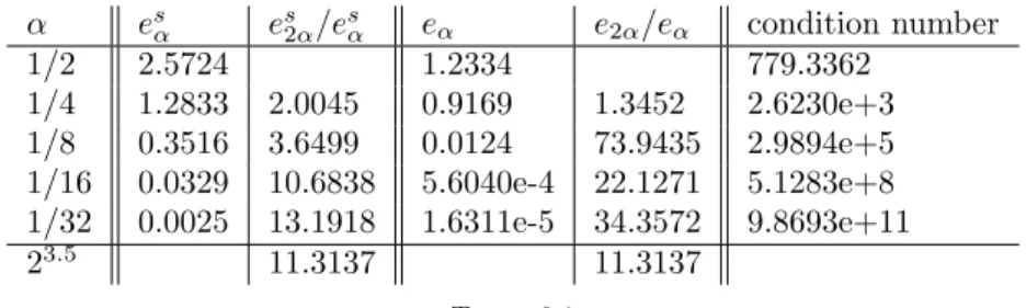
In each case we have calculated the errors eα= max x∈Xcheck kSα(x)−M(x)kmax= max x∈Xcheck max i,j=1,2|S α ij(x)−Mij(x)| esα= max x∈Xcheck kF(Sα)(x)−F(M)(x)kmax, 17
withXcheck={(x, y)∈R2:x, y=−1+12α0, . . . ,− 3 2α0,− 1 2α0, 1 2α0, 3 2α0, . . . ,1− 1 2α0} withα0= 216. By Theorem 5.3 we expect the errors to behave like
e2α eα
≈2σ−1−n/2= 23.5.
Table 6.1 shows the above described errors for different α, the expected ratios and the condition numbers of the collocation matrices. The expected approximation order is well-matched by the observed errorF(S)−F(M). In the case ofS−M, the observed error is signficantly better than predicted.
α esα es2α/esα eα e2α/eα condition number 1/2 2.5724 1.2334 779.3362 1/4 1.2833 2.0045 0.9169 1.3452 2.6230e+3 1/8 0.3516 3.6499 0.0124 73.9435 2.9894e+5 1/16 0.0329 10.6838 5.6040e-4 22.1271 5.1283e+8 1/32 0.0025 13.1918 1.6311e-5 34.3572 9.8693e+11 23.5 11.3137 11.3137 Table 6.1
Errors for various computation grids together with the error behaviour and the condition number of the collocation matrix.
Next, we have fixed the grid to consist of the N = 1681 points X ={(x, y) ∈
R2 : x, y = −4,−3.8,−3.6, . . . ,0,0.2, . . . ,4}. As each grid point requires 3 vari-ables of a symmetric 2×2 matrix, we solve a linear system with a 5043×5043 matrix; its condition number is 1.6419e+5. We need to check that the constructed matrix-valued functionS(x) is positive definite andF(S)(x) is negative definite, where F(S) =Df(x)TS(x) +S(x)Df(x) +S0(x). To check that a 2×2 matrix A is
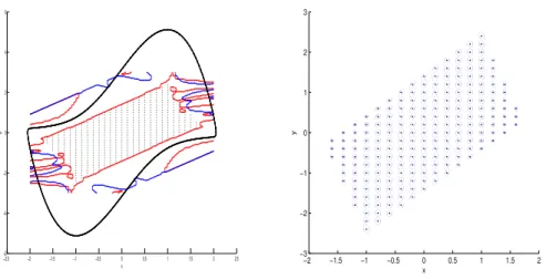
pos-itive/negative definite it suffices to check that tr(A) is positive/negative and det(A) is positive/−det(A) is negative. For this example, trS(x), detS(x) are positive in the whole area [−4,4]2, while Figure 6.1, left, shows small areas near the boundary where F(S)(x) is not negative definite, together with the collocation points. Fig-ure 6.1, right, illustrates the metric S(x) by plotting ellipses x+v around x with (v−x)TS(x)(v−x) =const, showing that S(x) approximates the constant solution (6.1) well.
6.2. Van der Pol. We consider the van der Pol system with reversed time, which has an exponentially stable equilibrium at the origin. Its basin of attraction is bounded by an unstable periodic orbit. The system is given by
˙
x=−y, y˙ =x−3(1−x2)y,
which was, for example, considered in [19] to compute a Lyapunov function. In our computations, we have used C = I and the grid X = {(x, y) ∈ R2 | x, y = . . . ,−0.25,−0.125,0,0.125, . . .} ∩ {x−1.5< y <1.5 +x,−3x−5.5< y <−3x+ 5.5}
with N = 501 points, and as each grid point requires 3 variables of a symmetric 2×2 matrix, we have solved a linear system with a 1503×1503 matrix; the condition number is 3.0024e+6. We have used the same kernel as in the previous example.
Figure 6.3, left, shows the collocation points and the basin of attraction of the origin, bounded by an unstable periodic orbit as well as the boundaries of the areas whereF(S)(x) is negative definite (red) andS(x) is positive definite (blue).
−4 −3 −2 −1 0 1 2 3 4 −4 −3 −2 −1 0 1 2 3 4 x y −5 −4 −3 −2 −1 0 1 2 3 4 5 −5 −4 −3 −2 −1 0 1 2 3 4 5 x y
Fig. 6.1. Left: The collocation points used for the RBF approximation together with the areas
whereF(S)(x, y)is not negative definite (red). Right: To illustrate the approximationS, around
some pointsx, we have plotted the curve of equal distance with respect to metricS(x), in particular
the set{x+v|(v−x)TS(x)(v−x) = const}.
−2 −1 0 1 2 −3 −2 −1 0 1 2 3 −2 0 2 x y −2 −1 0 1 2 −4 −2 0 2 4 −2 −1.5 −1 −0.5 0 0.5 1 1.5 2 x y
Fig. 6.2.Left: sign(trF(S)(x, y))−sign(detF(S)(x, y)). If this function is−2, thenF(S)(x, y)
is negative definite. Right: sign(trS(x, y)) + sign(detS(x, y)). If this function is+2, thenS(x, y)is
positive definite.
In more detail, Figure 6.2 shows sign(trF(S)(x))−sign(detF(S)(x)), which is
−2 in the area where we placed the collocation points (left), as well as sign(trS(x)) + sign(detS(x)) which is +2 in the area where we placed the collocation points (right). Figure 6.3, right, shows the point-dependent metric S(x) by plotting ellipses x+v aroundxwith (v−x)TS(x)(v−x) =const.
REFERENCES
[1] L. Amodei,Reproducing kernels of vector-valued function spaces, in Surface Fitting and
Mul-tiresolution Methods, A. L. M´ehaut’e, C. Rabut, and L. L. Schumaker, eds., Nashville, 19
−2.5 −2 −1.5 −1 −0.5 0 0.5 1 1.5 2 2.5 −6 −4 −2 0 2 4 6 x y −2 −1.5 −1 −0.5 0 0.5 1 1.5 2 −3 −2 −1 0 1 2 3 x y
Fig. 6.3. Left: Collocation points and the boundary of the basin of attraction of the origin,
an unstable periodic orbit, together with the boundaries of the areas where sign(trF(S)(x, y))−
sign(detF(S)(x, y)) =−2(red) and sign(trS(x, y)) + sign(detS(x, y)) = 2(blue). Right: To
illus-trate the approximation S, around some points x, we have plotted the set of equal distance with
respect to metricS(x), in particular the set{x+v|(v−x)>S(x)(v−x) = const}.
1997, Vanderbilt University Press, pp. 17–26.
[2] N. Aronszajn,Theory of reproducing kernels, Trans. Am. Math. Soc., 68 (1950), pp. 337–404.
[3] E. M. Aylward, P. A. Parrilo, and J.-J. Slotine, Stability and robustness analysis of
nonlinear systems via contraction metrics and SOS programming, Automatica, 44 (2008),
pp. 2163–2170.
[4] M. N. Benbourhim and A. Bouhamidi,Meshless pseudo-polyharmonic divergence-free and
curl-free vector fields approximation, SIAM J. Math. Anal., 42 (2010), pp. 1218–1245.
[5] A. Berlinet and C. Thomas-Agnan,Reproducing Kernel Hilbert Spaces in Probability and
Statistics, Springer, New York, 2004.
[6] G. Borg, A condition for the existence of orbitally stable solutions of dynamical systems,
vol. 153 of Kungl. Tekn. H¨ogsk. Handl., Elander, 1960.
[7] M. D. Buhmann,Radial Basis Functions, Cambridge Monographs on Applied and
Computa-tional Mathematics, Cambridge University Press, Cambridge, 2003.
[8] B. Burgeth, S. Didas, L. Florack, and J. Weickert, A generic approach to diffusion
filtering of matrix-fields, Computing, 81 (2007), pp. 179–197.
[9] C. Chefd’hotel, D. Tschumperl´e, R. Deriche, and O. Faugeras,Constrained flows of
matrix-valued functions: Application to diffusion tensor regularization, in Computer
Vi-sion — ECCV 2002: 7th European Conference on Computer ViVi-sion Copenhagen, Denmark, May 28–31, 2002 Proceedings, Part I, A. Heyden, M. Sparr, Gunnarand Nielsen, and P. Jo-hansen, eds., Springer Berlin Heidelberg, Berlin, Heidelberg, 2002, pp. 251–265.
[10] N. Cristianini and J. Shawe-Taylor,An introduction to support vector machines and other
kernel-based learning methods, Cambridge University Press, Cambridge, 2000.
[11] F. Cucker and S. Smale,On the mathematical foundation of learning, Bull. Amer. Math.
Soc., 39 (2002), pp. 1–49.
[12] J. Dick, F. Y. Kuo, and I. H. Sloan,High-dimensional integration: The quasi-Monte Carlo
way, in Acta Numerica, A. Iserles, ed., vol. 22, Cambridge University Press, 2013, pp. 133– 288.
[13] G. Fasshauer,Meshfree Approximation Methods with MATLAB, World Scientific Publishers,
Singapore, 2007.
[14] N. Flyer and B. Fornberg,Radial basis functions: Developments and applications to
plan-etary scale flows, Computers and Fluids, 46 (2011), pp. 23–32.
[15] B. Fornberg and N. Flyer, Solving PDEs with radial basis functions, in Acta Numerica,
A. Iserles, ed., vol. 24, Cambridge University Press, 2015, pp. 215–258.
[16] F. Forni and R. Sepulchre, A differential Lyapunov framework for contraction analysis,
IEEE Transactions on Automatic Control, 59 (2014), pp. 614–628. 20
[17] C. Franke and R. Schaback,Convergence order estimates of meshless collocation methods
using radial basis functions, Adv. Comput. Math., 8 (1998), pp. 381–399.
[18] E. Fuselier,Sobolev-type approximation rates for divergence-free and curl-free RBF
inter-polants, Math. Comput., 77 (2008), pp. 1407–1423.
[19] P. Giesl,Construction of global Lyapunov functions using radial basis functions, vol. 1904 of
Lecture Notes in Mathematics, Springer-Verlag, Heidelberg, 2007.
[20] ,Converse theorems on contraction metrics for an equilibrium, J. Math. Anal. Appl.,
424 (2015), pp. 1380–1403.
[21] P. Giesl and S. Hafstein,Construction of a CPA contraction metric for periodic orbits using
semidefinite optimization, Nonlinear Anal., 86 (2013), pp. 114–134.
[22] P. Giesl and S. Hafstein,Computation and verification of Lyapunov functions, SIAM J.
Appl. Dyn. Syst., 14 (2015), pp. 1663–1698.
[23] ,Review on computational methods for Lyapunov functions, Discrete and Continuous
Dynamical Systems - Series B (DCDS-B), 20 (2015), pp. 2291 – 2331.
[24] P. Giesl and H. Wendland, Meshless collocation: Error estimates with application to
dy-namical systems, SIAM J. Numer. Anal., 45 (2007), pp. 1723–1741.
[25] , Construction of a contraction metric by meshless collocation. Preprint
Bayreuth/Sussex, to appear in Discrete and Continuous Dynamical Systems Series B, 2016.
[26] W. Hahn,Stability of Motion, Springer, Berlin, 1967.
[27] P. Hartman,Ordinary Differential Equations, Wiley, New York, 1964.
[28] E. J. Kansa, Multiquadrics - A scattered data approximation scheme with applications to
computational fluid-dynamics I. Surface approximations and partial derivative estimates,
Comput. Math. Appl., 19 (1990), pp. 127–145.
[29] H. Khalil,Nonlinear systems, Macmillan Publishing Company, New York, 1992.
[30] N. N. Krasovskii,Problems of the Theory of Stability of Motion, Mir, Moscow, 1959.
[31] G. A. Leonov, I. M. Burkin, and A. I.Shepelyavyi,Frequency Methods in Oscillation
The-ory, vol. 357 of Ser. Math. and its Appl., Kluwer, 1996.
[32] W. Lohmiller and J.-J. E. Slotine,On contraction analysis for non-linear systems,
Auto-matica J. IFAC, 34 (1998), pp. 683–696.
[33] S. Lowitzsch, Approximation and Interpolation Employing Divergence-Free Radial Basis
Functions with Applications, PhD thesis, Texas A&M University, College Station, USA,
2002.
[34] S. Mardare,On systems of first order linear partial differential equations withLpcoefficients,
Adv. Differential Equations, 12 (2007), pp. 301–360.
[35] C. A. Micchelli and M. Pontil,Learning the kernel function via regularization, J. of Mach.
Learning Research, 6 (2005), pp. 1099–1125.
[36] F. J. Narcowich and J. D. Ward,Generalized Hermite interpolation via matrix-valued
con-ditionally positive definite functions, Math. Comput., 63 (1994), pp. 661–687.
[37] F. J. Narcowich, J. D. Ward, and H. Wendland,Sobolev bounds on functions with scattered
zeros, with applications to radial basis function surface fitting, Math. Comput., 74 (2005),
pp. 643–763.
[38] R. Schaback,The missing Wendland functions, Adv. Comput. Math., 34 (2011), pp. 67–81.
[39] R. Schaback and H. Wendland, Kernel techniques: From machine learning to meshless
methods, in Acta Numerica, A. Iserles, ed., vol. 15, Cambridge University Press, 2006,
pp. 543–639.
[40] B. Sch¨olkopf and A. J. Smola,Learning with Kernels – Support Vector Machines,
Regular-ization, OptimRegular-ization, and Beyond, MIT Press, Cambridge, Massachusetts, 2002.
[41] I. Steinwart and A. Christmann,Support Vector Machines, Springer, New York, 2008.
[42] B. Stenstr¨om,Dynamical systems with a certain local contraction property, Math. Scand., 11
(1962), pp. 151–155.
[43] V. Vapnik,Statistical Learning Theory, John Wiley and Sons, 1998.
[44] J. Weickert and T. Brox,Diffusion and regularization of vector- and matrix-valued images,
in Inverse problems, image analysis, and medical imaging (New Orleans, LA, 2001), vol. 313 of Contemp. Math., Amer. Math. Soc., Providence, RI, 2002, pp. 251–268.
[45] H. Wendland,Piecewise polynomial, positive definite and compactly supported radial functions
of minimal degree, Adv. Comput. Math., 4 (1995), pp. 389–396.
[46] , Meshless Galerkin methods using radial basis functions, Math. Comput., 68 (1999),
pp. 1521–1531.
[47] ,Scattered Data Approximation, Cambridge Monographs on Applied and Computational
Mathematics, Cambridge University Press, Cambridge, UK, 2005.
[48] ,Divergence-free kernel methods for approximating the Stokes problem, SIAM J. Numer.
Anal., 47 (2009), pp. 3158–3179.