Statistical Methods for Dealing with Selective Crossover in Randomised Controlled Trials

(1)

Alma Mater Studiorum – Università di Bologna

DOTTORATO DI RICERCA IN

METODOLOGIA STATISTICA PER LA RICERCA SCIENTIFICA

Ciclo XXVII

Settore Concorsuale di afferenza: 13/D1

Settore Scientifico disciplinare: SECS-S/02

STATISTICAL METHODS FOR DEALING WITH

SELECTIVE CROSSOVER IN RANDOMISED CONTROLLED TRIALS

Candidata: Dott.ssa Sara Balduzzi

Coordinatrice Dottorato

Relatrice

Prof.ssa Alessandra Luati

Prof.ssa Rossella Miglio

Correlatore

Prof. Roberto D’Amico

(2)

(3)

Acknowledgements

First of all, special thanks go to Prof. Rossella Miglio and Prof. Roberto D’Amico, for having given me the opportunity to work on this project: I hope to keep on working with you, your support, guidance, patience and understanding on this and many other projects in the future.

I want to thank Dr. Elisabetta Petracci, who offered me her precious help from the beginning.

Elisabetta, Linda, Giovanni, Elena, Arianna: it was an honour (and pretty fun!) to share this path with you.

My life at work, which I love, would not be the same without my beautiful colleagues: Cinzia, Elena, Nika, Roberto V. Thank you for your support and for listening to me every time I need it.

An important thank goes to my parents – I know you are my biggest fans.

Thanks to Alberto, especially for letting me buy a desk and a shelf: without them it would have been much more difficult to write this thesis.

Last four years have surely been the most intense ones of my life. I would like to thank all the people who walked by my side, at least for a moment, during this period.

(5)

Introduction

The evidence to support the efficacy and safety of a drug derives from randomised controlled trials (RCTs) [1]. The ethical basis of a RCT is provided by the principle of equipoise, stating that the randomization is allowed when there is genuine uncertainty on the actual benefit of the intervention under study.

An RCT ideally should permit an unbiased estimation of the treatment effect (e.g., overall survival (OS) or disease-free survival (DFS)), through the comparison between an experimental treatment and a comparator, administrated in two separate arms. However, sometimes patients may be offered the possibility to cross over from one arm of the trial to the other, a phenomenon usually called selective crossover (SCO), in order to distinguish it from the studies in which crossover is planned. Other terms to refer to this switch are drop-in or cross-drop-in [2]. It can occur as a consequence of the diffusion of (un)favourable results of one treatment that is being compared, e.g. from interim analysis or from concurrent studies. In both cases the equipoise principle is challenged. If so, the investigators may offer patients the opportunity to cross over to the arm where the more promising treatment is administered.

This thesis considers treatment crossover as the switching of patients randomised to the control group of an RCT on to the experimental treatment, at a certain point after randomisation.

The occurrence of SCO breaks the randomization process and may give rise to problems in the data analysis and interpretation of results. In fact, in presence of SCO, the Intention to Treat (ITT) analysis, that is the analysis considering groups as randomised, will give an unbiased estimate of the experimental treatment assignment effect, but that effect will also

(6)

include the one of the experimental treatment administered to patients in the control group who switched. So the results of this type of analysis may not reflect the actual efficacy of the experimental intervention, and adjustments to allow for crossover are needed.

My personal interest in this topic derives from the work that I conducted for my master degree thesis, when I presented the results of a systematic review on the efficacy and safety of a drug, i.e. trastuzumab, for the treatment of early and metastatic breast cancer. The work of my colleagues and me has been published in two articles [3,4]. In both adjuvant/neoadjuvant and metastatic settings, we observed that more than half of the included studies let patients in the control arm cross over to the trastuzumab arm at a certain point after randomisation. While in the metastatic setting crossover was permitted generally after progression, making it difficult to estimate the actual benefit of trastuzumab on OS, in the adjuvant/neoadjuvant setting it was permitted before disease progression, making it difficult to analyse and interpret both OS and DFS results.

The present work aims to:

(i) assess the prevalence of SCO in RCTs assessing the efficacy and safety of biological and hormonal therapies for breast cancer and published in the scientific literature;

(ii) identify the reported statistical methods used to handle crossover, in particular when the effect of the experimental treatment is a time-to-event outcome; (iii) assess whether different statistical methods provide different results and

(7)

Overview of the thesis

Chapter 1 presents the review of the medical scientific literature carried out in order to assess the prevalence of the SCO in the field of breast cancer, and the approaches adopted to handle it. Details on the methods adopted to conduct the review are given, along with the presentation of the results, distinguished for adjuvant/neoadjuvant and metastatic setting. The Chapter closes with a discussion regarding the findings of the review and the needs for further research.

Chapter 2 attempts to collect the more relevant approaches that have been considered in literature to address treatment crossover.

Along with ITT analysis, other naïve methods include censoring patients at the time they cross over, or excluding them from the analysis. These methods will lead to biased results if the switching process is not random, because of selection bias. If patients who switch are picked completely at random, their exclusion from the analysis would not result in bias, but in the loss of power and increase of the uncertainty in the results. Instead, a switching process depending on patients’ characteristics implies informative censoring, and censoring or excluding from the analysis patients who cross over will lead to biased results.

Another method described in literature is to consider the treatment as a time-varying covariate. This approach may be subject to selection bias, as groups may no longer be balanced after a patient is censored or excluded, and bias is likely if a patient’s probability of switching treatment is related to their underlying prognosis.

Morden et al. [5] studied some statistical approaches for dealing with SCO. They considered naïve methods, as well as more complex ones, such as Robins and Tsiatis’s Rank Preserving Structural Failure Time Model (RPSFTM) [6]. The key assumption, though not always reasonable, of the RPSFTM method is the so-called “common treatment

(8)

effect” assumption: it is assumed that switching patients experience the same treatment effect, from the time they start taking the experimental treatment, as patients randomised to the experimental group from the beginning.

Another approachconsidered in the paper by Morden et al., and evaluated in this thesis, is the one described in Loeys and Goetghebeur [8], who present a method for calculating the actual treatment effect in situations where all patients take their allocated treatment in one group, and compliance is assumed as “all-or-nothing” in the other. So, if a patient in this arm cross over, the switch is assumed to have happened right after the randomisation, and the patient is assumed to have only received the treatment he/she switched onto and not the treatment he/she was randomised to.

The inverse probability of censoring weights (IPCW) method, introduced by Robins and Finkelstein [9], not evaluated in the paper by Morden et al., is also considered in the present work. The IPCW method do not assume the “common treatment effect”, but its fundamental assumption is the “no unmeasured confounders”, that is the requirement of data on all covariates that might influence the crossover.

All these methods are presented in Chapter 2 of this thesis.

In order to assess the potential bias associated with the methods described in Chapter 2, the actual effect of an intervention under study needs to be known, so a simulation study was performed. The idea was to reproduce a two-arm RCT, similar to one of the trials emerged from the review of the literature of Chapter 1: this work focuses the attention on the adjuvant/neoadjuvant setting, where the crossover is usually permitted before disease recurrence. Chapter 3 details the simulation study design and Chapter 4 presents the results.

(9)

Chapter 1

Review of the literature

In this chapter it is presented the review of the scientific literature conducted in order to evaluate the prevalence of the SCO among trials evaluating the efficacy and safety of the biological drugs and hormonal therapies for breast cancer, and the statistical methods used to handle it.

1.1.Methods

RCTs (phase III only) published between January 2000 and June 2015 in the Annals of Oncology (AoO), Journal of Clinical Oncology (JCO), Journal of the National Cancer Institute (JNCI), Lancet (L), Lancet Oncology (LO), New England Journal of Medicine (NEJM), assessing the efficacy and safety of biological drugs and hormonal therapy in breast cancer patients, were searched. We excluded chemotherapy agents because, in those years we selected as study time period, there were few new agents granting marketing authorisation: last innovative agents – doxorubicin pegylated and paclitaxel – were approved by the European Medicine Agency in 2000 [9].

The keywords used for the research were “random*”, “breast” and “cancer” – with the restriction that all words had to be present in the title or in the abstract.

Trials were distinguished by the therapy setting they considered, i.e. adjuvant/neoadjuvant or metastatic. The prevalence was calculated as the percentage of trials in which crossover has occurred out of the total number of trials reflecting the inclusion criteria.

For trials in which crossover has occurred, the following characteristics were recorded: primary end point, reason for crossover (i.e. interim analysis), number of patients totally

(10)

randomized, number and type of patients allowed to cross over, statistical methods used to analyse results after the crossover. When reported, characteristics of patients who crossed over in respect to patients who remained in the arm of original allocation was also recorded.

If a trial reported the results for the same outcome (i.e. for overall survival (OS) or disease/progression-free survival (DFS/PFS)) in terms of hazard ratios (HR) from more than one type of analysis, the ratio of HRs (RHR), along with its 95% confidence interval (95%CI) was calculated in order to compare them.

1.2. Results

Figure 1. Flowchart of the bibliographic research

1706 references

From 6 journals: NEJM, JNCI, Lancet, Lancet Oncology, JCO, Annals of Oncology

Period limits: January 2000-June 2015

351 references reporting the results of phase III or “uncertain phase” RCTs – full text retrieved

128references reporting the results of 85

phase III RCTs:

- 42 in a metastatic setting;

- 43 in an adjuvant/neoadjuvant setting

1355 references excluded because they considered non-pertinent topics or because they considered phase II studies

202 references excluded because the interventions were neither biological nor hormonal

(11)

The flowchart of the literature research is presented in Figure 1. Out of 1706 references totally retrieved (AoO 434; JCO 553; JNCI 192; L or LO 104; NEJM 423), 1355 were excluded because they did not consider treatments for breast cancer or because they considered phase II studies. The full text of the remaining 351 references was retrieved: 202 were then excluded because the interventions were therapies neither biological nor hormonal and 21 because the study phase was unclear. The remaining 128 references reported the results of 85 RCTs, 43 of which enrolled women in early breast cancer and 42 metastatic.

Crossover was present in 20 RCTs (23.5%) equally distributed across settings: ten in adjuvant/neoadjuvant settings (23.3%) and ten in metastatic setting (23.8%).

When SCO occurred, the methods used to analyse data were: 1. Intention To Treat (ITT) analysis;

2. Censored analysis;

3. Inverse Probability of Censoring Weighting (IPCW) analysis.

In the ITT analysis, controls that crossed over are analysed as belonging to the control arm, despite the fact that they crossed over to the treatment intervention.

In the censored analysis, follow-ups of controls that switched to the intervention arm are censored at the time when the crossover occurred.

The IPCW analysis allows the estimation of the missing follow-ups of those controls who switched arm by using the information comprised in follow-ups of those controls who instead decided against crossing over and who were similar in terms of prognostic factors to their counterparts [8].

(12)

1.2.1. Adjuvant/Neoadjuvant setting

Characteristics of the ten RCTs (IMPACT, HERA, MA17, NSABP-B-33, BIG 1-98, NOAH, BCIRG-006, TEAM, B31, N9831) assessing efficacy and safety of treatments in the adjuvant/neoadjuvant setting in which SCO occurred are shown in Table 1.a. The studies B31 and N9831 were analysed and presented jointly, because they evaluate the same intervention, administered on a similar schedule. Five trials evaluated biological drugs and five hormonal therapies. Nine trials had DFS as primary outcome, one (IMPACT) had clinical tumour overall response. OS was always a secondary outcome. Two trials (IMPACT, NOAH) considered neoadjuvant strategies, and these are the trials with the lowest number of randomized patients (330 and 334 respectively). In five big trials (BIG 1-98, HERA, MA17, B31+N9831, with 8010, 3401, 5170, and 4390 randomized patients respectively), crossover was allowed after positive results obtained at a pre-planned interim analyses. HERA and MA17 were the trials with the highest percentage of patients crossing over, 52% and 61% respectively. In three trials (IMPACT, NSABP-B-33, TEAM) patients were permitted to cross over after results from other similar studies were published leading to a protocol amendment. For two trials (BCIRG-006, NOAH) the motivation for crossover was not reported. These trials had the lowest percentage of patients crossed over, 2.1% and 16% respectively. Other two trials (IMPACT, TEAM) did not clearly report the percentage of patients who crossed over. In two trials (BIG 1-98, HERA) the crossover was allowed only to patients who did not experience recurrence yet (HERA also required an adequate left ventricular ejection fraction); in the other studies, the crossover seemed to be offered to all patients in the control arm.

(13)

censored analyses were published and in 2011 another paper reported an update of the ITT analysis and the IPCW analysis.

Only two trials (HERA, MA17) reported the characteristics – in terms of age, previous therapy, menopausal status, hormone-receptor status, and lymph nodal status – of patients of the control arms who crossed over to the treatment arms, along with the characteristics of patients who did not. In both cases, patients in the SCO cohort compared with patients remaining in the control arm were more likely to be younger and have hormone-receptor-positive disease.

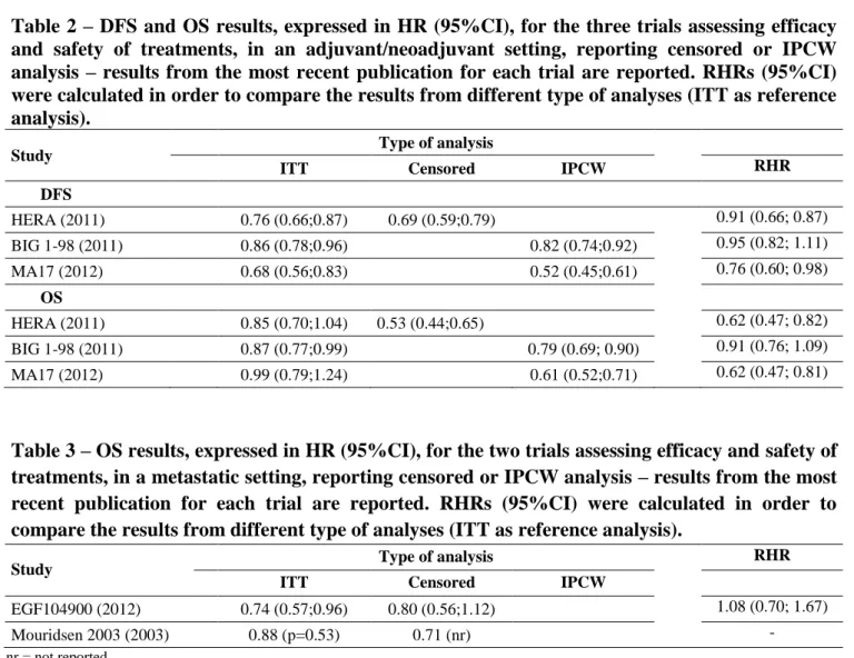
In table 2 are reported the results, expressed in HR (95%CI), for the three trials reporting censored or IPCW analysis, for DFS and OS respectively. The ITT analysis always seemed to be the more conservative one, although for the BIG 1-98 trial the RHRs both for OS and DFS were not statistically significant. OS results deriving from censored or IPCW analyses were more distant from the ones obtained with the ITT analysis in respect to DFS results.

1.2.2. Metastatic setting

Characteristics of the ten RCTs (Slamon 2001, Mouridsen 2003, TANDEM, AVADO, EGF104900, RIBBON-1, NCT00435409, NCT00938652, NCT00075764, CONFIRM) assessing efficacy and safety of treatments for metastatic breast cancer in which SCO occurred are shown in Table 1.b. All the trials but three (Mouridsen 2003, NCT00075764, CONFIRM) evaluated biological drugs. All the trials considered PFS as primary outcome and OS as secondary outcome.

All the trials’ protocols permitted crossover to the experimental treatment arm for a patient in the control arm who experienced progression. RIBBON-1 was a four-arms trial, two controls and two experimental arms; after progression, patients in both the control arms were permitted to switch to the respective experimental arm. A particular case is represented by the Mouridsen 2003 trial, where two different hormonal therapies were

(14)

compared and in which patients at progression were permitted to switch to the other arm, irrespective of the arm in which they were initially allocated.

The percentages of switched patients were over the 40% in all the studies but three (AVADO 36%, NCT00435409 36%, CONFIRM 2%). All the studies reported the ITT analysis and two (EGF104900, Mouridsen 2003) conducted censored analysis.

Only one study (EGF104900) reported the main characteristics – age, performance status, prior therapies, hormone-receptor status – of the control arm by crossover status (crossover versus non-crossover), without statistically evaluating the differences between the two groups.

In table 3 are reported the OS results, expressed in HR, for the two trials reporting censored analysis. Mouridsen 2003 calculated the median time to death in each group, from which it was possible to estimate the HR; too less information was provided to calculate the RHR. The HRs from the ITT and the censored analyses reported by the EGF104900 trial do not seem to differ significantly.

(15)

Table 1.a – Characteristics of the trials in which SCO occurred – Trials assessing efficacy of treatments in an adjuvant/neoadjuvant setting Study BD/ HT Journal Year of publication* Year of reported SCO Primary End Point Motivation for SCO Pts totally randomized/ to be enrolled

Pts crossed over ITT Cens IPCW

1 IMPACT° HT JCO 2005 2005 Clinical tumour

OR

After ATAC

results 330/330 Not reported √

2 HERA BD NEJM,L,LO 2005-2011 2007 DFS Interim analysis 5102/4482 885/1698 (52%) √ √

3 MA17 HT JCO,AoO,NEJ M 2003-2012 2008 DFS Interim analysis, unblinding 5187/4800 1579/2587 (61%) √ √ 4 NSABP-B-33 HT JCO 2008 2008 DFS After MA17 (interim analysis) results 1598/3000 344/779 (44%) √

5 BIG 1-98 HT NEJM,JCO,LO 2005-2011 2009 DFS Planned interim

analysis 8010/8028 619/2459 (25%) √ √ √

6 NOAH° BD L 2010 2010 DFS (EFS) Not reported 235/232 19/118 (16%) √

7 BCIRG-006 BD NEJM 2011 2011 DFS Not reported 3222/3150 23/1073 (2.1%) √

8 TEAM HT L 2011 2011 DFS After IES results 9779/9300 Not reported √

9+

10 B31+N9831 BD NEJM,JCO 2005-2014 2014 DFS

Planned interim

analysis 4390/4130 413/2018 (20%) √

* If more than one publication refers to the same study, the year of first publication and the year of last publication are reported Pts=patients

NEJM=New England Journal of Medicine; JNCI=Journal of the National Cancer Institute; L=Lancet; LO=Lancet Oncology; JCO=Journal of Clinical Oncology; AoO=Annals of Oncology DFS=Disease Free Survival; OR=Objective Response

HT=Hormonal therapy; BD=Biological Drug

(16)

Table 1.b – Characteristics of the trials in which SCO occurred – Trials assessing efficacy of treatments in a metastatic setting Study BD/ HT Journal Year of publication* Year of reported SCO Primary End Point Motivation for SCO Pts totally randomized/ to be enrolled

Pts crossed over ITT Cens IPCW

1 Slamon 2001 BD NEJM 2001 2001 PFS After progression 469/450 154/234 (66%) √

2 Mouridsen

2003 HT JCO 2003 2003 PFS After progression 907/907

233/458 (51%) +

226/458 (49%) √ √

3 TANDEM BD JCO 2009 2009 PFS After progression 208/208 73/104 (70%) √

4 AVADO BD JCO 2010 2010 PFS After progression 736/705 83/231 (36%) √

5 EGF104900 BD JCO 2010-2012 2010 PFS After progression 296/296 77/145 (53.1%) √ √

6 RIBBON-1 BD JCO 2011 2011 PFS After progression 1237/1200 112/206 (54.4%) +

105/207 (50.7) √

7 NCT00435409 BD JCO 2013 2013 PFS After progression 432/430 77/215 (36%) √

8 NCT00938652 BD JCO 2014 2014 PFS After progression 519/420 161/258 (62%) √

9 NCT00075764 HT NEJM 2012 2012 PFS After progression 695/690 143/345 (41%) √

10 CONFIRM HT JNCI 2014 2014 PFS After progression 736/834 8/374 (2%) √

* If more than one publication refers to the same study, the year of first publication and the year of last publication are reported Pts=patients

NEJM=New England Journal of Medicine; JNCI=Journal of the National Cancer Institute; L=Lancet; LO=Lancet Oncology; JCO=Journal of Clinical Oncology; AoO=Annals of Oncology PFS=Progression Free Survival; EFS=Event Free Survival

HT=Hormonal therapy; BD=Biological Drug

(17)

Table 2 – DFS and OS results, expressed in HR (95%CI), for the three trials assessing efficacy and safety of treatments, in an adjuvant/neoadjuvant setting, reporting censored or IPCW analysis – results from the most recent publication for each trial are reported. RHRs (95%CI) were calculated in order to compare the results from different type of analyses (ITT as reference analysis).

Study Type of analysis

ITT Censored IPCW RHR

DFS HERA (2011) 0.76 (0.66;0.87) 0.69 (0.59;0.79) 0.91 (0.66; 0.87) BIG 1-98 (2011) 0.86 (0.78;0.96) 0.82 (0.74;0.92) 0.95 (0.82; 1.11) MA17 (2012) 0.68 (0.56;0.83) 0.52 (0.45;0.61) 0.76 (0.60; 0.98) OS HERA (2011) 0.85 (0.70;1.04) 0.53 (0.44;0.65) 0.62 (0.47; 0.82) BIG 1-98 (2011) 0.87 (0.77;0.99) 0.79 (0.69; 0.90) 0.91 (0.76; 1.09) MA17 (2012) 0.99 (0.79;1.24) 0.61 (0.52;0.71) 0.62 (0.47; 0.81)

Table 3 – OS results, expressed in HR (95%CI), for the two trials assessing efficacy and safety of treatments, in a metastatic setting, reporting censored or IPCW analysis – results from the most recent publication for each trial are reported. RHRs (95%CI) were calculated in order to compare the results from different type of analyses (ITT as reference analysis).

Study Type of analysis RHR

ITT Censored IPCW

EGF104900 (2012) 0.74 (0.57;0.96) 0.80 (0.56;1.12) 1.08 (0.70; 1.67)

Mouridsen 2003 (2003) 0.88 (p=0.53) 0.71 (nr) -

(18)

1.3.Review findings

Between January 2000 and June 2015, one out of five RCTs assessing efficacy of innovative biological drugs and hormonal therapy for breast cancer permitted patients to cross over at a certain point during the course of the study. From a clinical standpoint, early discontinuation of RCT due to unequivocal observed benefit, harm or futility are always justified by ethical issues. An early interruption for benefit leads to stopping further recruitment in a potential inferior arm, and patients randomized to the control arm can opt to cross over to receive the experimental treatment. However, from a methodological standpoint, this approach leads to uncertainties surrounding the true magnitude of the actual effect.

The scenario might be different when considering the early or the advanced disease setting. Indeed, it is well accepted that patients with metastatic disease, at the time of disease progression, are given the opportunity to switch to the arm with the more promising therapy. This approach has no effect on the earlier measures of treatment effect such as PFS, which represents the primary outcome in all the found studies. On the other hand, the crossover can definitively preclude the possibility to demonstrate an OS benefit, which is often considered the ultimate test of efficacy.

The situation is even more critical in the adjuvant setting, where SCO is generally offered to patients still free of disease recurrence, thus affecting the clear interpretation of both DFS and OS. The scientific community has to deal with the ethical imperative to offer the best treatment to those patients who decide to enter a clinical trial, and with the need of obtaining the most clean evidence to be applied in the whole population. Indeed, all the

(19)

All the studies included in the present analysis were always analyzed following the ITT approach, which is the traditional analysis. According to the ITT principle, patients are analysed in their assigned treatment arm regardless of the actual treatment received. Therefore, when a substantial fraction of the patients from the less active treatment cross to the more effective treatment, the net benefit of the latter tends to be reduced. Censored analysis can be used to account for disruptions in treatment allocation. This approach censures patients after crossover, and can be more informative on the real performance of the experimental arm. Only 2/10 adjuvant and 2/10 metastatic studies included in the present analysis reported the censored analysis. The censored analysis was associated with an increased benefit for the experimental arm as compared to the ITT analysis. However, censored analysis can introduce bias itself, in particular when censored patients are more likely or less likely to experience the event than uncensored patients (informative censoring). In both HERA and MA17 trials, patients in the SCO cohort were more likely to be younger and have hormone-receptor-positive disease, as compared to patients remaining in the control arm.

One of the most recent type of analysis, IPCW [8], which accounts for prognostic factors, was rarely used (2/10 adjuvant trials). Similarly to the censored analysis, IPCW analysis led to results which favour the experimental arm in respect to the ITT analysis, which instead tends to dilute the treatment effect. By the way, the adjustment made by the IPCW analysis is valid only if the variables which determine crossover are known and measurable, as pointed out by Rimawi et al. [10]. This is not always possible, leaving the choice to imply this type of analysis doubtful.

The main limitation of the research presented in this chapter is the fact that only articles that appeared within a 15-year period were searched in six selected medical journals, reasoning that these ones published most of the RCTs in breast cancer. It would be helpful to further investigate the phenomenon with a more comprehensive literature research. The

(20)

prevalence and impact of SCO in fields other than breast cancer should also be studied. The magnitude and direction of the potential bias introduced by the SCO needs to be clearly evaluated, as well as the impact on the results for different effect sizes when results concern safety and when the reason for switching depends on a combination of prognostic factors.

However, the lack of an appropriate reporting is not a trivial concern. In 2005, Montori et al. published a systematic review of RCTs stopped early for benefit [11], which might lead to SCO, in which they highlighted the lack of adequately reported such an important information as the motivation to stop the trial. More attention should be paid by the authors also in the reporting of the characteristics of patients to whom the crossover is offered. Considering the increasing frequency of the phenomenon, the Consolidated Standards of Reporting Trials (CONSORT) statement [1] could be modified in order to recommend the specification of that information, fundamental for a better understanding and interpretation of the results of the trial.

This chapter clearly points out that the treatment crossover phenomenon is quite common in breast cancer trials. Different methods may lead to different results and interpretations, but there is still no consensus on the appropriate approach to deal with SCO.

(21)

Chapter 2

Methods for dealing with selective cross over

Chapter 1 highlighted the need to find appropriate strategies to deal with treatment crossover.

The present chapter describes the most relevant existing statistical approaches to handle SCO. These methods will be then assessed through simulation, as explained in Chapter 3, and the results of the simulations will be presented in Chapter 4.

2.1.Naïve methods

2.1.1. Intention-to-treat (ITT) analysis

As emerged from the medical literature review presented in Chapter 1, all authors use an ITT analysis. According to this approach, patients are analysed depending on which treatment group they were initially allocated to, and data from all randomised patients is used.

ITT analysis results should always be reported, as this method reflects the design of the study. By the way, if the experimental treatment is actually superior to the control, and a fraction of patients have crossed over from the control to the experimental arm, the ITT analysis will tend to dilute the magnitude of the experimental treatment effect estimate, making it appear more similar to the control effect.

(22)

2.1.2. Censored analysis

A possible approach is to censor patients at the time of crossover; this method is used in two out of ten breast cancer trials where SCO has occurred, as seen in Chapter 1.

Groups may actually no longer be balanced after patients are censored, so this type of analysis may be exposed to selection bias, and this is particularly true if patients’ probability of crossing over is related to their underlying prognosis.

2.1.3. Treatment as a time-varying covariate

Although no study from the review in Chapter 1 has reported it, an approach to deal with SCO is considering the treatment as a time-varying covariate.

It is an extension of the Cox proportional hazards model: λi(t) = λ0(t)exp(βXi(t))

where λ0(t) is the baseline hazard function and Xi(t) takes a value of zero when a patient is

on control and 1 when on experimental treatment.

This approach also may be subject to selection bias if SCO is related to prognosis.

2.2. More complex methods

2.2.1. Inverse Probability of Censoring Weighting (IPCW) analysis

This method is rarely used in RCTs assessing the efficacy of biological drugs and hormonal therapies for breast cancer, and in particular only in the adjuvant setting, as described in Chapter 1.

(23)

patients, the covariates of censored patients are considered in order to try to remove selection bias.

IPCW method creates a scenario of missing follow‐up data by censoring the follow‐up of each subject at the time of crossover. The weight in the analysis for time periods after crossover is then equal to 0.

For subjects in the control with similar characteristics that do not cross over, IPCW method assigns bigger weights to “re‐create” the population that would have been observed without crossover. So, a patient in the control arm who remains in the control arm will be assigned a weight > 1 if other patients with similar characteristics crossed over. Weights are based on factors affecting a patient’s decision to cross over.

The method relies on the assumption usually called “no unmeasured confounders” in the censoring process. Conditional on the treatment arm R and on the recorded history 𝑉̅(𝑡) of the time-dependent covariates 𝑉(𝑡), the cause-specific hazard of censoring C at time 𝑡 does not further depend on the possibly unobserved failure time 𝑇:

𝜆_𝐶 (𝑡 |𝑉̅(𝑡), 𝑅, 𝑇, 𝑡 < 𝑇) = 𝜆_𝐶 (𝑡 | 𝑉̅(𝑡), 𝑅, 𝑡 < 𝑇)

where

𝜆𝐶 = cause-specific hazard of censoring C

𝑅 = treatment arm

𝑇 = possibly unobserved failure time

𝑉̅(𝑡) = { 𝑉 (𝑥); 0 ≤ 𝑥 < 𝑡 } is the recorded history up to time 𝑡

V(x) is a vector of all measured time-dependent factors for failure time recorded at time x.

(24)

This assumption specifies that, within a treatment arm, patients censored at time 𝑡 have the same distribution of failure time as those uncensored at time 𝑡 with the same recorded history.

Given the “no unmeasured confounders” assumption, the IPCW estimators based on the time-dependent prognostic factors can be constructed as follow.

Time-dependent Cox proportional hazards models are used to estimate the treatment-specific hazards of censoring conditional on time-dependent prognostic factors (reason for censoring can differ between arms).

𝜆𝐶(𝑡 | 𝑉̅(𝑡), 𝑅, 𝑡 < 𝑇) = 𝜆0𝑅(𝑡) exp (α𝑅′𝑉̅(𝑡))

IPCW Kaplan-Meier (KM) estimator for failure differs from the ordinary KM estimator for failure by weighting the contribution of a subject at risk at time 𝑡 by the inverse of an estimate of the conditional probability of having remained uncensored until time 𝑡, based on the fit of this model.

By denoting

𝛼̂_𝑅 as Cox partial likelihood estimate of 𝛼_𝑅 in treatment arm 𝑅

𝑋 = 𝑚𝑖𝑛(𝑇, 𝐶)

𝑌(𝑢) = 𝐼 (𝑥 ≥ 𝑢) as the “at risk” indicator

𝜏 = 𝐼 (𝑇 = 𝑥) as the failure indicator (1 = failure; 0 = censored)

(25)

 



     i j j j i i R R t X j j i R j R i V X V X t K , 0 , ; ' )}] ( ˆ exp{ ) ( ˆ 1 [ ) ( ˆ    where ] ) ( ) ( )} ( ˆ exp{ /[ ) 1 ( ) ( ˆ 1 '



    n i i j i j i R j j R_i X   iV X Y X I R R 

is the Cox estimator of the baseline hazard function for censoring λ0Rin arm R.

The subject-specific weight can be defined

) ( ˆ / ) ( ˆ ) ( ˆ 0 t K t K t W_i  i Vi

Where Kˆ0i(t)is the usual treatment arm specific KM estimator of the probability of being uncensored by the time t in treatment Ri.

So the IPCW KM estimator for failure in treatment arm r, r ∈ {0, l}, differs from the ordinary KM estimator for failure only in that the contribution of a subject at risk at any time 𝑋_𝑖 is weighted by the subject-specific weight Wˆ_i(X_i).

The IPCW KM estimate of the treatment arm specific marginal probability of remaining alive through time 𝑡 is





       _    } ; { 1 ) ( ) ( ) ( ) ( ) ( 1 ) | ( ˆ t X i n k k i k i k i i i i T i _Y _X _W _X _I _R _r r R I X W r t S  where ) ( ) (X I R r W_i _i _i i 

 is the estimate of the number of subjects in arm r who would have been observed to fail at time Xi in the absence of any censoring and



  n k k i k i k X W X I R r Y 1 ) ( ) ( )

( is the estimate of the number of subjects in arm z who would have been at risk at time Xi in the absence of any censoring.

(26)

) | (

ˆ _t _r

S_T estimates the probability S_T(t|r) of surviving without failure until time t in the absence of censoring.

It is possible to compare the marginal survival in the two arms by using the Cox proportional hazards model

𝜆_𝑇 (𝑡 | 𝑅) = 𝜆₀ (𝑡)𝑒𝛽𝑅

The IPCW Cox partial likelihood score for β is

] ) ( ˆ ) ( ) ( ˆ ) ( [ ) ( ˆ ) U( 1 1 i i         



  n j R j i j n j R j j i j i i i j j e Xi W X Y e Z Xi W X Y R X W    

The estimating equation U()0gives a consistent and asymptotically normal estimator of parameter β.

The major concerns on this method are the “no unmeasured confounders” assumption, which is untestable, and the fact that the IPCW approach cannot work if there are any covariates which ensure (that is, the probability equals 1) treatment crossover will or will not occur.

2.2.2. Loeys and Goetghebeurestimator

An approach to estimate the real treatment efficacy in situations where all patients take their allocated treatment in one arm of the trial and compliance is “all-or-nothing” in the

(27)

happened at the very beginning, right after the randomisation, and the patient is assumed to have only received the treatment he/she switched onto.

The authors present the method by considering that all patients in the control arm comply fully, and patients in the experimental arm may either comply fully (complier) or not at all (non-complier). Individuals in the control arm are also classified as compliers and noncompliers according to how they would have behaved if they had been randomized to the experimental arm. This thesis considers the opposite case in which all patients in the experimental arm comply fully, and patients in the control arm may either comply fully or not at all.

The proportion of noncompliers, α, is assumed to be the same in both arms due to randomisation; this assumption is often called “exclusion restriction assumption”.

The probability of survival to time t is denoted by Sn0(t) and Sc0(t) for noncompliers and

compliers randomized to control, and Sn1(t) and Sc1(t) for noncompliers and compliers

randomized to the experimental arm. For each arm j = 0, 1: Sj(t) = α*Snj(t)+(1 − α)*Scj(t)

Let us assume that allocation to intervention has no effect on noncompliers and has hazard ratio 𝜓 for compliers:

Sn0(t) = Sn1(t)

Sc0(t) = 𝑆𝑐1(𝑡)1/𝜓 ↔ 𝑆𝑐0(𝑡)𝜓 = Sc1(t)

The compliance-adjusted intervention effect estimate, 𝜓̂, is obtained by using Kaplan– Meier estimates of Sn0(t) and Sc0(t) to estimate the survivor function in the experimental

arm:

𝑆₁∗

̂₍_t|_𝜓₎₌_𝛼̂_*_𝑆̂_𝑛0₍_t₎₊₍₁₋_𝛼̂₎_*_𝑆̂_𝑐0_(𝑡)1/𝜓

(28)

Defining 𝛬̂ (𝑡|𝜓) = −𝑙𝑜𝑔𝑆₁∗ 1∗ ̂₍_t|_𝜓_), 𝐺₁∗_{(𝜓) = ∑ [𝛬} 1 ∗ ̂ (𝑇_𝑗|𝜓) − 𝛿_𝑗] 𝑗

where the sum is over all individuals in the experimental group, 𝑇_𝑗 is the censoring/event time for the jth individual, and 𝛿𝑗 is the failure indicator for the jth individual.

𝐺₁∗_(𝜓)_{can be thought of as the difference between observed and expected events in the} experimental arm, based on predictions from the control arm if the hypothesized 𝜓 is correct.

The value of 𝜓 that represents the final estimate of the compliance-adjusted intervention effect is found by solving 𝐺₁∗(𝜓) = 0.

The authors demonstrate that

𝐺₁∗_{(𝜓)~𝑁{0, 𝑠(𝜓)}2_} where 𝑠(𝜓)2 = 2 ∑ 𝛬_𝑗 ̂ (𝑇₁∗ _𝑗|𝜓).

Confidence limits for 𝜓 are found, as described in Kim and White [12], by solving

𝐺₁∗_(𝜓)_{= ±z}

crit 𝑠(𝜓),

where zcrit is the critical value for the appropriate significance level.

The estimation of the point estimate and confidence limits can be obtained using a loop employing interval bisection. The target value is firstly set as either 0, − zcrit 𝑠 or + zcrit 𝑠, depending whether the point estimate, lower confidence limit, or upper confidence limit is being estimated. Then, minimum and maximum values of 𝜓 are initialized.

(29)

maximum values, unless the difference between them is less than a user-defined value (e.g. 0.01).

An important limitation of this method is clearly the all-or nothing compliance assumption, as this type of compliance is only likely to occur in very specific situations. By the way it remains interesting to evaluate the method in a simulation. The exclusion restriction assumption, though untestable, is likely to hold in the majority of the cases, due to randomisation.

2.2.3. Rank Preserving Structural Failure Time Model (RPSFTM)

Robins and Tsiatis [6] developed the RPSFTM in order to estimate causal effects in the presence of non-compliance in an RCT. This method identifies the treatment effect by using the randomisation of the trial, observed survival and observed treatment history. An assumption of this method is that, given two patients i and j, if i failed before j when on one treatment, then i would also fail before j if both patients took the same alternative treatment. That is way this approach is called “rank preserving”.

Another important assumption is the so called “common treatment effect”: the treatment effect is assumed to be the same for patients crossing over to a treatment as for those initially allocated to receive it.

The observed event time T is related to an underlying event time U that would have been observed in the absence of treatment, through an accelerated life model. The parameter 𝜓 of the model represents the factor by which life is accelerated by treatment and is estimated as the value at which U is balanced between the treatment groups (on a user-specified test). The method splits the observed event time for each patient (Ti) into two:

(30)

where T0i and T1i are the lengths of time that the patient spent on control and on

experimental treatment before the event, respectively.

For patients randomised to the experimental treatment, who do not cross over onto the control treatment, T0iis equal to 0.

For patients randomised to the control group who do not switch onto the experimental treatment, T1i is equal to 0, while for patients who cross over both T0i and T1i will be

greater than 0.

The observed event time Ti is related to counterfactual treatment-free event time Ui by a

causal model

Ui = T0i + 𝑒𝜓0 T1i

where 𝜓0 is the true causal parameter.

Assuming that U ⫫ R, where Ri = 0/1 indicates the randomized treatment arm, for any

given value of 𝜓, the hypothesis 𝜓 = 𝜓₀is tested by computing Ui (𝜓)= T0i + 𝑒𝜓 T1i

and calculating Z(𝜓) as the test statistic for the hypothesis U(𝜓) ⫫R.

Basically Ui is estimated using the causal model for each value of 𝜓, and the true value of

𝜓 is that for which U(𝜓) is independent of randomised groups.

A log-rank test can be used for testing the hypothesis that the baseline survival curves are identical in the two treatment groups. Z(𝜓) is a step function, and the point estimate is the value of 𝜓 for which Z(𝜓) crosses 0.

The RPSFTM makes different important assumption:

(31)

- the treatment effect does not change in relation to the time in which a patient starts receiving the treatment (common treatment effect assumption).

The randomisation assumption should be reasonable in the context of an RCT. The common treatment effect, instead, could be a concern because it is assumed that there is not a difference in the treatment effect in patients initially randomised to the intervention compared to patients in the control group who cross over.

(32)

Chapter 3

Simulation study design

The effort to estimate the real effect of an intervention is of crucial importance, and SCO makes it undoubtedly more difficult.

Chapter 1 has described SCO in the field of therapies for breast cancer, highlighting the non-negligible spread of this phenomenon. The most relevant methods for dealing with SCO were presented in Chapter 2.

In order to assess the bias that the different methods may lead to, the real effect of an intervention under study needs to be known. This is possible through a simulation study.

The attention is focused on the adjuvant/neoadjuvant setting, where the crossover is offered before disease recurrence. So a two-arm RCT similar to one emerged from the medical literature search was simulated.

In the first paragraph of this chapter, the hypothesized scenarios are explained, while in the second one the description of the performance measures is given.

3.1. Scenarios’ description

A sample size of 3000 was chosen, with 1500 patients allocated each to receive the experimental treatment or the control.

(33)

The probability of being “at low risk” was set at either 30% or 70%. Survival times were generated from an exponential distribution.

The rate chosen for patients “at low risk” was 0.05, while the one for patients “at high risk” was 0.25. Randomisation guarantees that the proportion of patients “at low risk” and “at high risk” is balanced between treatment arms.

Three different scenarios for the actual treatment effect were hypothesized: the hazard ratio (HR) was chosen to be 0.55 (β = -0.598), to represent a highly effective treatment, or 0.80 (β = -0.223), a less effective treatment, or 1 (β = 0) to represent a treatment with no effect. All patients were assumed to have entered the trial at the same time, and an administrative censoring at 3 years was considered, to represent the end of follow-up.

The crossover was assumed to be unidirectional, from the control to the treatment arm. Two assumptions on the crossover probabilities were made: in one case, the probability did not change between the two prognostic groups and was chosen to be 0.50; in the other case, patients “at high risk” were considered more likely to crossover, with a probability of 0.80, while for patients “at low risk” the probability was set to be 0.20.

These probabilities were then used to generate a binary variable representing the presence or the absence of crossover for each patient. If present, crossover was assumed to have occurred after 1 year from randomisation.

The summary of all the simulation scenarios is given in Table 3.1.

For each scenario, 1000 different datasets were generated as described in this paragraph, and the various methods applied to each dataset.

Simulations were made using the R statistical software, and the STATA packages stcomply [12] and strbee [13].

(34)

Table 3.1 – Summary of the simulation scenarios #

Scenario

Treatment effect (ln(HR))

% good prognosis Crossover probabilities*

= % at low risk % good

prognosis % poor prognosis 1 - 0.598 30 50 50 2 - 0.598 30 20 80 3 - 0.598 70 50 50 4 - 0.598 70 20 80 5 -0.223 30 50 50 6 -0.223 30 20 80 7 -0.223 70 50 50 8 -0.223 70 20 80 9 0 30 50 50 10 0 30 20 80 11 0 70 50 50 12 0 70 20 80

(35)

3.2. Performance measures

Criteria for evaluating the performance of the obtained results from the different scenarios and statistical approaches are summarised in this paragraph. Performance measures as described in Burton et al [14] were used in order to compare the simulated results with the true values used to generate the data. They include an assessment of bias, accuracy and coverage.

The bias of each method was calculated as

δ = 𝛽̂̅ − 𝛽,

where 𝛽 is the true initial treatment effect for the scenario under study, and 𝛽̂̅ = ∑𝐵_𝑖=1𝛽̂_𝑖/𝐵,

𝛽_𝑖 is the estimate of interest within each of the i = 1,…, B simulations.

The mean square error (MSE) provides a useful measure of the overall accuracy, as it incorporates both measures of bias and variability.

Coverage is defined as the proportion of times the 100(1 - α)% confidence interval (i.e. 95% confidence interval) for a particular method contains the true treatment effect, 𝛽. The coverage should be approximately equal to the nominal coverage rate, e.g. 95 per cent of samples for 95% confidence intervals, to appropriately control the type I error rate for testing a null hypothesis of no effect. Over-coverage, where the coverage rates are above 95%, suggests that the results are too conservative: more simulations will not find a significant result when there is a true effect, leading to a loss of statistical power with too many type II errors. Conversely, under-coverage, where the coverage rates are lower than 95%, indicates over-confidence in the estimates: more simulations will incorrectly detect a significant result, which leads to higher than expected type I errors.

(36)

In Table 3.2. the considered performance measures and formulas are given.

Table 3.2 – Performance measures

Evaluation criteria Formula

BIAS Bias _{δ =}_{𝛽̂̅ − 𝛽} Percentage bias (𝛽̂̅ − 𝛽 𝛽 ) ∗ 100 Standardised bias (𝛽̂̅ − 𝛽 𝑆𝐸(𝛽̂)) ∗ 100 ACCURACY

Mean square error (𝛽̂̅ − 𝛽)2+ (𝑆𝐸(𝛽̂))2

COVERAGE

Proportion of times the 100(1 - α)% confidence interval

𝛽̂ ± 𝑍_𝑖 ₁₋α 2𝑆𝐸(𝛽̂ )𝑖 include 𝛽, for i = 1,…, B 𝑆𝐸(𝛽̂)= √ 1 (𝐵−1)∑ (𝛽̂ − 𝛽̂̅)𝑖 2 𝐵

𝑖=1 is the empirical standard error, and it represents an assessment of the uncertainty in the estimate of interest between simulations.

An alternative measure of uncertainty is the average of the estimated within simulation SE for the estimate of interest ∑Bi=1SE(β̂ )i /B.

The empirical SE should be close to the average of the estimated within simulation SE if the estimates are unbiased, so it may be appropriate to consider both estimates of uncertainty.

(37)

Chapter 4

Results of the simulation study

The results of the simulations for the different scenarios are reported in Tables 4.1-4.12.

Scenarios from 1 to 4, reproducing a trial in which the experimental treatment is highly effective (β = -0.598), are reported in Tables 4.1-4.4.

In the first scenario (Table 4.1), the patients are mostly at high risk (only 30% are at good prognosis) and the crossover does not depend on prognosis, but the probability to switch is the same, i.e. 50%, for patients at low and high risk. It is clear from the simulation that the ITT analysis gives the most biased results. The other methods, both naïve and non-naïve, perform better; the method by Loeys and Goetghebeur gives a low biased estimate, but with a wider confidence interval, while the RPSFTM performs particularly well, with a very low biased and accurate estimate. When adjusted by prognosis, the IPCW method gives an unbiased and very accurate estimate.

The second scenario (Table 4.2) reproduces a trial similar to the one in the first scenario, but considers different probabilities to cross over for the two prognosis groups, with a higher probability for patients with a poor prognosis (20% among patients with a good prognosis, 80% for patients with a poor prognosis). ITT analysis still gives biased results, but the other naïve methods also do not perform well. The Loeys and Goetghebeur and the RPSFTM methods give low biased results. Also in this case, when adjusted by prognosis, the IPCW method gives an estimate which is the most similar to the true value of the effect.

(38)

In scenarios 3 and 4 (Tables 4.3 and 4.4), trials similar to the ones of the first and second scenario, respectively, are reproduced, with the difference that the patients are mostly at low risk (70% are at good prognosis). Results are similar to the ones observed for the first two scenarios: when the crossover probability does not depend on prognosis, all the considered methods perform well, except the ITT which underestimates the true effect; when the crossover probability depends on prognosis, all the naïve methods and the unadjusted IPCW method give biased results, while the Loeys and Goetghebeur and the RPSFTM approaches perform well. Again, when adjusted by prognosis, the IPCW method provides an unbiased and accurate estimate.

Scenarios from 5 to 8, reproducing a trial in which the experimental treatment is less effective than in previous scenarios (β = -0.223), are reported in Tables 4.5-4.8.

In scenario 5 (Table 4.5), patients are mostly at high risk (30% are at good prognosis) and the crossover probability is the same, i.e. 50%, for patients at low and high risk. The ITT is still the method that gives the most biased results, although the bias is lower if compared to the one observed in the first scenario (that is identical to scenario 5, except for the value of the true treatment effect). The other methods, both naïve and non-naïve perform well, with the Loeys and Goetghebeur and the RPSFTM approaches giving wider confidence intervals if compared to the other methods, with the RPSFTM tending to slightly overestimate the treatment effect.

In scenario 6 (Table 4.6), a trial similar to the one in scenario 5 is reproduced, but the probability to cross over is higher for patients with a poor prognosis (20% among patients with a good prognosis, 80% for patients with a poor prognosis). All the naïve methods do

(39)

give low biased results, again with the RPSFTM tending to slightly overestimate the treatment effect.

Similar results to the ones observed in scenarios 5 and 6 are obtained in scenarios 7 and 8, respectively (Table 4.7 and 4.8), which reproduce trials similar to the previous two scenarios, with the difference that the patients are mostly at low risk (70% are at good prognosis).

Basically across all these scenarios, it is easy to see that, when adjusted by prognosis, the IPCW method has always a good performance.

Scenarios from 9 to 12, reproducing a trial in which the experimental treatment has no effect (β = 0), are reported in Tables 4.9-4.12. It was not possible to determine the percentage bias for these scenarios, because of the nullity of the parameter posed at the denominator of the performance measure.

Scenario 9 (Table 4.9) considers a trial in which patients are mostly at high risk (30% are at good prognosis) and the crossover probability is the same, i.e. 50%, for patients at low and high risk. In this case, the ITT is the method which performs better. The other approaches perform well, too, with the RPSFTM and the unadjusted IPCW analysis presenting a slightly higher bias.

The following scenario (Table 4.10) reproduces a trial similar to the one in scenario 9, but with different probabilities to cross over for the two prognosis groups (20% among patients with a good prognosis, 80% for patients with a poor prognosis). ITT analysis still gives low biased results, along with the Loeys and Goetghebeur method and the adjusted IPCW analysis. The censored analysis and the analysis which considers the treatment as a time dependent variable lead to biased results, along with the unadjusted IPCW analysis.

In scenarios 11 and 12 (Tables 4.11 and 4.12), trials similar to the ones in scenarios 9 and 10, respectively, are reproduced, but with patients mostly at low risk (70% are at good

(40)

prognosis). Results are similar to the ones observed for the previous two scenarios. When the crossover probability does not depend on prognosis, all the methods perform well, the unadjusted IPCW being the one which leads to a higher bias. When the crossover probability depends on prognosis, the ITT still gives low biased results, along with the Loeys and Goetghebeur; while the other naïve methods and the unadjusted IPCW lead to high biased estimates.

(41)

SCO = selective crossover; ITT = Intention to treat; TD-COV = time dependent covariate; RPSFTM = Rank Preserving Structural Failure Time Model; IPCW = inverse probability of censoring weighting

CI = confidence interval; STD = standardised; MSE = mean square error; SE = standard error

Table 4.1. Results from scenario 1 (% at good prognosis = 30; crossover probabilities among patients at: good prognosis = 50, poor prognosis = 50) True effect 95% CI

β = -0.598 _β̂̅ Lower Upper Bias Percentage BIAS STD Bias MSE Empirical SE Average SE Coverage In absence of SCO -0.567 -0.571 -0.563 0.031 -5.190 48.890 0.005 0.063 0.065 0.936 ITT -0.419 -0.423 -0.415 0.179 -29.955 273.810 0.036 0.065 0.066 0.233 CENSORED -0.571 -0.576 -0.567 0.027 -4.441 38.028 0.006 0.070 0.071 0.939 TD - COV -0.575 -0.579 -0.571 0.023 -3.855 34.554 0.005 0.067 0.068 0.941 Loeys & Goetghebeur -0.560 -0.808 -0.327 0.038 -6.282 32.979 0.014 0.114 0.123 0.948 RPSFTM -0.591 -0.785 -0.384 0.007 -1.120 8.348 0.006 0.080 0.102 0.949 IPCW (unadjusted) -0.563 -0.568 -0.559 0.035 -5.772 49.578 0.006 0.070 0.071 0.922 IPCW (adjusted by

prognosis) -0.599 -0.604 -0.595 -0.001 0.259 -2.143 0.005 0.072 0.071 0.949

(42)

prognosis) -0.600 -0.605 -0.594 -0.002 0.279 -1.778 0.009 0.094 0.091 0.946

(43)

β = -0.223 _β̂̅ Lower Upper Bias Percentage BIAS STD Bias MSE Empirical SE Average SE Coverage In absence of SCO -0.209 -0.212 -0.205 0.015 -6.554 25.493 0.004 0.057 0.059 0.954 ITT -0.149 -0.153 -0.146 0.074 -33.060 126.057 0.009 0.059 0.060 0.776 CENSORED -0.210 -0.214 -0.206 0.013 -5.920 20.817 0.004 0.063 0.066 0.960 TD - COV -0.211 -0.215 -0.207 0.012 -5.493 20.041 0.004 0.061 0.064 0.962 Loeys & Goetghebeur -0.206 -0.419 -0.001 0.017 -7.782 17.095 0.011 0.102 0.107 0.957 RPSFTM -0.238 -0.425 -0.020 -0.015 6.547 -13.900 0.011 0.105 0.103 0.952 IPCW (unadjusted) -0.202 -0.206 -0.198 0.021 -9.296 32.810 0.004 0.063 0.066 0.944 IPCW (adjusted by

prognosis) -0.224 -0.228 -0.220 -0.001 0.247 -0.819 0.005 0.067 0.066 0.947

β = -0.223 _β̂̅ Lower Upper Bias Percentage BIAS STD Bias MSE Empirical SE Average SE Coverage In absence of SCO -0.209 -0.212 -0.205 0.015 -6.554 25.493 0.004 0.057 0.059 0.954 ITT -0.122 -0.126 -0.119 0.100 -45.104 171.548 0.014 0.059 0.060 0.611 CENSORED -0.016 -0.020 -0.012 0.208 -93.007 313.614 0.047 0.066 0.071 0.150 TD - COV 0.042 0.038 0.046 0.265 -118.908 420.413 0.074 0.063 0.069 0.019 Loeys & Goetghebeur -0.216 -0.394 -0.041 0.007 -3.007 7.826 0.007 0.086 0.090 0.955 RPSFTM -0.243 -0.406 -0.059 -0.020 9.081 -21.847 0.009 0.093 0.088 0.954 IPCW (unadjusted) -0.059 -0.063 -0.055 0.164 -73.589 248.918 0.031 0.066 0.070 0.344 IPCW (adjusted by

(44)

β = -0.223 _β̂̅ Lower Upper Bias Percentage BIAS STD Bias MSE Empirical SE Average SE Coverage In absence of SCO -0.203 -0.208 -0.199 0.020 -8.946 28.628 0.005 0.070 0.076 0.961 ITT -0.145 -0.149 -0.141 0.078 -35.043 110.143 0.011 0.070 0.077 0.835 CENSORED -0.207 -0.212 -0.203 0.016 -7.071 20.655 0.006 0.076 0.084 0.963 TD - COV -0.209 -0.214 -0.205 0.014 -6.221 18.840 0.006 0.074 0.081 0.964 Loeys & Goetghebeur -0.204 -0.438 0.018 0.019 -8.700 18.420 0.011 0.105 0.117 0.968 RPSFTM -0.225 -0.456 0.023 -0.001 0.673 -1.227 0.015 0.122 0.122 0.959 IPCW (unadjusted) -0.197 -0.202 -0.192 0.026 -11.754 34.458 0.006 0.076 0.084 0.957 IPCW (adjusted by

prognosis) -0.227 -0.232 -0.221 -0.003 1.533 -4.122 0.007 0.083 0.084 0.952

β = -0.223 _β̂̅ Lower Upper Bias Percentage BIAS STD Bias MSE Empirical SE Average SE Coverage In absence of SCO -0.203 -0.208 -0.199 0.020 -8.946 28.628 0.005 0.070 0.076 0.961 ITT -0.141 -0.145 -0.137 0.082 -36.809 114.963 0.012 0.071 0.077 0.834 CENSORED -0.003 -0.008 0.001 0.220 -98.506 282.992 0.054 0.078 0.084 0.235 TD - COV 0.093 0.089 0.098 0.317 -141.879 428.269 0.106 0.074 0.080 0.009 Loeys & Goetghebeur -0.209 -0.439 0.013 0.014 -6.333 13.546 0.011 0.104 0.115 0.968 RPSFTM -0.216 -0.449 0.019 0.007 -3.094 6.122 0.013 0.113 0.119 0.948 IPCW (unadjusted) -0.033 -0.038 -0.029 0.190 -85.020 246.121 0.042 0.077 0084 0.377 IPCW (adjusted by

(45)

β = 0 _β̂̅ Lower Upper Bias Percentage BIAS STD Bias MSE Empirical SE Average SE Coverage In absence of SCO -0.002 -0.005 0.002 -0.002 - -2.927 0.003 0.055 0.057 0.959 ITT 0.000 -0.004 0.003 0.000 - -0.638 0.003 0.053 0.057 0.966 CENSORED -0.001 -0.004 0.003 -0.001 - -0.902 0.004 0.060 0.063 0.966 TD - COV -0.001 -0.004 0.003 -0.001 - -1.050 0.003 0.058 0.062 0.961 Loeys & Goetghebeur 0.001 -0.196 0.193 0.001 - 0.706 0.009 0.097 0.099 0.962 RPSFTM -0.028 -0.184 0.246 0.028 - 27.297 0.011 0.101 0.110 0.968 IPCW (unadjusted) 0.007 0.003 0.011 0.007 - 11.636 0.004 0.059 0.063 0.963 IPCW (adjusted by

prognosis) -0.001 -0.005 0.003 -0.001 - -1.266 0.004 0.063 0.063 0.958

β = 0 _β̂̅ Lower Upper Bias Percentage BIAS STD Bias MSE Empirical SE Average SE Coverage In absence of SCO -0.002 -0.005 0.002 -0.002 - -2.927 0.003 0.055 0.057 0.959 ITT 0.001 -0.002 0.004 0.001 - 1.663 0.003 0.055 0.057 0.965 CENSORED 0.189 0.185 0.193 0.189 - 294.866 0.040 0.064 0.068 0.188 TD - COV 0.247 0.244 0.251 0.247 - 405.783 0.065 0.061 0.066 0.020 Loeys & Goetghebeur -0.001 -0.167 0.165 -0.001 - -0.900 0.006 0.079 0.085 0.968 RPSFTM 0.016 -0.165 0.192 0.016 - 22.123 0.005 0.072 0.091 0.962 IPCW (unadjusted) 0.147 0.143 0.151 0.147 - 229.179 0.026 0.064 0.068 0.419 IPCW (adjusted by