On the Complexity of Rule Discovery from Distributed Data

econ

stor

www.econstor.eu

Nutzungsbedingungen:

Die ZBW räumt Ihnen als Nutzerin/Nutzer das unentgeltliche, räumlich unbeschränkte und zeitlich auf die Dauer des Schutzrechts beschränkte einfache Recht ein, das ausgewählte Werk im Rahmen der unter

→ http://www.econstor.eu/dspace/Nutzungsbedingungen nachzulesenden vollständigen Nutzungsbedingungen zu vervielfältigen, mit denen die Nutzerin/der Nutzer sich durch die erste Nutzung einverstanden erklärt.

Terms of use:

The ZBW grants you, the user, the non-exclusive right to use the selected work free of charge, territorially unrestricted and within the time limit of the term of the property rights according to the terms specified at

→ http://www.econstor.eu/dspace/Nutzungsbedingungen By the first use of the selected work the user agrees and declares to comply with these terms of use.

zbw

Scholz, Martin

Working Paper

On the Complexity of Rule Discovery

from Distributed Data

Technical Report / Universität Dortmund, SFB 475 Komplexitätsreduktion in Multivariaten Datenstrukturen, No. 2005,31

Provided in cooperation with:

Technische Universität Dortmund

Suggested citation: Scholz, Martin (2005) : On the Complexity of Rule Discovery from Distributed Data, Technical Report / Universität Dortmund, SFB 475 Komplexitätsreduktion in Multivariaten Datenstrukturen, No. 2005,31, http://hdl.handle.net/10419/22621

On the Complexity of Rule Discovery from

Distributed Data

Martin Scholz

University of Dortmund, 44221 Dortmund, Germany,

[email protected],

http://www-ai.cs.uni-dortmund.de/

September 14, 2005

Abstract

This paper analyses the complexity of rule selection for supervised

learning in distributed scenarios. The selection of rules is usually

guided by a utility measure such as predictive accuracy or weighted relative accuracy. Other examples are support and confidence, known from association rule mining. A common strategy to tackle rule selec-tion from distributed data is to evaluate rules locally on each dataset. While this works well for homogeneously distributed data, this work proves limitations of this strategy if distributions are allowed to devi-ate. To identify those subsets for which local and global distributions deviate may be regarded as an interesting learning task of its own, explicitly taking the locality of data into account. This task can be shown to be basically as complex as discovering the globally best rules from local data. Based on the theoretical results some guidelines for algorithm design are derived.

1

Introduction

The induction of interesting rules from classified examples has been studied extensively in the Machine Learning literature throughout the last decades.

A variety of metrics like predictive accuracy, precision, or the binomial test function have been suggested to formalise the notions of interestingness and usefulness of rules. [5] gives an overview of different metrics and illustrates the differences by means of ROC isometrics. There are several learning tasks that can be formulated as optimisation problems with respect to a specific metric. Classifier induction and subgroup discovery are two examples. Usu-ally it is assumed that all the available data is accessible to a single learner. In this case the metrics allow to identify a set of patterns that maximise the selected utility function. The amount of data necessary to identify the best rules with high probability can be considered as an indicator of complexity from an information theoretic point of view. Different sample bounds have been proven for different commonly applied metrics [9].

There are several learning scenarios with restricted access to the available data. In the domain of knowledge discovery in databases, for example, the data is often split to different sites and may not be communicated at the level of single examples. Among the reasons are privacy issues and costs.

Learning tasks can be adopted to distributed scenarios in various ways. The objective of this work is to analyse the corresponding increase in com-plexity, compared to non-distributed learning. To this end distributed vari-ants of rule selection are investigated. Due to its generality the task of subgroup discovery fits nicely into this framework. It allows to specify the utility function used for pattern selection as a parameter [6]. Each subgroup is usually represented by a Horn logic rule, so utility functions are specific kinds of rule selection metrics. This paper investigates in which situations a local evaluation of rules may help to identify globally best rules, and how corresponding learning tasks are related to each other.

The remainder of this paper is organised as follows. Section 2 repeats the formal definition of non-distributed subgroup discovery. This task is ex-tended to distributed data in section 3, assuming a homogeneous distribution at all sites. In section 4 this assumption is weakened in two ways, which are both shown to increase computational complexity to find a set of approxi-mately best rules in the worst case. Additionally, a bound for the maximum deviation of commonly used utility functions is proved. This motivates the task of relative local subgroup discovery, which is introduced and analysed in section 5. Section 6 discusses how the presented tasks are related to dis-tributed boosting and disdis-tributed frequent itemset mining. After discussing some practical considerations towards specific algorithmic solutions, section 7 summarises and concludes.

2

Standard subgroup discovery

This sections discusses the formal background for non-distributed supervised learning, especially for subgroup discovery. Given is a set of m classified examplesE :=hx₁, y₁i, . . . ,hxm, ymifromX ×Y, whereX defines the instance

space and Y the set of labels. The representation language (H) used in this work contains logical rules, denoted as A → C. Each antecedent A is identified with its corresponding subset of X (orE, respectively), while each conclusion C consists of a label fromY.

Formally rules are evaluated with respect to a distribution function overX. This work confines itself to descriptive learning, so given a single database or example set E it is often appropriate to assume a uniform distribution D

over E.

The next definitions provide the building blocks for utility functions.

Definition 1 The coverage (Cov) of a rule A → C under distribution D

is defined as the probability that the rule is applicable for an example hx, yi

randomly sampled ∼D :

CovD(A→C) :=P r_hx,yi∼D[x∈A]

Definition 2 The bias of a rule A→ C, C ∈ Y under D is defined as the difference between the conditional probability of C given A and the default probability (class prior) of C:

BiasD(A→C) := P r_hx,yi∼D[y=C|x∈A]−P rhx,yi∼D[y =C]

These two definitions allow to state a very general class of utility functions.

Definition 3 A function f :H ×D→IR satisfying the following constraint for all r, r0 ∈ H is called a utility function:

(CovD(r)≥CovD(r0))∧(BiasD(r)≥BiasD(r0)>0)

⇒f(r, D)≥f(r0, D)

Additionally, if one of the inequalities is strict, then f(r, D)> f(r0, D).

The most commonly used class of utility functions in the scope of subgroup discovery [6] is given by the following definition.

0 0.1 0.2 0.3 0.4 0.5 0.6 0.7 0.8 0.9 1 0 0.1 0.2 0.3 0.4 0.5 0.6 0.7 0.8 0.9 1 TP FP Figure 1: α= 1/2 0.4 0.5 0.6 0.7 0.8 0.9 1 0 0.1 0.2 0.3 0.4 0.5 0.6 TP FP Figure 2: α= 1 0 0.1 0.2 0.3 0.4 0.5 0.6 0.7 0.8 0.9 1 0 0.1 0.2 0.3 0.4 0.5 0.6 0.7 0.8 0.9 1 TP FP Figure 3: α= 2

Definition 4 For a given parameter α and distribution D the utility (or quality) q(_Dα) of a rule r ∈ H is defined as

q(Dα)(r) :=CovD(r)α·BiasD(r).

The parameter α allows for a data- and task-dependent trade-off between coverage and bias. Definition 4 covers metrics which are factor-equivalent to the binomial test function (α = 0.5), weighted relative accuracy (α = 1), and a function commonly used to put higher emphasis on coverage (α= 2). Fig. 1-3 show the corresponding isometrics in ROC space [4]. Each point in the plot refers to a false positive (x-axis) and a true positive rate (y-axis), which reflect the fractions of correctly and incorrectly covered examples. A line in a ROC diagram consist of performances for which the metric yields the same score.

Definition 3 is broad enough to also cover predictive accuracy, which is equivalent to q(1)_D for binary prediction tasks with equal default probabilities for both classes, and which is still monotone in Cov and Bias, otherwise. The similarity between rule selection metrics for different skew ratios is dis-cussed in [3]. In association rule mining [1] rules are filtered (or pruned) by their support (Cov) and confidence. The latter is monotone in the Bias, although the default probability is usually ignored. When support and con-fidence are combined (respecting monotonicity) to find a ranking of most interesting rules, then this problem can also be considered as a specific case of subgroup discovery.

For a specific choice of the utility function, the goal of subgroup discovery is to identify a set of n best or approximately best rules. One algorithm solving this problem exactly isMIDOS[10]. It works on relational data and searches the hypothesis space exhaustively, except for safe pruning.

3

Homogeneously distributed data

A first extension towards distributed subgroup discovery is to assume that several sets of data are available, which all obey a common underlying prob-ability distribution. One can think of the different sets as generated by boot-strapping from a single, global dataset. In such a case local and global sub-groups are basically identical. However, due to statistical deviations caused by bootstrapping and the smaller size of example sets, some of the rules with lower global utility might be found among the n best subgroups evaluated locally at each site.

Choosing q(1) (Def. 4), the probability that the utility function deviates locally from the true (global) value by more than a fixed constant ∈ IR+ can be bounded by Chernoff’s inequality. This probability decreases ex-ponentially with a growing number of examples. Sample bounds have been proven for different utility functions [9], especially forq(α) withα∈ {.5,1,2}. As a brief summary one can state that the estimates behave well for reason-ably large sample sizes, a constraint which is e.g. safely met in the context of distributed databases. Accordingly, the n-best subgroups problem has been adopted to a probabilistic scenario, in which utility functions are evaluated using i.i.d. samples [9]:

Definition 5 Let δ∈(0,1)denote a given minimum confidence and∈IR+

denote a given maximal error. Then the approximate n-best hypotheses problem is to identify a set G of n hypotheses from a hypothesis space H, such that with confidence 1−δ

(∀h0 ∈ H \G) :q(h0)≤min

g∈G (q(g) +)

The results reported for this problem directly apply to homogeneously dis-tributed datasets. For large local datasets the probability of missing a sub-group that is globally much better than the locally best ones is reasonably small.

It is worth to note, that there are also some practically relevant evalua-tion metrics that do not allow to tackle the approximate n-best hypotheses problem by adaptive sampling. One example is the chi-square test function, for which sampling-based utilities estimates can be arbitrarily far from the true utilities [9]. For these utility functions distributed subgroup discovery from local data is intractable. The following sections focus on functions q(_Dα).

4

Inhomogeneously distributed data

Subgroup discovery for homogeneously distributed data can be tackled and analysed using the same techniques as in the non-distributed setting. This section addresses the situation in which data is split to different sites, but no distributional assumption can be made. First of all the notation for different databases is introduced.

The example setE is composed of k subsetsE₁, . . . ,Ekthat were sampled

from different probability distributions. Let Di denote the distribution at

site ifor the corresponding example set Ei ⊆ E, and let Ddenote the global

distribution over E. D is a weighted average of the local distributions. The local Cov and Bias of a rule A → C at site i can be expressed in terms of definition 1 and 2, replacing D by Di. For example

BiasD_i(A→C) :=P rhx,yi∼D_i[y=C |x∈A]−P rhx,yi∼D_i[y=C]

refers to the localBiasat sitei. Accordingly, a local utility function evaluates each rule A→C by

q(Dα_i)(A→C) = [CovDi(A→C)]

α_·Bias

Di(A→C)

The first task stated in this setting is to find subgroups that globally perform well, given a discovery procedure that evaluates rules locally. If for instance the globally best rule appears poor at any site, then it obviously needs to perform even better at some other. For this reason one could expect that the globally best rules are easily found at the local sites, even if the local distributions differ. A similar property eases frequent itemset mining from distributed data, because it allows for safe pruning in the case of skewed data [2].

In the case of homogeneously distributed data as discussed in section 3, the marginal distributions over X and the conditional probabilities of the target given x ∈ X were identical at all sites. In order to quantify by how much each of these assumptions is weakened the following definitions are useful.

Definition 6 Two distributions D₁, D₂ :X → IR+ are called factor-similar up to γ for an A⊂ X and γ >1, if

(∀x∈A) :γ−1 ≤ Di(x) D(x) ≤γ.

Definition 7 For an A ⊆ X two joint distributions D₁, D₂ : X × Y →IR+

are called conditionally similar up to , >0, if

(∀hx, yi ∈A× Y) :D1(x, y) D₁(x) − D₂(x, y) D₂(x) ≤.

Please recall that utility functions are defined based on distributions under-lying the example sets. For this reason definitions 6 and 7 do not require the same set of examples to be observable at all sites to allow for finite bounds. The following theorem shows, that if the assumption of homogeneously distributed data made in section 3 is weakened at all, then it is possible to obtain drastically different sets of best rules when evaluating a quality function globally and locally.

Theorem 1 Let Gi denote the set of n best rules for each site i∈ {1, . . . k}

(k ≥ 2), given an arbitrary utility function. Let G denote the set of n best rules with respect to the global distribution. Then it is possible in the general case, that everyx∈ X is covered by at most one ruleset from{G, G₁, . . . , Gk},

where a ruleset is said to cover x if one of its elements does. This statement even holds in the following two cases:

1. The global and local marginal distributions of X are equivalent, and global and local joint distributions of X × Y are conditionally similar up to an arbitrarily small b >0.

2. For all local sites i∈ {1, . . . , k} the conditional distributions of X × Y are identical, and each local marginal distribution ofX is factor-similar to the global one up to an arbitrarily small γ >1 for any subset of X.

Proof

It is sufficient to generically construct an example for both specific cases. The following proofs apply to all utility functions, but require some assumptions about the set H of possible hypotheses. These assumptions are met for the logical rules commonly used to characterise subgroups.

First the theorem is proved for the case of equal marginal distributions. The idea is to “prepare” for each site i ∈ {1, . . . , k} a set Si of n disjoint

subsets of X: Si = {Ri,1, . . . , Ri,n}. For the global view a separate set

distribution D assign equal weight to each subset, so that all rules with antecedent R ∈Sk_i=0Si have the same coverage Cov. All reasonable utility

functions increase monotonically with theBiasin this case. LetC denote an arbitrarily chosen class and b and small, strictly positive real values. The joint distribution Di :X × Y →IR+ at site iis constructed so that

BiasDi(Rp,j →C) =    b/k+, forp= 0 (global) b , forp=i (local) 0 , forp6∈ {0, i}

for all 1≤j ≤n. The joint global distributionD:X ×Y →IR+ is computed as the average of the joint local distributions, since the marginal distributions are assumed to be equivalent. Hence theBiasof every “local rule”Ri,j →C,

i > 0 is b/k under D, that of the “global rules” R₀,j → C is b/k+ at all

sites and when evaluated globally. As a consequence, under Di the n rules

constructed from Ri are ranked highest by all reasonable utility functions,

but globally the rules corresponding to R₀ have a higher utility.

It remains to be shown, that a distribution as described above exists. An additional constraint is that no other rule in H may reach higher utility scores, neither at any local site nor globally. The following construction is possible if H contains only single rules A → C with each A being a conjunction of literals. For k sites and n rules to be selected let

z :=dlog₂(k+ 1)e · dlog₂(2n)e.

For at least one set of z atomic formulas{a₁, . . . , an} it is assumed that

{l₁∧. . .∧lz →C |li ∈ {¬ai, ai} for 1≤i≤z} ⊆ H.

For all considered rules literallirefers to the same atomic formula, but it may

be positive or negative. Each of the rules may be represented as a boolean vector of length j, where the ith bit refers to the sign of literal i. In turn, each vector v of length j represents a rule (Av →C)∈H, and for two such

vectors vi 6=vj it is Av_i ∩Av_j =∅.

Now the bit representations can be used to define the setsRi,jfor 0≤i≤k

and 1 ≤j ≤n from above: Set the firstdlog₂(k+ 1)eto the binary encoding of the corresponding site number i, and let the subsequent dlog₂(n)ebits en-code the rule number j. Each combination ofiandj covers two subsets now, since there is one more bit/literal. The subset defined by an even number of

positive literals is defined as positive (R+_i,j), the other one as negative (R−_i,j). The following equalities imply a common marginal distribution:

Z x∈R+_i,j D(x)dx= Z x∈R−_i,j D(x)dx= 1 (k+ 1)2n

D(x) =D(x0) ifx, x0 ∈R_i,j+ orx∈R+_i,j∧x0 ∈R−_i,j. D(x) = 0 if x /∈ k [ i=0 n [ j=1 R_i,j+ ∪R−_i,j

For two classes and a default probability of p₀ the joint distribution at site

i∈ {1, . . . , k} is defined as Di(x, C) =D(x)·            p₀+b/k+ , for x∈R+_0,j p₀−b/k− , for x∈R−_0,j p₀+b , for x∈R+_i,j p₀−b , for x∈R−_i,j p₀ , otherwise

for 1 ≤ j ≤ n. The positive subsets refer to the original rules, which thus have the desired properties stated earlier1. Any rule that covers more than one positive subset will inevitably also cover the negative counterparts. This is a consequence of the syntactical structure of H and the fact that the bit vectors for positive subsets all have a Hamming-distance of at least two. The

Bias will be zero in this case. Specialising rules reduces coverage without any increase in Bias.

The second part of the theorem can be proved similarly. Let the same subsets of X be associated to R+_0,1. . . , R−_k,n as before. It is possible to con-struct a distribution for which all rules have an identical Bias, but which allows to achieve a similar situation as in the first case by locally adjusting the marginal distributions. To this end, let thelocal marginal distributionsD_i0(x) for 1 ≤i≤k be defined using the previously defined function D:X →IR+, which assigns equal weight to all subsets, and which is uniform within each

1_{If log(k+ 1) or log(n) are no integers, then some subsets ofX are not related to any}

rule. This has no effect on the validity, since these subsets receive no weight under any of the distributions.

subset: D0_i(x) =D(x)·         

1−m/3 , for x∈R+₀,j/− (global rule)

1 , forx∈R+_i,j/− (local rule for site i) 1−m , forx∈Rp,j+/−, p6∈ {0, i}(local rule, other site)

0 , otherwise (unused subset) with R+_(·)/_,j− :=R+_(·),j ∪R−_(·),j. The local joint distributions D_i0 :X × Y →IR+ can now be constructed for all sites 1≤i≤k usingsite-independent factors:

D_i0(x, C) =D0_i(x)·    p₀+b, if x∈R+_i,j,1≤j ≤n p₀−b, if x∈R−_i,j,1≤j ≤n p₀ , otherwise (Bias= 0)

All rules have the same Bias b at all sites, and thus globally. The global

Cov values are

CovD0(R₀,j →C) = k(1−m/3) k = 1− m 3 (global rules) CovD0(Ri,j →C) = 1 + (k−1)(1−m) k ≤1− m 2 (local rules) As required the “global rules” are ranked highest regarding the global dis-tribution D0. At each local site i the corresponding “local rules” R+_i,(·) have the highest Cov regarding D0_i and are thus ranked highest. More general rules, subsuming several of the positive subsets of X, will have to cover the negative subsets, as discussed in the proof of the first part. Analogously, a specialisation of rules leads to a reduced Cov without increasing the Bias. Choosing m so thatγ = (1−m)−1 completes the proof.

Theorem 1 implies that rules globally performing best are not necessarily among the n locally best rules at any site. Even for arbitrarily unskewed data, formalised in terms of definitions 6 and 7, the best rules collected from all sites, including the globally best rules, may be completely disjoint, in the sense that no example is covered twice. Please note that unlike for the case of homogeneously distributed data this is not a problem of misestimation. Theorem 1 applies to arbitrarily large sample sizes.

Although finding the globally best rules from local data is not possible in the worst case, finding approximately best rules might still be tractable.

The following theorem gives a tight bound on the difference between locally and globally evaluated utilities, for simplicity assuming positive utilities and common default probabilities.

Theorem 2 Let D : X × Y → IR+ denote a global distribution which is a weighted average of k local distributions Di, all sharing the same default

probability of classes. Considering a rule A → C ∈ H, let the marginal distributions of D and a local distribution Di (i ∈ {1, . . . , k}) be

factor-similar up toγ forA, and let the joint distributionsDandDibe conditionally

similar up to for the rule. Then the difference between global and local utilities of q(α) is bounded by max 0,q (α) D_i(A→C) γα − γαCovDi(A→C) α ! ≤max 0,q(_Dα)(A→C) ≤max 0, γαq(_Dα) i(A→C) +[γCovDi(A→C)] α

For valid choices of these bounds are tight in the general case.

Proof

A local marginal probability of an antecedent differs by at most a factor of γ±1 from the corresponding global probability. Similarly, the conditional probability differs by at most an additive constant of ±. This implies

q(Dα)(A→C) =CovD(A →C)αBiasD(A→C)

≤γαCovD_i(A→C)α·(BiasD_i(A→C) +)

=γαq(_Dα_i)(A→C) +γαCovDi(A→C)α

if all terms are positive. The lower bound is shown analogously.

Given that is chosen as a validBias with respect to the default proba-bility of the target class it is trivial to construct cases for which the bounds are strict.

For similarly distributed data, e.g. if γ ≤ 1.1 and ≤ 0.05, the bounds are tight enough to allow for estimates with bounded uncertainty. This is illus-trated by figures 4-6, showing the bounds for a rule with a global Cov of

0 0.05 0.1 0.15 0.2 0.25 0 0.05 0.1 0.15 0.2 0.25 0.3 0.35 0.4 0.45 0.5 utility epsilon lower bound true utility upper bound Figure 4: q(1) vs. , γ ≤1.1 0.04 0.06 0.08 0.1 0.12 0.14 0.16 0.18 0.2 0.22 0.24 1 1.1 1.2 1.3 1.4 1.5 1.6 1.7 1.8 1.9 2 utility gamma lower bound true utility upper bound Figure 5: q(1) vs. γ, ≤0.05 0.25 and a global Bias of 0.4. For γ ≤ 1.1 figure 4 shows upper and lower bounds for q(1) with at the x-axis. Figure 5 and 6 depict bounds for dif-ferent values of γ, assuming distributions that are conditionally similar up to an ≤ 0.05. Qualitatively the curves for utility function q(1) (figure 5) and q(1/2) (figure 6) are similar, but the latter is less sensitive to deviating marginal distributions.

Please note that theorem 2 allows to exploit different estimates for each antecedent A⊂ X under consideration. Hence, the theorem is not restricted to learning tasks in which conditional or marginal distributions are known to be very similar. It also allows to collect rule-specific bounds from various sites. Possible sources of rule-dependent bounds on γ and range from background knowledge over density estimates to previously cached queries.

The question which rules do not allow to compute their utilities suffi-ciently well by techniques related to theorem 2 motivates a new extension of the learning task, discussed in section 5, that explicitly takes the locality of data into account.

5

Relative local subgroup mining

As motivated in the last section, inhomogeneously distributed data allows to define subgroups as subsets of local example sets2 Ei that follow different

distributions of the target attribute than E does. This definition of sub-groups has a natural interpretation that might be of practical interest in several domains. The corresponding rules could help to point out the

char-2_{More precisely, these definitions refer to the weight of subsets with respect toD and}

0.12 0.14 0.16 0.18 0.2 0.22 0.24 0.26 0.28 0.3 0.32 1 1.1 1.2 1.3 1.4 1.5 1.6 1.7 1.8 1.9 2 utility gamma lower bound true utility upper bound Figure 6: q(1/2) vs. γ,≤0.05

acteristics of a single supermarket in contrast to the average supermarket, for example. For the specific case of distributed frequent itemset mining an algorithm for mining exceptional patterns taking the locality of data into account has recently been presented [12]. A corresponding extension to the task of rule discovery is lacking. The following function captures the idea of locally deviating rules.

Definition 8 For r∈ H the utility function rq(_Dα_i) at a site i is defined as

rq(Dα_i)(r) :=CovDi(r)α·(BiasDi(r)−BiasD(r))

The rules maximising this function are referred to as relative local subgroups.

Please note that only the global conditional distribution is required in this context, since Cov is evaluated locally. Exploiting that Cov differs by at most a factor ofγ it is possible to restate theorem 2, again assuming common default probabilities.

Corollary 1 For a given target class C let

rq_max(α) := max{rq(_Dα)

i(r)|r∈ H, r predicts C} and

rq_min(α) := min{rq(_Dα)

i(r)|r ∈ H, r predicts C}

denote the maximal and minimal utilities of relative local subgroups. Then for all rules r0 ∈ H the difference between local and global utility is bounded by γ−α· q(Dαi)(r 0_)−rq max ≤q(Dα)(r0)≤γα· q(Dαi)(r 0_)−rq min

Corollary 1 allows to translate the utility of local subgroups into global scores with bounded uncertainty for any rule-dependent γ. The special case of a common marginal distribution is obtained by setting γ = 1.

Corollary 2 For γ = 1 the three utility functions for local, relative local, and global subgroup discovery complete each other:

qD(α)(A→C) =qD(αi)(A→C)−rq

(α)

Di(A→C)

Obviously, the tasks of discovering relative local subgroups and that of ap-proximating the global conditional distribution are of similar complexity in this case. Corollary 2 shows how to detect global subgroups searching lo-cally, given precise estimates of rq(_Dα)

i, and how to compute rq

(α)

D_i from q(Dα)

for γ = 1.

6

Practical considerations

This section relates the subtasks to known learning strategies. One can dis-tinguish between three kinds of strategies, applying trained models, searching exhaustively, and sampling with respect to the global distribution. After dis-cussing these issues it is exemplarily illustrated in this section, how theorem 2 allows to translate local utilities into global ones.

6.1

Model-based search

The idea of a model-based search is to first train a model that approximates the global conditional distribution of the target attribute. If the model yields precise estimates, thenrq(_Dα)

i (Def. 8) can directly be computed from the local

data, which allows to discover the relative local subgroups in the next step. For a common marginal distribution of X (γ = 1) this also allows to discover the global subgroups by applying corollary 2. In the general case bounded estimates for global rule utilities can be given (Cor. 1).

A simple learner that allows to approximate the conditional distribution is Na¨ıve Bayes. It can easily be applied to distributed data, because the global model can be obtained by collecting the counts from all sites. A more complex technique that usually comes with higher accuracy is distributed boosting. An algorithm similar to confidence-rated versions of AdaBoost [8]

has been presented in [7]. Please note that skewed data is a known source of failure in the scope of distributed boosting.

Another problem with the model-based strategy is that even if the model is precise, it can hardly be expected to reach 100% accuracy in practice. This means that some of the relative local subgroups may not be found, since it is unknown for which subsets the predictions of the model are poor. Hence, it is a heuristic rather than a probabilistic search strategy.

6.2

Searching exhaustively

The fact that an approximation of the conditional distribution does not help to find global subgroups reliably in the general case justifies to address rel-ative local and global subgroup discovery by exhaustively searching the hy-pothesis space.

For frequent itemset mining efficient distributed strategies exist [11], ba-sically exchanging itemsets and counts. Some of the pruning strategies allow to generate candidates for relative local subgroups, since the pruning based on counts received from other sites affects itemsets that are locally more frequent than globally. Local and global subgroups are finally obtained by applying the utility function to the results. The disadvantage is that there will usually be many more frequent itemsets than subgroups, because the pruning performed during itemset mining does not take into account the specific choice of a utility function.

Applying the pruning strategy of MIDOS [10] allows to safely discard specialisations of a rule with small Cov, if these cannot contain improve-ments on the bestnsubgroups found so far. Additionally, since global counts generally need to be collected from all sites, more specific pruning techniques sometimes allow to stop the evaluation of a rule after receiving the counts of some of the sites, already.

6.3

Sampling from the global distribution

As discussed in the introduction it is often not possible to collect all the data at a single site. If the reasons are communication costs rather than privacy, then it may still be cheaper to learn directly with respect to the global distribution than to address a hard learning task using distributed approaches that do not come with any guarantees. Applying the adaptive sampling techniques proposed in [9], one can hope that probabilistic guarantees can

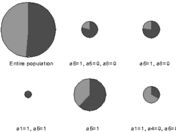
Figure 7: Visualisation of 5 best subgroups

be given after transferring just a small fraction of the data to a central node for the data mining step.

6.4

Estimating Utilities with Bounded Uncertainty

This subsection describes a first experiment that illustrates some of the pre-sented ideas. Due to a lack of publicly available datasets for distributed Data Mining, synthetic data was used. As an advantage, this allows to control the different kinds of skews.

To prepare the data, a decision tree for a domain of 10 boolean attributes has been constructed at random. For each inner node the probability of the tested attribute being 1 was fixed to a value randomly drawn from

N(0.5,0.25). The same was done for the distribution of the boolean target label at the leaves. For all examples unspecified attributes were simply com-pleted by drawing truth values uniformly. The examples were distributed to 5 sites by explicitly assigning a separate γ- and -skew to each leaf for each site. The skew-parameters were selected uniformly within the previously used intervals: γ ∈[0,1.1],∈[0,0.05]. Based on this randomly constructed tree 10.000 examples were generated as an input to the following subgroup discovery experiments.

The MIDOS algorithm, part of the Kepler toolbox, was applied to

the data, in order to select 5 best subgroups according to q(1). In figure 7 these subgroups are visualised by circles. The colours reflect the conditional distributions of the target, while the sizes represent coverage. Each dot in

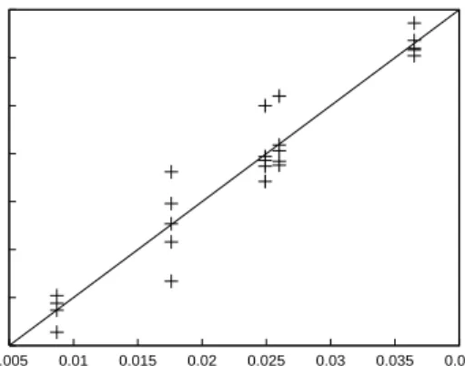
0.005 0.01 0.015 0.02 0.025 0.03 0.035 0.04 0.005 0.01 0.015 0.02 0.025 0.03 0.035 0.04 local utility global utility

Figure 8: Global vs. local evaluation.

figure 8 compares the global utility of a rule (x-axis) to the corresponding local utilities at all sites (y-axis). Dots close to the diagonal represent similar utilities, which are useful for estimating the global utilities from local ones with bounded uncertainty. Table 1 lists the bounds that could be derived based on the local estimates, exploiting γ ≤1.1 and≤0.05. It is interesting to note, that only for the largest subgroup (a5 = 1, Cov≈0.35) the bounds are useless, because for large subgroups the utility can easily be estimated from samples, instead. In contrast, the smallest of the 5 selected subgroups has aCovof below 2%. This illustrates why generating all frequent itemsets is often an inefficient approach to subgroup discovery.

Subgroup global q(1) Lower b. Upper b.

a5=1, a6=0, a8=0 0.0249 0.0231 0.0292 a5=1, a8=0 0.0260 0.0235 0.0316 a1=1, a5=1 0.0087 0.0083 0.0105

a5=1 0.0365 0.0191 0.0573

a1=1, a4=0, a5=0 0.0176 0.0164 0.0180

7

Conclusion

The behaviour of different rule selection metrics, their similarity for various skews and how well they may be estimated from samples has been investi-gated in the recent years. What is lacking is an investigation of how these metrics behave in the scope of distributed learning. This paper is a first step into this direction. First of all it has been shown that the utility measures common in the literature on subgroup discovery can be applied to homo-geneously distributed data in the same way as to a single example set. If the different sites do not share a single underlying distribution generating the data, however, then even precise estimates may yield completely disjoint rulesets at all sites, none of which contains a single one of the best n rules. For the general case a tight bound for the difference between global and local rule utilities has been proven, which allows to translate local rule utilities into global ones with bounded uncertainty. For the task of discovering rules that have a higher local than global utility it has been shown that it is at least as hard as approximating the global conditional distribution of the target attribute. For a common marginal distribution one problem can be solved locally, given a solution for the other one.

The results indicate that distributed subgroup discovery is a hard prob-lem, since it requires precise estimates of both, the global marginal and the global conditional distribution. The former may e.g. be obtained by distributed variants of frequent itemset mining, the latter by means of dis-tributed boosting. As discussed there are good reasons, however, to tackle the problem by exhaustively searching the hypothesis space, applying specific pruning strategies wherever possible.

Future work will compare concrete implementations empirically, using synthetic and real-world data in combinations with different ways to dis-tribute examples.

Acknowledgements

This work was supported by the Deutsche Forschungsgemeinschaft, Collabo-rative Research Centre 475 onReduction of Complexity for Multivariate Data Structures.

References

[1] R. Agrawal and R. Srikant. Fast algorithms for mining association rules in

large data bases. InProceedings of the 20th International Conference on Very

Large Data Bases (VLDB ‘94), pages 478–499, Santiago, Chile, sep 1994. [2] D. W.-L. Cheung and Y. Xiao. Effect of Data Skewness in Parallel Mining of

Association Rules. In Pacific-Asia Conference on Knowledge Discovery and

Data Mining, pages 48–60, 1998.

[3] P. A. Flach. The Geometry of ROC Space: Understanding Machine Learning

Metrics through ROC Isometrics. In Proceedings of the 20th International

Conference on Machine Learning (ICML-03). Morgen Kaufman, 2003.

[4] J. F¨urnkranz and P. Flach. ROC ’n’ Rule Learning – Towards a Better

Understanding of Covering Algorithms.Machine Learning, 58(1):39–77, 2005.

[5] J. F¨urnkranz and P. A. Flach. An Analysis of Rule Evaluation Metrics.

In Proceedings of the 20th International Conference on Machine Learning

(ICML-03). Morgen Kaufman, 2003.

[6] W. Kl¨osgen. Explora: A Multipattern and Multistrategy Discovery

Assis-tant. In U. M. Fayyad, G. Piatetsky-Shapiro, P. Smyth, and R. Uthurusamy,

editors,Advances in Knowledge Discovery and Data Mining, chapter 3, pages

249–272. AAAI Press/The MIT Press, Menlo Park, California, 1996.

[7] A. Lazarevic and Z. Obradovic. Boosting algorithms for parallel and

dis-tributed learning. Distributed and Parallel Databases Journal, 11(2):203–229,

2002.

[8] R. E. Schapire and Y. Singer. Improved Boosting Using Confidence-rated

Predictions. Machine Learning, 37(3):297–336, 1999.

[9] T. Scheffer and S. Wrobel. Finding the Most Interesting Patterns in a

Database Quickly by Using Sequential Sampling. Journal of Machine

Learn-ing Research, 3:833–862, 2002.

[10] S. Wrobel. An Algorithm for Multi–relational Discovery of Subgroups. In

J. Komorowski and J. Zytkow, editors,Principles of Data Mining and

Knowl-edge Discovery: First European Symposium (PKDD 97), pages 78–87, Berlin, New York, 1997. Springer.

[11] M. J. Zaki. Parallel and Distributed Association Mining: A Survey. IEEE

Concurrency, 7(4):14–25, /1999.

[12] S. Zhang, C. Zhang, and J. Yu. An Efficient Strategy for Mining Exceptions