Evaluation of different machine learning methods for MEG- based brain-function decoder

(1)

Instructor

Evaluation of different machine learning methods for

MEG-based brain-function decoder

Dennis Noordsij

Helsinki August 28, 2015 UNIVERSITY OF HELSINKI Department of Computer Science

(2)

Faculty of Science Department of Computer Science Dennis Noordsij

Evaluation of different machine learning methods for MEG-based brain-function decoder Computer Science

Master of Science August 28, 2015 59 pages + 0 appendices

classification, MEG, feature reduction, regression

Application of machine learning methods for the analysis of functional neuroimaging signals, or "brain-function decoding", is a highly interesting approach for better understanding of human brain functions. Recently, Kauppi et al. presented a brain-function decoder based on a novel feature extraction approach using spectral LDA, which allows both high classification accuracy (the authors used sparse logistic regression) and novel neuroscientific interpretation of the MEG signals. In this thesis we evaluate the performance of their brain-function decoder with additional classification and input feature scaling methods, providing possible additional options for their spectrospatial decoding toolbox SpeDeBox. We find the performance of their brain-function decoder to validate the potential of high frequency rhythmic neural activity analysis, and find that the logistic regression classifier provides the highest classification accuracy when compared to the other methods. We did not find additional benefits in applying prior input feature scaling or reduction methods.

ACM Computing Classification System (CCS):

I.5.2 Design Methodology: Classifier design and evaluation I.5.2 Design Methodology: Feature evaluation and selection I.5.4 Applications: Signal processing

Tekijä — Författare — Author

Työn nimi — Arbetets titel — Title

Oppiaine — Läroämne — Subject

Työn laji — Arbetets art — Level Aika — Datum — Month and year Sivumäärä — Sidoantal — Number of pages

Tiivistelmä — Referat — Abstract

Avainsanat — Nyckelord — Keywords

Säilytyspaikka — Förvaringsställe — Where deposited

(3)

1 Introduction

Early records of research into brain function analysis and neural pattern recognition go back to at least the 19th century, with the common example of Paul Broca’s research involving patients who suffered unfortunate traumatic brain injuries result-ing in odd behavioral effects [DPIC07]. In the 20th century, less invasive, safer, as well as better imaging modalities became available, which, coupled with advances in statistical methods lead to further understanding of brain function [DaV10]. As an example, since the introduction of functional magnetic resonance imaging (fMRI) in 1992, it has featured in well over 12.000 published papers already [Rai09] [PMB09] Nowadays machine learning is widely applied in the field of functional neuroimaging to analyze signals such as fMRI, EEG and MEG (see section 2 for a brief overview of these modalities). One such application is the design of brain-function decoding methods, where different types of stimuli or tasks can be inferred (predicted) based on the analysis of neuroimaging signals [KPHH12]. Most brain-function decoding studies so far have been based on fMRI [PMB09]; fMRI however is limited by its relatively low temporal resolution, making it an unsuitable modality for exploring the analysis of fine spectral and temporal signatures of particular brain states. For example, we know that high frequency oscillatory synchronized (electrical) activity in the brain can be associated with different brain states [Sin93]. Neuroimaging modalities capable of capturing at high temporal resolution are for example EEG and MEG [HKS10].

In 2012 Kauppi, Parkkonen, Hari and Hyvärinen published a novel brain-function decoding method that combines a feature extraction scheme utilizing spectrospatial information of neural activity captured with MEG with a sparse logistic regression method [KPHH12]. Earlier research had shown that the efficient feature selection provided by the regularized logistic regression model used is crucial for data where the feature count is (much) higher than the sample count [HKT13], as tends to be the case with neuroimaging data.

In this thesis, we take the data processed by this brain-function decoder and perform the final classification step using eight different classification methods, in combina-tion with four input scaling methods, as shown in figure 1. We hope to replicate the (good) results of the original decoder implementation, published as SpeDeBox1_{, as a}

validation of their "Spectral LDA" decoder, as well as see how these results compare

(6)

to other, both simple and sophisticated, classification methods, further outlined in section 3.4. Additionally we evaluate the effectiveness of different feature reduction methods prior to classification outlined in section 3.1.

(7)

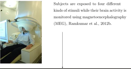
Subjects are exposed to four different kinds of stimuli while their brain activity is monitored using magnetoencephalography (MEG), Ramkumar et al., 2012b.

MEG data is used by Kauppi et al. [KPHH12] to evaluate their brain-function decoder. The method used is called spectral linear discriminant analysis (Spectral LDA), and its source code has been published as part of the Spectral decoding toolbox (SpeDeBoxa). Briefly, using patterns in rhythmic neural activity as markers for different brain states corresponding to processing the four distinct stimuli from the experiment.

a_{http://www.cs.helsinki.fi/group/neuroinf/code/spedebox/}

The authors evaluate the processed data using a logistic regression based classifier, based on previous good experience with this method [HKT13].

We take the same processed MEG data and train and classify this data using eight classification methods (including logistic regression) using four different initial scaling methods. Additionally we evaluate the effects of applying feature reduction before classification. The goal is to better validate the classification pipeline of the original decoder, as well as to suggest possible useful machine learning methods for inclusion in SpeDeBox.

Figure 1: The work done in this thesis and its relation to the work of Kauppi et al. The experimental setup is described in section 4.1. The processing pipeline of the spectral LDA decoder (first yellow box) is be described in more detail in section 4.2. Our work (green box) is described in section 4.3 with our results shown in section 5.

(8)

2 Functional neuroimaging

A typical neuroimaging experiment consists of observing neural activity (brain activ-ity) under specific conditions, such as the subject performing certain tasks or being exposed to certain stimuli [LBDM11]. A typical goal of such an experiment is to increase our understanding of the workings of the brain in general, and to find (prac-tical) applications for this new knowledge. For obvious reasons such experiments are best done using non-invasive and safe procedures.

We can roughly separate the imaging modalities, i.e. the method by which we observe or infer particular brain activity, between those which observe direct physi-ological effects of the neural activity (for example changes in blood pressure, blood flow, oxygen or glucose levels in the blood, temperature, swelling/pulsating, and so on), referred to as the hemodynamic response, and those which observe the indirect effects of the neural activity, such as in the form of electromagnetic activity [Sav01].

2.1 Hemodynamic response

A popular neuroimaging modality exploiting the hemodynamic response is func-tional magnetic resonance imaging (fMRI) [PMB09]. fMRI exploits the blood oxy-gen level dependent (BOLD) effect [Sav01]. When brain activity increases, blood flow is increased to supply (among other things) more oxygen to the active areas. This changes the relative levels of oxygenated and deoxygenated blood around the active areas, which are dia- and paramagnetic, respectively, and can be detected using fMRI [PMB09].

An inherent limitation of the hemodynamic response, and thus also of fMRI, tends to be a relatively low temporal resolution, because of the relatively slow rate of observable changes [Sav01] [Rai98]. It takes time for blood flow to increase, for tissue to move, for temperature to change, and so on, in response to a stimulus. In addition, the sensor reaction or readout times may be a limiting factor.

Spatial resolution however tends to be relatively high. fMRI, for example, can image a complete brain volume in voxels measured in cubic millimeters [HKS10]. It is expected that spatial resolution will be ultimately bound by practical limitations of the imaging modality (noise, heat, undesirable effects of large magnetic fields, and so on) rather than by physiological limitations [Sav01].

(9)

2.2 Electromagnetic response

Firing neurons inside the brain produce tiny current flows, which in turn generate tiny magnetic fields. When large enough areas fire more or less together, the sum of their effects can be measured at some distance away from the brain [Sav01]. Electroencephalography (EEG) measures the electrical effects; magnetoencephalog-raphy (MEG) measures the magnetic effects. There are a number of similarities between the two: both methods use tens to hundreds of channels (different observa-tion points), both methods can detect brain activity to a depth of about 4cm, both methods are able to sample at very high (kilohertz range and higher) rates providing excellent temporal resolution that is limited only by the neural response itself, and both methods have, at this point, a spatial accuracy of about 1cm [Sav01] [HKS10]. Both methods also share the weakness of poor three-dimensional spatial localization. Volumetric localization inside the head, i.e. determining the source of a signal, must be done using only data recorded from outside the head; this is a mathematically ill-posed problem, also referred to as the inverse problem [Sav01].

There are also a number of interesting differences between both methods.

2.2.1 Electroencephalography

In EEG electrodes are placed in a grid pattern across the scalp, making contact with the skin. The residual conductivity of electrical brain activity results in small voltage differentials between the different electrode locations. A single electrode is designated as the reference channel (cf. an electric ground, or one pole of a battery), and the voltage differentials to the other electrodes are measured [PSGS05] [Sav01]. The required equipment is, by today’s standards, cheap and uncomplicated. Spe-cial electrode "hats" exist (a kind of netting) to make electrode attachment less cumbersome (the electrodes should be placed at more or less identical locations for each session, if the results are to be compared or correlated to each other). Because the electrodes are attached directly to the scalp, subject movement does not affect readings, which simplifies post-processing (cleanup) requirements.

EEG has however two major weaknesses. Firstly there is the requirement of the ref-erence channel. There does not exist a stable refref-erence point (cf. electrical ground), so the reference channel is also an active channel, affecting all measurements with its own fluctuations. Secondly the conductivity depends on the conducting medium,

(10)

i.e. is affected by the shape and density of the various tissues, particularly the skull, which means signals are attenuated according to individual and local physiology.

2.2.2 Magnetoencephalography (MEG)

In MEG highly sensitive gradio/magnetometers are positioned in a grid pattern sur-rounding the scalp in order to pick up extremely small (tens of femtotesla) magnetic fields [HKS10]. Because these field strengths lie below the normal ambient back-ground noise a shielded environment and highly sensitive superconducting quantum interference devices (SQUIDs) are needed. MEG therefore requires expensive and wieldy experimental setups, such as shown in figure 2.

Physical contact with the scalp is not needed, this however also means that the sub-ject will likely move with respect to the sensor array, complicating post-processing as the measured intensity of the magnetic fields depends on the distance between the (moving) source and the (fixed) sensors. Algorithms that sufficiently compen-sate for (among other things) subject motion [TaK05] [TSK05] have however been developed and have greatly improved the usefulness of MEG.

MEG does not need a reference channel like EEG, and the magnetic fields are not affected by physiological variations. Furthermore there is one more important difference to EEG. The orientation of the magnetic fields depends on the physical orientation of the corresponding current flow, i.e. the orientation of the neurons. Radially oriented fields are not seen by MEG, only tangentially oriented fields. This means MEG sees "less" of the same brain activity than EEG. Generally, due to brain physiology, signals originating from deep inside the brain tend to be more radially oriented (less visible), whereas signals originating from the outer areas of the brain are more tangentially oriented (more visible). One can argue this to be an advantage or a disadvantage over EEG; in practice it has not deterred applications of MEG [HKS10].

Additional imaging variants include combining EEG and MEG, or even EEG, MEG and fMRI [HHP05].

(11)

Figure 2: MEG recording setup example. Image credit: National Institute of Mental Health (NIMH).

(12)

3 Classification

Fundamentally what we mean by classifying is assigning or inferring a particular label to a particular set of observations, or properties [HTF09]. For example, we can tell apart different types of fruits by their physical appearance, which is made up of their color, size, shape, but also by their taste, texture, or background information such as the type of plant they grow on, the time of year they bloom, and what the ideal growing conditions are. Of course, at some point we have had to learn the properties of these different types of fruits.

In this thesis we attempt to classify (label) neuroimaging data. By looking at recorded data, we try to infer (guess, or predict) what kind of stimulus the brain was processing at that particular moment. To do this we first look at examples; we look at recorded data where we know there was a visual stimulus, at recorded data where we know there was an auditory stimulus, and so on. Afterwards, we use this knowledge to try and assign a label to unlabeled recording data. This process is a form of supervised learning [Bis06].

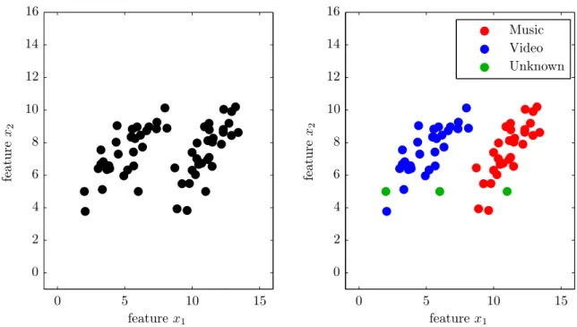
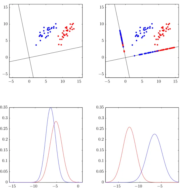
Unsupervised learning would be looking at unlabeled data, and trying to find dif-ferent classes. A simple example would be giving a bucket filled with apples and bananas to someone who does not know what apples or bananas are, and asking them to sort the bucket by what they would assume to be different types of fruit. Consider the left plot in figure 3, as the result of a neuroimaging experiment where we recorded 2 channels of data, shown in the x-axis and y-axis. Based on visual inspection, we would probably conclude we observed two distinct brain states. This is a form of unsupervised learning, as we do not know the actual exact answer. But consider the right plot, where we recorded data under controlled conditions where we labeled each recording sample with the corresponding stimulus. We can now try and learn (model) the particular features of both brain states. Using this model, we can take unknown samples (shown in green), and assign them to a particular class based on their properties. I.e., by looking at a particular reading we try to predict if the subject was listening to music, or watching a video, at the time of recording. We refer to a classifier as a particular combination of input processing, modelling, and predicting methods [DHS06]. For example, one classifier may work by learning statistical properties of the different classes, whereas another classifier may compare unknown samples directly to the known samples to try and find its closest match. A trained classifier thus maps inputs (in our case high dimensional neuroimaging

(13)

Unknown Video Music fe a t u r e x2 feature x₁ fe a t u r e x2 feature x₁ 0 5 10 15 0 5 10 15 0 2 4 6 8 10 12 14 16 0 2 4 6 8 10 12 14 16

Figure 3: Both plots contain the same data points. On the left, we do not have any class information, and we can use unsupervised learning to deduce that there are probably two different states (classes), as well as learn the properties which allow us to assign future samples to either of the classes. Of course, this is highly ideal data, from real world data it can be difficult to deduce how many different classes there are. In the right plot we do have class labels, i.e. we do know to which activity each sample belongs. Based on this class information, we can try to assign a class label to future (unknown) samples. Approaches can vary from using statistical properties, to simply looking for the known sample which most closely mirrors the unknown sample.

(14)

data) to outputs (in our case one of four class labels).

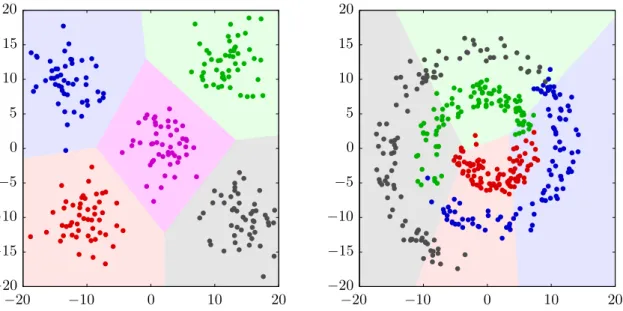
Consider figure 4. A classifier, in this case a minimum distance classifier (see section 3.4.1) was trained on the colored samples shown, on the left with five classes, and on the right with four classes. For each of the possible observations of input data (two dimensional in this case, the x-axis and y-axis) the corresponding mapping to its class label is shown as the background color. This particular classifier creates linear decision boundaries, but we will also introduce some non-linear classifiers. A classifier may also project its input data, for example a classifier could attempt to "unroll" the spiral data on the right, which would result in a stacked bar that can be linearly separated. The difficulty is of course in knowing when and how to do this, i.e., determining the distribution of the input data.

Note that we assume the data has been appropriately pre-processed; real world data can come with noise, random outliers, missing values, and so on. A first step is to clean up this data, which in our case has been done as part of the brain-function decoder, the yellow blocks in figure 1, further described in section 4.2.

3.1 Feature reduction

Consider the right plot of figure 3. In the end our goal is to distinguish between the different classes, in this case "Music" and "Video". Do we need all of the data to do this? Do we need to preserve the exact structure, or can we simplify the data by discarding information which does not aid in separation of the classes? A reason we may want to ask this is that as a general rule, more data means more complexity, which means more processing requirements. If we have very large datasets with very high dimensionality, it may be a good idea to try and reduce this data volume, insofar as it does not (significantly) affect what we ultimately care about: separability (class discrimination).

Consider an example of learning to distinguish between cats and dogs. Suppose we list as many properties as we can, in order to maximize our chances of correctly classifying future observations. We may end up with the "number of legs", as well as "number of paws". Of course, these are redundant, as they correlate perfectly. We can then discard either of them, or, choose to keep one of them. This is feature reduction by feature selection. (Additionally, both cats and dogs tend to have four legs, so this property can be discarded entirely as it does not help us to distinguish between cats and dogs).

(15)

−20 −10 0 10 20 −20 −10 0 10 20 −20 −15 −10 −5 0 5 10 15 20 −20 −15 −10 −5 0 5 10 15 20

Figure 4: Decision boundaries as found by the minimum distance classifier. This classifier is further described in section 3.4.1, but it basically looks at how far a sample is removed from the means of the different classes’ samples. The shaded areas indicate how any sample inside those areas would be classified. As this is a linear classifier (linear decision boundaries), it is unable to partition the spiral data adequately.

Another possibility is to combine features. For example, we may derive a body mass index (BMI) from height and weight properties. If this BMI is -for the purpose of separating between the classes- just as useful as having height and weight separately, we can replace those two features with a single new feature. This is feature reduction by feature extraction.

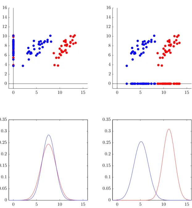
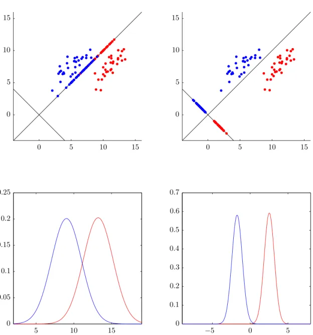
In figure 5 we apply feature reduction by projecting the data onto the y- and x-axis, thereby reducing the data from two-dimensional to one-dimensional. The bottom row shows the prevalence of the different classes on their new single axis. Here we can see that by projecting onto the x-axis we maintain separability; if we would project the three green samples from figure 3 onto the x-axis as well we would still be able to confidently classify them.

The choice of projecting onto the y- or x-axis is of course arbitrary. We can project any way we want, such as for example in figure 6. It would appear from visual inspection that these projections are inferior to an x-axis projection, because there is a small section where both classes are represented, and where we are thus unable to confidently assign a sample to either class.

(16)

0 5 10 15 0 5 10 15 0 5 10 15 0 5 10 15 0 0 .05 0 .1 0 .15 0 .2 0 .25 0 .3 0 .35 0 0 .05 0 .1 0 .15 0 .2 0 .25 0 .3 0 .35 0 2 4 6 8 10 12 14 16 0 2 4 6 8 10 12 14 16

Figure 5: Top row: projecting the data in figure 3 onto the y- and x-axis. Bottom row: the distribution of the samples after projection. For good separability we want distinct peaks and as little overlap as possible. If we project onto they-axis, we lose all class discrimination information. If we project onto the x axis, we hardly lose any separability when compared to the two-dimensional data before the projection.

(17)

−15 −10 −5 −15 −10 −5 0 −5 0 5 10 15 −5 0 5 10 15 0 0 .05 0 .1 0 .15 0 .2 0 .25 0 .3 0 .35 0 0 .05 0 .1 0 .15 0 .2 0 .25 0 .3 0 .35 −5 0 5 10 15 −5 0 5 10 15

Figure 6: Similar to figure 5, but now projecting onto two arbitrary vectors. We can see in the bottom figures that both projections provide better separability than projecting onto the y-axis, but less than projecting onto the x-axis.

(18)

In the first case, projecting onto the x- and y-axis, we are performing feature re-duction through feature selection: we choose one feature (x or y), and completely discard the other (y orx). In the second case, we are using both x and y values to calculate a new single feature, here we perform feature reduction through feature extraction.

These differences lead to a question: can we find out the optimal projection (optimal in the sense of maximizing class discrimination or separability)?

3.1.1 Principal component analysis (PCA)

In figure 7 we perform principal component analysis (PCA). PCA is a method of finding the orthogonal projection vectors which project the data in a way which fits as much variance into as few principal components as possible, yielding an ordered set of principal components where each component contains less variance than the previous component, with as much variance in a single component as possible [Bis06] [DHS06]. We can use this for feature reduction by taking only those vectors with the highest variance, and discarding those with the lowest, using any thresholding we choose, for example by choosing a specific number of principal components, or choosing those principal components which contain a certain amount of the total variance. In this example in figure 7, we can see that the two vectors are aligned with the data clouds, such that on the left the variance is maximized, and on the right it is minimized.

However, our ultimate goal is separating the different classes. If we would imagine one of the data clouds to be rotated by 90 degrees, then a projection which would maximize the variance for one of the classes would minimize the variance of the other. It is also not the case that components with higher variance are necessarily more important or useful for regression than components with smaller variances [Jol82] [BHPT06].

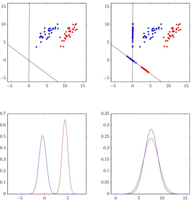
3.1.2 Linear discriminant analysis (LDA)

Another possibly useful feature reduction method is linear discriminant analysis (LDA), a method published already in 1936 [Fis36], its application shown in figure 8. Unlike PCA, LDA’s objective is to maximize class separability (class discrimination). It produces one linear function for each class, with each sample belonging to the class whose linear function returns the highest value [DHS06]. When the dimensionality

(19)

−5 0 5 5 10 15 0 5 10 15 0 5 10 15 0 0 .1 0 .2 0 .3 0 .4 0 .5 0 .6 0 .7 0 0 .05 0 .1 0 .15 0 .2 0 .25 0 5 10 15 0 5 10 15

Figure 7: PCA projecting the data from figure 3. PCA optimizes for preservation of maximum variance. The variance in this figure is represented by the surface area under the curves in the bottom row. Note especially that separability means we want to have as little overlap between the curves as possible, but it is not important how much surface area the curves have. Particularly: the right plot has better separability than the left, despite preserving the least variance.

(20)

0 5 10 15 −5 0 5 −5 0 5 10 15 −5 0 5 10 15 0 0 .05 0 .1 0 .15 0 .2 0 .25 0 .3 0 .35 0 0 .1 0 .2 0 .3 0 .4 0 .5 0 .6 0 .7 −5 0 5 10 15 −5 0 5 10 15

Figure 8: LDA projecting the data from figure 3. On the left: maximum separability (minimum overlap). On the right, minimum separability (complete overlap).

(21)

is higher than the number of classes, this automatically results in feature reduction. However, high dimensional data with relative low sample counts (as is the case with our MEG data) is a bad fit for LDA. Consider having 2 points in a 2-dimensional space: one can always find a separating hyperplane. Now consider 100 points in 256-dimensional space: again, one can again always find a separating hyperplane. However, these hyperplanes are most likely to just fit the training data, and not to generalize to the true data model or distribution. This effect is demonstrated in figure 9. Section 5.3 shows this effect to apply also to our tested MEG data, resulting in poor classification accuracies.

3.1.3 Independent component analysis (ICA)

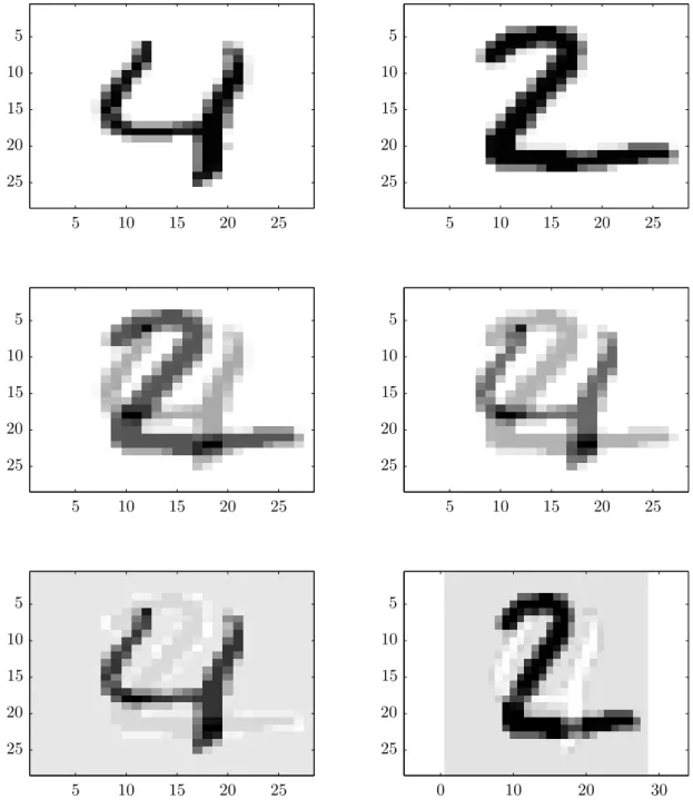
Independent component analysis (ICA) is an unsupervised, blind source separating (BSS) feature extraction method which works by minimizing statistical dependence [HKO01]. When there are n sources generating a signal (example: people in a room speaking simultaneously), and there are least n linear combinations of these signals observed (example: microphones located throughout the room), ICA is able to, under certain assumptions, separate the originaln sources. Because one of these is an assumption of non-Gaussianity, we use a different example than figure 3 to illustrate the effect. Figure 10 shows linearly combining two separate digits from the well-known [Bis06, p.2] [HTF09, p.4] MNIST dataset, and then separating their sums into the original digits.

However, because ICA is unsupervised it has no knowledge of the class labels, and there is no guarantee that the original sources provide as much class discrimination as the original (mixed) sources. This can be seen in the results in section 5.3. Supervised variants of ICA have been created, specifically for classification purposes [KCC01] [BrV05] [SYK01], but have not been considered in this thesis.

3.2 Scaling

Depending on the classifier method and its particular implementation, results may be improved by standardizing the input data. Typically this means scaling to unit variance, and shifting to zero mean. Additionally some classification methods may have standardization built-in, or as an option. We have used four different scaling methods, listed in section 5, page 42.

(22)

−0.4 −0.2 0 0.2 0.4 −0.3 −0.2 −0.1 0 0.1 0.2 −0.2 −0.1 0 0.1 0.2 −0.2 −0.1 0 0.1 0.2 −0.2 −0.15 −0.1 −0.05 0 0 .05 0 .1 0 .15 −0.2 −0.15 −0.1 −0.05 0 0 .05 0 .1 0 .15 0 .2 −0.3 −0.2 −0.1 0 0 .1 0 .2 −0.25 −0.2 −0.15 −0.1 −0.05 0 0 .05 0 .1 0 .15 0 .2

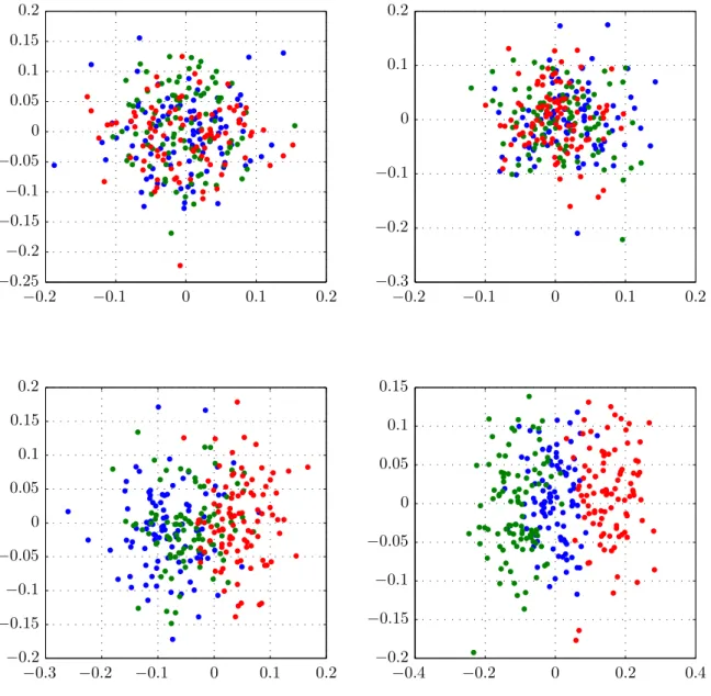
Figure 9: In each plot we show 50 samples taken from the same multivariate Gaussian distribution and assign them randomly to four different classes. We then apply LDA feature reduction. In the top-left 10-dimensional data, in the top-right 50-dimensional data, in the bottom-left 130 50-dimensional-data, and in the bottom-right 145 dimensional-data. We can see that as the dimensionality rises, the relatively low number of samples causes LDA to overtrain and amplify existing random variance to suggest separability where there is none. As the MEG data has a similarly high dimensionality relative to its sample counts, we should be cautious when applying LDA.

(23)

0 10 20 30 5 10 15 20 25 5 10 15 20 25 5 10 15 20 25 5 10 15 20 25 5 10 15 20 25 5 10 15 20 25 5 10 15 20 25 5 10 15 20 25 5 10 15 20 25 5 10 15 20 25 5 10 15 20 25

Figure 10: Top row: 2 separate digits from the MNIST dataset. Middle row: two independent linear mixes of the two digits. Bottom row: blind source separation applied in the form of ICA, recovering the individual digits.

(24)

3.3 Training, validation, and testing

After processing the input data, applying possible scaling and/or feature reduction methods, the first step in classification is training: building a model by identify-ing the characteristics of the different classes, and what sets them apart [HTF09] [DHS06]. For example, if we were to classify flowers, we may learn that certain flow-ers only come in certain colors, that some types of flowflow-ers have thorns, and grow taller than others. The more useful (varied) training samples -examples- we have, the more accurately we can build such a model.

Then, when we have completed the model, we can start to categorize (classify) unknown flowers. When we see a red flower with thorns we would therefore be quite confident that this flower is in fact a rose, and not a tulip. Of course, in this example the properties of flowers are intuitively understood. When it comes to brain state classification, we have many hundreds of features that by themselves have no particular meaning; instead, we look for statistical properties of the features that most convincingly partition the samples (the readings) by the corresponding brain state.

When we build such a model, there may be several choices that we have to make. For example, how sensitive are we to outliers? We would therefore also like to optimize our choices, i.e. the set of adjustable parameters, also called hyperparameters, which a particular classification algorithm takes as an input. A good approach to do this is to pick some initial hyperparameter values to the best of our ability (which could even mean randomly), and then iterate by retraining using different values, and observing the effects on the final classification accuracy. However, a risk with this approach is that a classifier becomes optimized for a very specific set of samples, instead of for the general model the samples come from. To prevent this, we introduce the concept of having a specific set of samples, called the validation set [DHS06], specifically for the purpose of repeatedly trying out different combinations of hyperparameter values.

Once we have determined the best choice of parameters, we then try to classify an independent set of samples to evaluate how well the classifier really works. It is important that this test set consists of samples that are as independent as possible of the training and validation samples. In our case, the test data consists of a completely independent recording session, representing more or less the ideal case. If we have a relatively low number of samples, as is the case with the MEG data,

(25)

we can also mix the samples that we have available for training and validation into several different combinations of training and validation sets, classifying all of them and taking the average accuracy. This way we smooth out the result of the hyperparameter choice, making it less susceptible to optimizing for a particular outlier or unfavorable partitioning. This approach is called cross-validation [DHS06].

3.4 Classification methods

In addition to logistic regression used by Kauppi et al. [KPHH12], we have tested seven other popular classification methods, described in the following pages, and summarized on page 42.

3.4.1 Minimum distance classification

A minimum distance classifier (also called a centroid classifier) is a very straight-forward and intuitive method of classification, which works well when the data is clustered in data clouds such as in the left side of our example in figure 3 [DHS06]. For each of the classes the center value (centroid) is calculated, and each point is classified according to the centroid it is closest to. Note in particular that the variance of a given class distribution is ignored. The decision boundaries of the minimum distance classifier were shown in figure 4.

3.4.2 k-Nearest neighbor classification

The k-nearest-neighbor classifier works by treating the training data as a corpus of lookup data, or reference samples [DHS06]. Classification is then performed by finding thekmost similar reference samples to a test sample, and choosing the most likely class label, typically based on plurality. This classifier makes no assumptions about the particular distribution, or shape, of the class data, and can function very well when there is enough separation between samples of different classes compared to the distances between samples of the same class. This is demonstrated in figure 11, which also shows the effect of various choices ofk. Several optimizations exist to speed up the search for neighbors or provide indexing methods [AMNSW98] [BKL06] [HASZ11].

(26)

3.4.3 Naive Bayes classification

Consider the artificial data in figure 12. For each sample we wish to classify, we can ask, for each class C, the question "what is the probability that a random sample drawn from the underlying distribution belonging to class C would be this exact sample?". The particular class C for which this probability is highest is then assigned to this sample.

Of course, this requires one to know, or to be able to fairly accurately model, the underlying distribution of each class. Suppose we assume the class distributions are normal distributions with a mean and variance that can be learned from the known samples.

Let x be an unknown sample having features f1, f2, ..., fn. Let c be the class label

belonging to x, which c∈C be class labeli. Then:

p(c=Ci|x) = p(c=Ci|f1, ..., fn)

Using the Bayes Theorem (Bayes Rule), [DHS06, p. 614] this can be written as:

p(c=Ci|x) =

p(c=Ci)p(f1, ..., fn|c=Ci) p(f1, ..., fn)

where p(Ci) is the prior probability of any given sample belonging to this distribu-tion. In our example case the probability for each of n classes is 1_n.

We want to find for which i this probability is highest (i.e.: which distribution is the mostly likely to have produced this particular sample).

We can simplify by ignoring the denominator, as the value of f1, ..., fn does not change, i.e.:

p(c=Ci|x)∝p(c=Ci)p(f1, ...fn|c=Ci)

This becomes:

p(c=Ci|x)∝p(c=Ci)p(f1|c=Ci)p(f2|c=Ci, f1)...p(fn|c=Ci, f1, f2, ..., fn−1)

which however becomes computationally more challenging asn (the number of fea-tures) gets larger.

(27)

A surprisingly effective [Ris05] simplification is to assume conditional independence, that is, for any i and j, to assume that the value of fi is independent of the value

of fj, i.e. for n possible classes and m features:

Because of this naive assumption (of conditional independence) this method is com-monly known as the naive Bayes classifier. The decision boundaries for the naive Bayes classifier are shown in figure 12.

3.4.4 Linear SVM classification

Support vector machines (SVM) attempt to find the optimal separating hyperplane separating two classes, maximizing the distance to the closest point from either class [DHS06] [HTF09], see the top-left plot in figure 13

A hyperplane can be written as the set of points xsuch that

w·x−b= 0

where w is the normal vector of the hyperplane, and _||_wb_|| is the offset of the hyper-plane alongw.

As can be seen in the top-left plot in figure 13, there will exist two (in this 2-dimensional example) margin hyperplanes, the dotted lines, which fully separate the two classes. It follows that these intersect some of the datapoints (if not, then either the margin could be moved further away and still separate the classes, or the margin would not be separating in the first place, which contradicts the initial assumption), these select datapoints are called the support vectors, and are circled in green. It is these support vectors that define the SVM model. Classification is done by checking on which side of the hyperplane datapoints fall, i.e. smaller or larger than 0 (in the unlikely case that the result is exactly 0 the outcome can be assigned randomly).

(28)

Lying on either side of the hyperplane, these margin planes can be conveniently defined as:

w·x−b= 1

and

w·x−b=−1

All xi of the first class must then give a result ≥ 1, and all xi of the second class

must give a result ≤ −1. Letting yi be the class label as well as functioning as the

sign (by using classes −1 and 1), and n the number of training samples, this gives the following function:

yi(w·xi−b)≥1

It then becomes an optimization problem to findw and b such that the margin _||_w2_|| is maximized [HTF09].

While adaptions of the SVM method have been made to enable multiclass classifica-tion [HsL02] [LLW04], the original binary SVM classifier can be used by decomposing the multiclass classification task into a set of binary classification tasks. Two com-mon approaches are one-versus-all classification (where each class is separated from the combination of the remaining classes) and one-versus-one classification (where each class is separated from each other class individually). The results of these binary classifications can be combined via voting, or a technique based on error correcting codes [DiB94]. The results here are obtained using libsvm [ChL11] are based on one-versus-one classification.

The decision boundaries of the linear SVM classifier are shown in figure 13, show-ing the effect of the choice of the cost factor (the slack factor) in the left plots. In the bottom-left, the decision boundaries are perfectly symmetrical between the outermost samples of the neighboring classes, whereas in the top-left the decision boundaries have significant slack in them and ignore the positions of the outermost samples of the neighboring classes.

The decision boundaries for the linear SVM classifier are shown in figure 14.

3.4.5 Non-linear (RBF kernel) SVM classification

A non-linear variant of SVM classification works by applying a kernel function to transform the data to some other, possibly higher-dimensional, space, and to do so while still allowing efficient optimization [HTF09]. The resulting separating hyper-plane can then be non-linear in the original input space. A common approach is to

(29)

apply to a radial basis function (RBF) kernel [ChL11]. Figure 15 illustrates the type of decision boundaries produced by SVM when applying a RBF kernel. Using an RBF kernel variant of SVM requires optimizing two hyperparameters. Other kernel variants (polynomial, etc.) exist, but require more hyperparameters that need to be optimized, and will not be considered here.

3.4.6 Multilayer perceptron classification

An artificial neural network can be considered as a processing unit with a number of input and output nodes [DHS06], see for example figure 16. Depending on the levels of the input signals, particular output signals are produced, similar to an electric circuit.

A neural network consists of an input layer with n inputs, an output layer with m

outputs, andk hidden layers, each of which can have any number of nk nodes itself.

Nodes are connected "left-to-right", i.e. all nodes in the input layer are connected to all nodes in the next layer, and so on, until the final output layer.

Each node has a transfer function, typically linear or sigmoidal, whose parameters are automatically optimized during classifier training. The node produces a partic-ular output based on its input value (in the case of the input layer this is the input value directly, otherwise it is the sum of all the inputs of that node). Nodes therefore threshold or transform their input signals. Because each node is affected by all of its inputs, complex transformations are possible. This is illustrated in figure 17. Training a neural network consists of providing the input values, or features, together with the desired output values, and having the node parameters iteratively evolve to produce (close to) the desired outputs by altering their transfer function properties in a feedback loop.

For our data we have 256 input features. These 256 input features should be mapped to network outputs describing class labels. There are different ways in which we can encode the output. We can have a single output, and have class label 1 produce a value of 0, class label 2 a value of 0.33, and so on. For better accuracy however we specify 4 outputs, representing the 4 output classes. This way the output value for each class is produced separately. For each class label, the corresponding output signal is 1, the other signals are 0. The classification result is then simply found by comparing the confidence (probability) of the input belonging to each of the four possible classes.

(30)

Figure 18 shows the classification boundaries for a multilayer perceptron classifier.

3.4.7 Random forest classification

Consider the left plot of figure 19, and the optimal linear decision boundary as determined by the SVM classifier in figure 13. All datapoints falling to the right (the red side) of the decision boundary are convincingly classified as red, however some of the datapoints falling to the left (the blue side) will be classified wrong. We can split this classification problem by subtracting the red "half" and applying a new classifier to the remaining left side, and repeat this procedure until all leafs of the resulting classification tree provide definitive classification outcomes. The result will be a binary decision tree. Each node in a decision tree consists of some predicate p (in itself a classifier) which performs a test on a localized part of the data, and emits a true or false result, sending classification down the left or right branch respectively. In each branch the remaining data window is reduced, leading to a finite tree depth and eventual convergence on a classification result.

The right plot of figure 19 shows the decision boundaries created by an exhaustive decision tree (the choice of partitioning on thexvalue is an arbitrary implementation detail of the demonstrated example, a decision tree is free to use any predicate which somehow separates its partition further). Everything falling on the right side of the middle boundary is classified as red, everything on the left is classified as blue, except when falling exactly between the two boundaries on the left, then the sample is red again.

We notice from figure 19 that while the decision boundaries fully classify the training data correctly, the resulting classifier probably does not generalize well. Outliers are unlikely to be restricted to the exact narrow band based only on the xfeature. We also notice that the two red outliers are only outliers when considering thexfeature, not when considering theyfeature. While this particular example is unfortunate, as the data loses separability when projected onto theyaxis, it raises the possibility of employing multiple decision trees restricted to different subsets of the feature space, and classifying according to the plurality of their outcomes.

Classifiers employing such a set of decision trees, trained on random selections of the feature space, are called random forests [PBN11], or random forest classifiers (other methods involving multiple decision trees may also speak of bags of trees). Employing multiple decision trees reduces overtraining; while outliers may end up as

(31)

single leafs it is unlikely to affect classification in general, as the likelihood of such an exact sample occurring in the test data is small when considering the real domain. Pruning decision trees, and employing heuristics such as not allowing a new leaf to be created unless more than some k samples are affected (a smoothening effect), are used less to improve classification, and more to reduce storage requirements and tree complexity.

Random forest based algorithms and classifiers are especially popular in computer vision applications [PBN11] [DFPLR12] [SSKFFBCM13]. RF based classification of our sample data is shown in figure 20. This classifier performs well with minimal hyperparameter tuning efforts.

3.4.8 Logistic regression

Logistic regression is a form of regression suitable for binary dependent variables, that is, an output being exactly 0 or 1, instead of being continuous. For each of the four class labels we use logistic regression to give us a probability for a particular datapoint belonging to that class. We then choose the class label with the highest probability as the classification result, similar to how we encode the outputs of a neural network with four output nodes.

The difference to linear regression can be nicely explained visually. Consider the datacloud on the left in figure 21, we can find an optimal predictor function with least-squares regression. Note that the dependent variable here is continuous. Now consider the binary data on the right, and assume it expresses whether a particular datapoint belongs to some class, by having the value be1or0respectively. Here such a linear regressor does not make sense, because we want the result to be bounded between 0and 1.

Logistic regression solves this problem by making the dependent variable the log of the odds ratio:

ln p 1−p

which is called the logit. The regression equation then gives us this logit, which is then converted to a probability using:

p= e

logit 1 +elogit

(32)

This then gives the nicely bounded transition between 0 and 1 seen on the right in figure 21.

The classifier we use is glmnet [FHT10], which uses a multinomial variant to give us the four class probabilities per sample, and which uses elastic net regularization [ZoH05].

Figure 22 shows the classification boundaries for the glmnet classifier for our sample data.

(33)

−20 −10 0 10 20 −20 −10 0 10 20 −20 −10 0 10 20 −20 −10 0 10 20 −20 −10 0 10 20 −20 −10 0 10 20 −20 −10 0 10 20 −20 −10 0 10 20 −20 −10 0 10 20 −20 −10 0 10 20 −20 −10 0 10 20 −20 −10 0 10 20

Figure 11: Decision boundaries as found by the kNN classifier. In these three rows, top-to-bottom,k was chosen as1,50, and200respectively. As can be seen,k needs to be chosen carefully to prevent both under-training and over-training. This plot suggests lower values of k would be safer than larger values, as these have the risk of classes bleeding into each other.

(34)

−20 −10 0 10 20 −20 −10 0 10 20 −20 −15 −10 −5 0 5 10 15 20 −20 −15 −10 −5 0 5 10 15 20

Figure 12: Decision boundaries as found by the naive Bayes classifier. Note the test data in the left plot is in fact normally distributed with its features conditionally independent, and thus ideal for the naive Bayes classifier. In the right plot we see that accounting for the variance provides significant improvement over a mean-only model (the minimum distance classifier in figure 4).

(35)

2 4 6 8 10 12 14 2 4 6 8 10 12 14 2 4 6 8 10 12 14 2 4 6 8 10 12 14 3 4 5 6 7 8 9 10 11 3 4 5 6 7 8 9 10 11 3 4 5 6 7 8 9 10 11 3 4 5 6 7 8 9 10 11

Figure 13: The solid line represents the decision boundary found by the linear SVM classifier; the circled datapoints represent the chosen support vectors which were used to establish the decision boundary and its margins. The top left shows the ideal case, clean separation without any outliers. The top-right shows the effect of a single outlier: the support vector is placed suboptimally. The bottom-left shows the result of introducing a slack factor (a tolerance for outliers). The bottom right shows how this outlier tolerance leads to good separation where actual linear separation would otherwise not even be possible (due to the additional red datapoint deep inside the blue area).

(36)

−20 −10 0 10 20 −20 −10 0 10 20 −20 −10 0 10 20 −20 −10 0 10 20 −20 −10 0 10 20 −20 −10 0 10 20 −20 −10 0 10 20 −20 −10 0 10 20 −20 −10 0 10 20 −20 −10 0 10 20 −20 −10 0 10 20 −20 −10 0 10 20

Figure 14: Decision boundaries as found by the linear SVM classifier for increasing tolerances to outliers (the cost parameter).

(37)

−20 −10 0 10 20 −20 −10 0 10 20 −20 −10 0 10 20 −20 −10 0 10 20 −20 −10 0 10 20 −20 −10 0 10 20 −20 −10 0 10 20 −20 −10 0 10 20 −20 −10 0 10 20 −20 −10 0 10 20 −20 −10 0 10 20 −20 −10 0 10 20

Figure 15: Decision boundaries as found by the non-linear (RBF kernel) SVM clas-sifier. The hyperparameters must be chosen to avoid overtraining (bottom row), but if chosen optimally (middle row) RBF-SVM provides good separation.

(38)

Figure 16: An artificial neural network with 256 inputs and 4 outputs. We let each output be the probability that the input sample belongs to the corresponding class, by training the neural network on for example the output1000for class1, the output

0100 for class 2, and so on. This way each output is optimized for recognizing its corresponding class. input input input

f

output

f

Layer i Layer j node ik node jk ik jk

Figure 17: All outputs from layeri−1are connected to each node in layeri. Transfer functionf_ik combines/thresholds these inputs to produce a single output. Together each output of the nodes in layeri is connected to each node in layer j, and so on.

(39)

−20 −10 0 10 20 −20 −10 0 10 20 −20 −10 0 10 20 −20 −10 0 10 20 −20 −10 0 10 20 −20 −10 0 10 20 −20 −10 0 10 20 −20 −10 0 10 20 −20 −10 0 10 20 −20 −10 0 10 20 −20 −10 0 10 20 −20 −10 0 10 20

Figure 18: Multilayer perceptron classification, from top to bottom: no hidden layers, tangent sigmoid output function (tansig), one hidden layer with five (left plot) and four (right plot) nodes, tansig output, and two hidden layers, both with five and four nodes, all tansig output functions. With no hidden layers the decision boundaries are linear and not very good in either plot. One hidden layer improves the result dramatically, but it takes two hidden layers to properly capture the proper decision boundaries in both cases, without overtraining (note the blue outlier in the spiral graph which is correctly ignored in the bottom plot).

(40)

0 5 10 15 2 4 6 8 10 12 14 3 4 5 6 7 8 9 10 11 3 4 5 6 7 8 9 10 11

Figure 19: Basic example of decision boundaries for a maximally trained decision tree. There are four horizontal partitions, corresponding to the blue, red, blue, and red classes. This is also an example of overtraining, as the individual outliers should not warrant their own partitions. A reasonable choice would have been a single decision boundary. −20 −10 0 10 20 −20 −10 0 10 20 −20 −15 −10 −5 0 5 10 15 20 −20 −15 −10 −5 0 5 10 15 20

Figure 20: Decision boundaries as found by the random forest classifier. The decision boundaries are not smooth lines or curves, but the effect of partitioning. This classifier provides decent separation for both plots, without overtraining, and needs almost no tuning. However, we can see that in sparse areas the decision boundaries are not placed as well as shown in the SVM example in figure 13.

(41)

0 2 4 6 8 10 6 8 10 12 14 − 1 −0.5 0 0 .5 1 1 .5 2 2 3 4 5 6 7 8 9 10 11 12

Figure 21: On the left continuous data showing its linear regressor; on the right binomial data for which the red regressor makes no sense. By using the log of the odds ratio as the dependent variable (i.e. using logistic regression) we get a result bounded between 0 and 1, the cyan curve.

−20 −10 0 10 20 −20 −10 0 10 20 −20 −15 −10 −5 0 5 10 15 20 −20 −15 −10 −5 0 5 10 15 20

(42)

4 Brain-function decoder design and experiments

In sections 4.1 and 4.2 we describe the MEG decoding experiment and brain-function decoder design from earlier work (Ramkumar et al., Kauppi et al.). In section 4.3 we describe how different classifiers and preprocessing options have been evaluated in this thesis.

4.1 Experimental setup

Consider figure 1. In a previous, unrelated experiment (Ramkumar et al., 2012b) MEG data was acquired for eleven subjects. Two sessions had to be discarded due to problems, leaving session data for nine subjects.

Subjects each took part in two separate 12-minute long MEG recording sessions. Both sessions can thus be considered completely independent; data from the first session is used for training and validation, and data from the second session for the final testing.

Subjects were exposed to three kinds of stimuli: auditory, visual and tactile. Lack of stimuli, i.e. moments of rest, is considered a fourth state.

Visual stimuli consisted of silent home-made video clips of either people (with a focus on their faces or hands), or buildings. Auditory stimulation consisted of specific beeps and pre-recorded speech. Tactile stimulation was applied to left and right hands simultaneously, using pneumatic diaphragms operating at 4 Hz attached to index, middle and ring fingers.

This data was then analyzed using the brain-function decoder described in the next section, after which we performed our classifier evaluation, outlined in the section after that.

4.2 Preprocessing and feature extraction

As noted in the introduction, and shown as the yellow boxes in figure 1, the brain-function decoder by Kauppi et al. [KPHH12] is based on correlating the observed rhythmic neural activity patterns to exposure to the different stimuli, built around a method called spectral LDA (SLDA).

Figure 23 shows a schematic of the high level building blocks of the brain-function decoder, on which we elaborate more below.

(43)

Figure 23: Preprocessing pipeline. 204 channels are recorded. The data is then filtered via signal space separation (SSS) to reduce artifacts and perform motion correction, after which the signals are decomposed using a short-time Fourier trans-form using 2 second windows and 50% overlap for the first session, and no overlap for the second session. 64 independent components are estimated using Fourier-ICA (fICA), by frequency band selection, outlier removal, dimension reduction, whiten-ing, and finally estimation. Spectral LDA vector projection and combining then yields 256 dimensional data.

(44)

4.2.1 Artifact removal

MEG measures the magnetic fields created by electrical brain activity. Because these levels lie below the ambient background noise, and depending on setup and shielding, these readings may be sensitive to outside magnetic field interference. An elegant method dubbed signal-space separation (SSS, [TaK05]) exploits fundamental properties of magnetic fields to decompose the recordings into signals originating from inside and outside the measuring volume (i.e. signals originating from inside the brain, and signals which have come from outside interference and are therefore noise), very effectively suppressing external interference, while reducing artifacts and providing motion correction. Signal-space separation development has been a very important development and enabler for MEG data processing.

4.2.2 Epoch extraction

The signals are then divided into two-second windows (epochs) to which a short-time Fourier transform is applied, creating a short-time-frequency decomposition for each window. In order to create more training data, epochs from the first session were created with a 50% overlap; this was not done for the second session (to be used as test data) so as to avoid bias when estimating classification accuracy.

Epochs which contain data from multiple brain states (i.e. those which capture a moment where the stimulus was changed) were discarded. In order to have equal priors for each of the four brain states the number of epochs per brain state were made equal.

4.2.3 Feature reduction

From the Fourier transformed data components below 5 Hz and above 30 Hz are discarded. The 30 Hz upper limit is a somewhat arbitrary trade-off above which the SNR becomes too poor. The 5 Hz lower limit is to avoid the tactile feedback applied at 4 Hz from becoming an easy (but false) pattern to associate with the tactile brain state.

Outliers are removed, and principal component analysis (PCA) is used to whiten the data and reduce the number of features from 204 to 64, chosen as this is the effective dimension of the data after signal-space separation.

(45)

esti-mate 64 independent spectral components, i.e. 64 spatial patterns and corresponding time-frequency decompositions.

4.2.4 Splitting and combining

LDA was applied to the independent spectral components for feature reduction [KPHH12], with the resulting components combined as shown in figure 23 producing the 256 dimensional feature data we will be using. To avoid overfitting, regularized LDA was used, where for each class distribution a spherical and identical covariance matrix was assumed.

4.3 Classifier and scaling method evaluation

The data at this point (flowing into the green box in figure 1) is 256-dimensional. Also note that temporal order of the data points has so far been preserved. The following table shows how the data from the two independent MEG sessions has been used. Note particularly the independence of the testing data (session two).

MEG session Usage of corresponding data

1 Cross-validation data used to iteratively find the optimum hyperparameter values, followed by training the final classifier using the found optimum hyperparameter values

(46)

The following table shows the eight classification methods we used, as well as the particular implementation used.

Classifier Linear boundary Implementation Hyperparameters

Minimum distance Yes Own

k-Nearest neighbor No Matlab k

Naive Bayes No Matlab

Neural net (MLP) No Matlab # and size layers, transfer functions

Linear SVM Yes libsvm [ChL11] Cost

RBF SVM No libsvm [ChL11] Cost, RBF kernelγ

Random forest No rf-matlab [BCLWJ10] Number of features in random trees

Logistic regression Yes glmnet [FHT10] Regularizationλ, alpha, scaling

Finally, the following table shows the four scaling methods which were used to process the data before classification.

Method Description

1 No scaling at all, using original input data

2 Samples are shifted to zero mean and scaled to unit variance 3 Features are shifted to zero mean and scaled to unit variance 4 Features are shifted to zero mean (c.f. removing DC bias)

On a high level the entire classifier evaluation process, i.e. the green box of figure 1, can then be summarized by the sequence in the following figure.

(47)

for each subject do

for each scaling method do

for each classifier do

load training and validation data for the subject (session 1) scale data according to the current scaling method

for all classifier-specific hyperparameter values do

for all cross-validation blocks do

create classifier instance with current hyperparameter values train classifier using current training block

classify current testing block calculate accuracy

store accuracy end

calculate average accuracy over all cross-validation blocks store accuracy and hyperparameter values

end

take hyperparameter values for best performing iteration load all of session 1 data for the subject

scale this data according to the current scaling method create a classifier instance using found hyperparameter values train classifier instance with this data

load all of session 2 data (testing data) for the subject scale this data according to the current scaling method classify (predict) testing data with classifier instance calculate accuracy and store result

end end end

aggregate results per subject, classifier, and scaling method generate tables and figures

Figure 24: Classifier evaluation sequence, corresponding to the green box in figure 1.

(48)

5 Results and discussion

The following figure shows the overall results, with the per-subject details for each scaling method shown in tables 1 through 4.

Note that applying feature reduction methods to the input data, as outlined in section 3.1, did not appear to offer any improvement (see for example tables 5 and 6). We discuss this further in section 5.3.

Scaling 4 Scaling 3 Scaling 2 Scaling 1 A cc u ra cy Classifier

mindist knn bayes nnet linsvmnonlinsvm rf lr

0 .2 0 .3 0 .4 0 .5 0 .6 0 .7 0 .8

Figure 25: Comparing the eight classification methods for all four scaling methods outlined in section 4.3. From left to right: minimum distance classifier, k-nearest-neighbor classifier, naive Bayes classifier, neural-net classifier, linear-SVM classifier, RBF-kernel-SVM (nonlinear) classifier, random forest classifier, logistic regression classifier. The scaling method numbering corresponds to the numbering on page 42, with method 1 being no scaling. We also point out that classifier implementations may be non-deterministic, using for example randomized initializers, such that the exact results may differ slightly between runs. The overall ranking, however, is consistent.

(49)

Classifier 1 2 3 4 5 6 7 8 9 Mean mindist 0.426 0.559 0.676 0.750 0.647 0.353 0.544 0.544 0.735 0.582 knn 0.426 0.515 0.765 0.750 0.574 0.324 0.559 0.588 0.721 0.580 bayes 0.412 0.574 0.662 0.735 0.559 0.250 0.294 0.353 0.544 0.487 nnet 0.515 0.500 0.485 0.647 0.515 0.368 0.294 0.559 0.721 0.511 linsvm 0.397 0.485 0.779 0.794 0.603 0.250 0.544 0.412 0.603 0.541 nonlinsvm 0.397 0.618 0.779 0.824 0.618 0.471 0.574 0.559 0.750 0.621 rf 0.426 0.456 0.574 0.647 0.647 0.382 0.603 0.412 0.750 0.544 lr 0.471 0.676 0.794 0.838 0.647 0.544 0.691 0.559 0.824 0.672 0.434 0.548 0.689 0.748 0.601 0.368 0.513 0.498 0.706

Table 1: Results of all classifiers per subject, scale method 1: no scaling. We note however that classifier implementations (in particular LR) may also apply scaling of their input data. Logistic regression here performed convincingly better than the other methods. Classifier 1 2 3 4 5 6 7 8 9 Mean mindist 0.397 0.574 0.735 0.750 0.603 0.353 0.574 0.544 0.721 0.583 knn 0.368 0.588 0.765 0.765 0.544 0.368 0.544 0.559 0.735 0.582 bayes 0.441 0.647 0.706 0.632 0.588 0.265 0.309 0.353 0.618 0.507 nnet 0.324 0.426 0.618 0.574 0.603 0.338 0.426 0.368 0.721 0.489 linsvm 0.397 0.588 0.794 0.794 0.618 0.368 0.559 0.588 0.676 0.598 nonlinsvm 0.397 0.574 0.779 0.824 0.618 0.353 0.529 0.588 0.676 0.593 rf 0.397 0.471 0.603 0.603 0.544 0.368 0.588 0.279 0.706 0.507 lr 0.471 0.662 0.765 0.838 0.632 0.382 0.676 0.559 0.765 0.639 0.399 0.566 0.721 0.722 0.594 0.349 0.526 0.480 0.702

Table 2: Results of all classifiers per subject, scale method 2: samples shifted to zero mean and scaled to unit variance. The linear SVM classifier particularly benefits from this scaling [ChL11].

Table 3: Results of all classifiers per subject, scale method 3: features shifted to zero mean and scaled to unit variance. The effects of this method appear to be consistently detrimental.

(50)

Table 4: Results of all classifiers per subject, scale method 4: features shifted to zero mean. Results are basically identical to not performing any input scaling. This method does not appear to have any significant effect when compared to not shifting the mean.

5.1 Immediate observations

Logistic regression (section 3.4.8) performs best, outperforming the popular [PMB09] [LBDM11] SVM family of classifiers (section 3.4.4 and 3.4.5). For a possible expla-nation of why LR here outperforms SVM, Parra et al. [PSGS05] mention "the breakdown of the intuitive idea of a margin when most examples fall within it" as a possible weakness of SVM with this particular kind of data. We also refer to earlier work of Kauppi et al. showing the robustness of the logistic regression based classifier [HKT13].

An additional observation is that the in comparison rather unsophisticated minimum distance (section 3.4.1) and k-nearest neighbor (section 3.4.2) classifiers also perform rather well.

The need for input feature scaling depends on the exact classifier implementation used. Some classification implementations (for example LR) will have their preferred data preprocessing steps built-in, and other implementations (for example SVM) suggest input scaling is done separately for best results [ChL11]. Based on the results in figure 25, input feature scaling is generally not needed, with the notable exception of the linear SVM classifier which for best results expects its input data have already been normalized [ChL11].

We find it interesting that the minimum distance classifier performs better than the naive Bayes classifier, as the former is a version of the latter which disregards the variance. Non-linear SVM, while achieving second place, requires tuning at least two hyperparameters and is therefore, together with the neural network classifier, the most resource intensive to run in practice (in our experience, but this is also

(51)

implementation dependent).

5.2 Notes on classifiers

Figure 26 shows the effect of parameter k on classification accuracy of the k-nearest neighbor classifier. For its simplicity, this classifier performs reasonably well. Based on the results of figure 26, especially the consistently low number of neighbors se-lected, we can hypothesize that the ratio of samples to features of our input data is suboptimal for the kNN classifier. Because of the high dimensionality the entire space of samples is very sparse, with neighbors spread out very far, making it diffi-cult to reliably connect to a particular cluster of samples (belonging to a class). We would expect the results to improve if more good quality (representative) samples were available - an assumption which generally goes for all classifiers.

Figure 27 shows the effect of the cost parameter on classification accuracy of the linear SVM classifier. Figure 28 shows the effect of the cost and gamma parameters of the RBF kernel SVM classifier. Figure 29 shows the effect of the regularization and alpha parameters of the logistic regression classifier (please note the caption carefully for interpretation).

We particularly note the cross validation accuracies tend to be very high, and do not correlate well with the real classification accuracies for those hyperparameter values, which suggests that the number of training and validation samples is rather too low.

5.3 Notes on feature reduction

We have not found feature reduction to generally improve the classification out-comes, however the results of applying PCA, shown in figure 30 may invite further research as for some subjects it appears a very small number of principal compo-nents are enough to provide good classification accuracy. This does not apply to all subjects however, so for overall performance not applying PCA provides better averaged accuracies than applying PCA.

Figure 5 shows the result of various classifiers after applying LDA feature reduction. Since the number of samples is low relative to the dimensionality, LDA suffers from the effect shown in figure 9. Overall accuracies when applying LDA (at least, when applying a non-specific generic LDA projection to the input data without exercising

(52)

10 20 30 40 10 20 30 40 10 20 30 10 20 30 40 10 20 30 10 20 30 40 10 20 30 40 10 20 30 10 20 30 0 .2 0 .4 0 .6 0 .8 1 0 .2 0 .4 0 .6 0 .8 1 0 .2 0 .4 0 .6 0 .8 1 0 .2 0 .4 0 .6 0 .8 1 0 .2 0 .4 0 .6 0 .8 1 0 .2 0 .4 0 .6 0 .8 1 0 .2 0 .4 0 .6 0 .8 1 0 .2 0 .4 0 .6 0 .8 1 0 .2 0 .4 0 .6 0 .8 1

Figure 26: The effect of parameterk on the k-nearest neighbor classifier. The y-axis shows the accuracy, the x-axis the choice of k. The red line shows the validation accuracy which is used to choose the finalkused for testing, shown as the green line. In the ideal case, both red and green peak for the same k. Whenever the accuracy during validation hits 1.0, however, we should evaluate whether our approach is sound, and whether this really translates to an optimal set of parameter values (i.e. are the training and validation sets truly representative of the real data). We find that the optimal k is usually small, suggesting that our data is too sparse (in dimensionality as well as samples) to reliably reconstruct the class structures.